Abstract

We consider estimating an expected infinite-horizon cumulative discounted cost/reward contingent on an underlying stochastic process by Monte Carlo simulation. An unbiased estimator based on truncating the cumulative cost at a random horizon is proposed. Explicit forms for the optimal distributions of the random horizon are given, and explicit expressions for the optimal random truncation level are obtained, leading to a full analysis of the bias-variance tradeoff when comparing this new class of randomized estimators with traditional fixed truncation estimators. Moreover, we characterize when the optimal randomized estimator is preferred over a fixed truncation estimator by considering the tradeoff between bias and variance. This comparison provides guidance on when to choose randomized estimators over fixed truncation estimators in practice. Numerical experiments substantiate the theoretical results.

Keywords: Simulation; unbiased estimation; simulation optimization; computing budget allocation; cumulative costs

Optimal Unbiased Estimation for Expected Cumulative Discounted Cost

Zhenyu Cui 111School of Business, Stevens Institute of Technology, Hoboken, NJ-07030, United States of America; zcui6@stevens.edu, Michael C. Fu 222R.H. Smith School of Business, University of Maryland, College Park, MD-20742, United States of America; mfu@umd.edu, Yijie Peng 333Department of Industrial Engineering and Management, Peking University, Beijing, 100871, People’s Republic of China; pengyijie@pku.edu.cn, Lingjiong Zhu 444Department of Mathematics, Florida State University, 1017 Academic Way, Tallahassee, FL-32306, United States of America; zhu@math.fsu.edu.

1 Introduction

Motivation and Problem Formulation. We consider estimating an expected cumulative cost

α:=𝔼[0g(Xt,t)𝑑t],assign𝛼𝔼delimited-[]superscriptsubscript0𝑔subscript𝑋𝑡𝑡differential-d𝑡\alpha:=\mathbb{E}\left[\int_{0}^{\infty}g(X_{t},t)dt\right],

where X:={Xt,t0}assign𝑋subscript𝑋𝑡𝑡0X:=\{X_{t},t\geq 0\} is the underlying stochastic process defined on a metric space 𝒳𝒳\mathcal{X} (e.g. 𝒳=𝒳\mathcal{X}=\mathbb{R} or dsuperscript𝑑\mathbb{R}^{d}), and g:𝒳×+:𝑔𝒳subscriptg:\mathcal{X}\times\mathbb{R}_{+}\rightarrow\mathbb{R} is a real-valued function of both the underlying process and time. This covers the special case g(Xt,t):=ectf(Xt)assign𝑔subscript𝑋𝑡𝑡superscript𝑒𝑐𝑡𝑓subscript𝑋𝑡g(X_{t},t):=e^{-ct}f(X_{t}), which is frequently used in asset pricing, where c>0𝑐0c>0 is the discount factor, and α𝛼\alpha is referred to as cumulative discounted cost. For example, α𝛼\alpha can be the expected present value of a discounted cumulative cash flow contingent on the future value of an underlying asset, where c>0𝑐0c>0 is the discount factor, f(Xt)𝑓subscript𝑋𝑡f(X_{t}) the cash flow rate contingent on the asset value Xtsubscript𝑋𝑡X_{t} at time t𝑡t.

In finance, this is related to simulating a cumulative (discounted) cash flow of a stochastic perpetuity (Fox and Glynn (1989); Blanchet and Sigman (2011)) or a mortgage-backed security (MBS) (Glasserman and Staum (2003)). In steady-state simulation, α𝛼\alpha corresponds to the expected long-run behavior of the sample time-average, e.g., average waiting time in a queueing system (Whitt (2002)). In project management, this corresponds to the accumulated present value of a project, and is a useful metric to decide between capital projects. This generic form also appears in the optimal lifetime consumption problem studied by Merton (1969).

In our setting, α𝛼\alpha is assumed to be unavailable in closed form, but Monte Carlo simulation can be used to estimate α𝛼\alpha. It is computationally infeasible to simulate the cumulative cost over an infinite horizon. Thus, a truncation technique is needed to estimate α𝛼\alpha, and batching is typically used to construct a confidence interval (Alexopoulos et al. (2016)). However, truncating at a fixed horizon generally leads to bias, which is difficult to quantify in statistical inference. We propose a randomized estimator that truncates at a random horizon to retrieve the unbiasedness. By doing so, an asymptotically valid confidence interval can be obtained by sampling i.i.d. sample paths of cumulative cost truncated at the random horizon, which can be justified by a classical central limit theorem. Since variability is introduced by the random horizon, the unbiasedness of the estimator may come at the cost of a larger variance, which motivates us to ask the following question:

What is the optimal randomized unbiased estimator, and in what sense is it optimal?

Throughout, “optimal” means that within the class of unbiased estimators constructed based on a randomized truncation level, we are searching for the estimator satisfying some optimal criteria. More specifically, we consider three such criteria common in comparing Monte Carlo estimators: minimizing the variance with a linear penalty on the computational cost, minimizing variance with a fixed cost, and minimizing the work-variance product (see Glynn and Whitt (1992)).

The proposed estimator truncates the cumulative cost at a random horizon following a distribution independent of the underlying stochastic process. Our goal is to find an optimal distribution for the random horizon. We consider both a constrained optimization problem where the variance of the estimator is minimized subject to a fixed expected simulation cost/work, and an unconditional optimization problem where we seek to minimize the work-variance product (see e.g. Glynn and Whitt (1992)) of the estimator. These are infinite-dimensional functional optimization problems over all possible distributions, which are difficult to solve numerically in general. However, we derive explicit forms for the optimal distributions of the random horizon by using the maximum principle for an optimal control problem (see e.g. Bryson and Ho (1975)). The optimal distributions are in a shifted distribution class. For a discounted continuous cumulative cost contingent on an exponential Lévy process, the optimal randomization distributions are shifted exponential distributions. Glynn (1983) considers a similar cumulative cost estimation problem; however, since the objective there is to minimize the asymptotic variance of a randomized (unbiased) estimator, the focus is on asymptotic results, whereas we focus on the finite simulation budget setting. In particular, our results show that the optimal randomization distribution in the setting of Glynn (1983) is not necessarily optimal in any of the fixed computational budget settings we consider.

Although the proposed randomized estimator eliminates bias, it inevitably increases the variance. We define a utility function as a linear combination of bias and variance. With a positive weight on the variance, we show that the optimal randomized estimator is less favorable than the fixed truncation estimator when the computational budget is sufficiently small. A threshold function of the computational budget for the weight of variance is provided, and the advantage of the optimal randomized estimator can be justified if the weight of the variance is less than this threshold.

Related Literature. Related work on using randomization in other settings to recover unbiasedness includes McLeish (2011); Rhee and Glynn (2015) for stochastic differential equation (SDE) models. Rhee and Glynn (2015) use an infinite sum truncated at a random horizon independent of the underlying SDE to obtain an unbiased estimator of the path functionals associated with the SDE. They also derive an optimal distribution for the random horizon, but their objective is to minimize the asymptotic variance of the estimator, which assumes the computational budget goes to infinity, whereas we consider the setting of a fixed (finite) computational budget. As a result, solving for the optimal randomization distribution in their setting leads to a discrete optimization problem, whereas our formulation leads to a continuous-time functional optimal control problem that can be solved analytically by applying the maximum principle. Other work using randomization to eliminate bias includes unbiased estimation of Markov chain equilibrium expectations (Glynn and Rhee (2014)), unbiased stochastic optimization (Blanchet et al. (2015)), unbiased Bayesian inference (Lyne et al. (2015)), and unbiased maximum likelihood inference (Jacob et al. (2015)). None of the previous work provides analysis comparing randomized unbiased Monte Carlo (RUMC) method with traditional Monte Carlo (MC), e.g., a fixed truncation estimator, by taking both bias and variance into account. There is some recent work studying the choice of the optimal randomization distribution in the setting of unbiased estimation involving the solution of a SDE. Cui et al. (2019) proposed an approach based on the dual formulation, and Kahale (2019) proposed a method based on convex hulls. As far as we know, this is the first work dealing with RUMC from an optimal control perspective.

Closely related to the RUMC method is the multi-level Monte Carlo (MLMC) method introduced in Giles (2008, 2015), which combines biased estimators of different step sizes to improve the convergence rate of traditional MC method. There is also recent interest in combining RUMC and MLMC for developing an unbiased MLMC method, which can be found in Vihola (2018); Zheng and Glynn (2017).

Contribution. The contributions of our paper are three-fold:

  1. 1.

    We propose an optimal randomized unbiased estimator for estimating the expected (infinite) cumulative cost/reward in a fixed computational budget setting.

  2. 2.

    We provide explicit forms for the optimal randomization distributions balancing the trade-off between variance and computational cost.

  3. 3.

    We offer theoretical justification for the advantage/disadvantage of RUMC over traditional MC by explicitly considering the tradeoff between bias and variance.

MLMC focuses on improving convergence rate rather than eliminating bias, and the existing RUMC work only minimizes the asymptotic variance of the randomized estimator. To the best of the authors’ knowledge, this is the first work resulting in explicit forms for the optimal distribution of an unbiased randomized estimator and comparing randomization with fixed truncation taking both bias and variance into consideration. In an example for the general class of exponential Lévy processes, the explicit forms can be calculated analytically, and the condition that the optimal RUMC outperforms traditional MC is given analytically. The explicit structure of the distribution function of the optimal random truncation level is particularly useful for “post-estimation” analysis, and allows us to carry out a full diagnosis of the bias-variance tradeoff.

Organization. The remainder of the paper is organized as follows. Section 2 proposes the randomized unbiased estimator with three optimal randomization distributions. We compare the optimal randomized estimator and fixed truncation estimator in Section 3. Numerical experiments are presented in Section 4. Section 5 concludes the paper.

2 Unbiased Randomized Estimator

We consider estimating the cumulative cost/reward: α:=𝔼[0g(Xs,s)𝑑s]assign𝛼𝔼delimited-[]superscriptsubscript0𝑔subscript𝑋𝑠𝑠differential-d𝑠\alpha:=\mathbb{E}\left[\int_{0}^{\infty}g(X_{s},s)ds\right], which is assumed to be well-defined and finite. Here X:={Xs:s0}assign𝑋conditional-setsubscript𝑋𝑠𝑠0X:=\{X_{s}:s\geq 0\} is the underlying stochastic process.

Let N𝑁N be a random horizon independent of the underlying stochastic process X𝑋X, and Q𝑄Q be the distribution of N𝑁N, which satisfies

Q(+):={Q:Q(N0)=1,Q(N>s)>0,s[0,)}.𝑄superscriptassignconditional-set𝑄formulae-sequence𝑄𝑁01formulae-sequence𝑄𝑁𝑠0𝑠0Q\in\mathcal{M}(\mathbb{R}^{+}):=\{Q:~{}Q(N\geq 0)=1,~{}Q(N>s)>0,~{}s\in[0,\infty)\}.

The proposed randomized unbiased estimator is

I:=0g(Xs,s)1{N>s}Q(N>s)𝑑s=0Ng(Xs,s)Q(N>s)𝑑s.assign𝐼superscriptsubscript0𝑔subscript𝑋𝑠𝑠subscript1𝑁𝑠𝑄𝑁𝑠differential-d𝑠superscriptsubscript0𝑁𝑔subscript𝑋𝑠𝑠𝑄𝑁𝑠differential-d𝑠I:=\int_{0}^{\infty}g(X_{s},s)\frac{1_{\{N>s\}}}{Q(N>s)}ds=\int_{0}^{N}\frac{g(X_{s},s)}{Q(N>s)}ds. (2.1)

Note that here in the second expression there is the indicator random variable 1{N>s}subscript1𝑁𝑠1_{\{N>s\}}, and for the third expression the random variable N𝑁N appears in the upper integration range. Thus we can name this estimator I𝐼I also as a random truncation estimator.

Due to the independence of N𝑁N and X𝑋X, the unbiasedness of the proposed estimator can be established straightforwardly by applying Fubini’s theorem:

𝔼[0g(Xs,s)1{N>s}Q(N>s)ds]=0𝔼[g(Xs,s)]ds=:α.\mathbb{E}\left[\int_{0}^{\infty}g(X_{s},s)\frac{1_{\{N>s\}}}{Q(N>s)}ds\right]=\int_{0}^{\infty}\mathbb{E}[g(X_{s},s)]ds=:\alpha.

In the main body of the paper, we ignore the technicality induced by possible discretization for simulating the continuous-time cost process. We consider the following three optimization problems arising from RUMC:

  1. 1.

    minimize the variance of the estimator subject to a linear penalty on the computational cost/work;

  2. 2.

    minimize the variance of the estimator subject to a fixed pre-specified level of computational cost/work;

  3. 3.

    minimize the work-variance product of the estimator.

Previous work on RUMC considered three similar optimization problems with the variance replaced by asymptotic variance (Rhee and Glynn (2015)). Large (small) computational cost/work corresponds to small (large) bias. The three optimizations are natural formulations of the tradeoff between bias and variance. It turns out that solving the first optimization problem helps solving the succeeding optimization problem(s). Throughout the paper, we assume the expectations and variances of all estimators are finite and well-defined to avoid the problems of interest becoming meaningless.

2.1 Minimizing Variance with Penalty

We want to optimize over all possible distributions Q(+)𝑄superscriptQ\in\mathcal{M}(\mathbb{R}^{+}) in order to minimize the variance of the estimator with a penalty for the computational cost:

infQ(+){Var(0g(Xs,s)1{N>s}Q(N>s)𝑑s)+λ𝔼Q[N]},λ>0.subscriptinfimum𝑄superscriptVarsuperscriptsubscript0𝑔subscript𝑋𝑠𝑠subscript1𝑁𝑠𝑄𝑁𝑠differential-d𝑠𝜆superscript𝔼𝑄delimited-[]𝑁𝜆0\inf_{Q\in\mathcal{M}(\mathbb{R}^{+})}\left\{\mbox{Var}\left(\int_{0}^{\infty}g(X_{s},s)\frac{1_{\{N>s\}}}{Q(N>s)}ds\right)+\lambda\mathbb{E}^{Q}[N]\right\},~{}\lambda>0. (2.2)

This is inherently an infinite-dimensional optimization problem. The following lemma rewrites the optimization problem (2.2) in a form that is more amenable for analysis.

Lemma 1.

The optimization problem (2.2) is equivalent to

infQ(+){20Γ(s)Q(N>s)𝑑s+λ0Q(N>s)𝑑s},λ>0,subscriptinfimum𝑄superscript2superscriptsubscript0Γ𝑠𝑄𝑁𝑠differential-d𝑠𝜆superscriptsubscript0𝑄𝑁𝑠differential-d𝑠𝜆0\inf_{Q\in\mathcal{M}(\mathbb{R}^{+})}\left\{2\int_{0}^{\infty}\frac{\Gamma(s)}{Q(N>s)}ds+\lambda\int_{0}^{\infty}Q(N>s)ds\right\},~{}\lambda>0, (2.3)

where

Γ(s):=s𝔼[g(Xt,t)g(Xs,s)]𝑑t.assignΓ𝑠superscriptsubscript𝑠𝔼delimited-[]𝑔subscript𝑋𝑡𝑡𝑔subscript𝑋𝑠𝑠differential-d𝑡\Gamma(s):=\int_{s}^{\infty}\mathbb{E}[g(X_{t},t)g(X_{s},s)]dt.
Proof.

Notice that

Var(0g(Xs,s)1{N>s}Q(N>s)𝑑s)=𝔼[(0g(Xs,s)1{N>s}Q(N>s)𝑑s)2](0𝔼[g(Xs,s)]𝑑s)2.Varsuperscriptsubscript0𝑔subscript𝑋𝑠𝑠subscript1𝑁𝑠𝑄𝑁𝑠differential-d𝑠𝔼delimited-[]superscriptsuperscriptsubscript0𝑔subscript𝑋𝑠𝑠subscript1𝑁𝑠𝑄𝑁𝑠differential-d𝑠2superscriptsuperscriptsubscript0𝔼delimited-[]𝑔subscript𝑋𝑠𝑠differential-d𝑠2\mbox{Var}\left(\int_{0}^{\infty}g(X_{s},s)\frac{1_{\{N>s\}}}{Q(N>s)}ds\right)=\mathbb{E}\left[\left(\int_{0}^{\infty}g(X_{s},s)\frac{1_{\{N>s\}}}{Q(N>s)}ds\right)^{2}\right]-\left(\int_{0}^{\infty}\mathbb{E}[g(X_{s},s)]ds\right)^{2}.

By Fubini’s theorem and the independence between X𝑋X and N𝑁N, we have

𝔼[(0g(Xs,s)1{N>s}Q(N>s)𝑑s)2]𝔼delimited-[]superscriptsuperscriptsubscript0𝑔subscript𝑋𝑠𝑠subscript1𝑁𝑠𝑄𝑁𝑠differential-d𝑠2\displaystyle\mathbb{E}\left[\left(\int_{0}^{\infty}g(X_{s},s)\frac{1_{\{N>s\}}}{Q(N>s)}ds\right)^{2}\right] =200t𝔼[g(Xs,s)g(Xt,t)1{N>s}1{N>t}Q(N>s)Q(N>t)]𝑑s𝑑tabsent2superscriptsubscript0superscriptsubscript0𝑡𝔼delimited-[]𝑔subscript𝑋𝑠𝑠𝑔subscript𝑋𝑡𝑡subscript1𝑁𝑠subscript1𝑁𝑡𝑄𝑁𝑠𝑄𝑁𝑡differential-d𝑠differential-d𝑡\displaystyle=2\int_{0}^{\infty}\int_{0}^{t}\mathbb{E}\left[g(X_{s},s)g(X_{t},t)\frac{1_{\{N>s\}}1_{\{N>t\}}}{Q(N>s)Q(N>t)}\right]dsdt
=200t𝔼[g(Xs,s)g(Xt,t)1{N>t}Q(N>s)Q(N>t)]𝑑s𝑑tabsent2superscriptsubscript0superscriptsubscript0𝑡𝔼delimited-[]𝑔subscript𝑋𝑠𝑠𝑔subscript𝑋𝑡𝑡subscript1𝑁𝑡𝑄𝑁𝑠𝑄𝑁𝑡differential-d𝑠differential-d𝑡\displaystyle=2\int_{0}^{\infty}\int_{0}^{t}\mathbb{E}\left[g(X_{s},s)g(X_{t},t)\frac{1_{\{N>t\}}}{Q(N>s)Q(N>t)}\right]dsdt
=200t𝔼[g(Xs,s)g(Xt,t)]Q(N>s)𝑑s𝑑tabsent2superscriptsubscript0superscriptsubscript0𝑡𝔼delimited-[]𝑔subscript𝑋𝑠𝑠𝑔subscript𝑋𝑡𝑡𝑄𝑁𝑠differential-d𝑠differential-d𝑡\displaystyle=2\int_{0}^{\infty}\int_{0}^{t}\frac{\mathbb{E}[g(X_{s},s)g(X_{t},t)]}{Q(N>s)}dsdt
=20s𝔼[g(Xs,s)g(Xt,t)]Q(N>s)𝑑t𝑑s=20Γ(s)Q(N>s)𝑑s.absent2superscriptsubscript0superscriptsubscript𝑠𝔼delimited-[]𝑔subscript𝑋𝑠𝑠𝑔subscript𝑋𝑡𝑡𝑄𝑁𝑠differential-d𝑡differential-d𝑠2superscriptsubscript0Γ𝑠𝑄𝑁𝑠differential-d𝑠\displaystyle=2\int_{0}^{\infty}\int_{s}^{\infty}\frac{\mathbb{E}[g(X_{s},s)g(X_{t},t)]}{Q(N>s)}dtds=2\int_{0}^{\infty}\frac{\Gamma(s)}{Q(N>s)}ds.

Since 0𝔼[g(Xs,s)]𝑑ssuperscriptsubscript0𝔼delimited-[]𝑔subscript𝑋𝑠𝑠differential-d𝑠\int_{0}^{\infty}\mathbb{E}[g(X_{s},s)]ds is independent of Q𝑄Q, we can drop it in the optimization, which leads to the conclusion. ∎

Following a similar procedure in the proof of Lemma 1, we have 𝔼[(0g(Xs,s)𝑑s)2]=20Γ(s)𝑑s𝔼delimited-[]superscriptsuperscriptsubscript0𝑔subscript𝑋𝑠𝑠differential-d𝑠22superscriptsubscript0Γ𝑠differential-d𝑠\mathbb{E}\left[\left(\int_{0}^{\infty}g(X_{s},s)ds\right)^{2}\right]=2\int_{0}^{\infty}\Gamma(s)ds. The random truncation increases the variance by noticing 0Γ(s)𝑑s0Γ(s)Q(N>s)𝑑ssuperscriptsubscript0Γ𝑠differential-d𝑠superscriptsubscript0Γ𝑠𝑄𝑁𝑠differential-d𝑠\int_{0}^{\infty}\Gamma(s)ds\leq\int_{0}^{\infty}\frac{\Gamma(s)}{Q(N>s)}ds, but the increased variance is compensated by a decreased computational cost. The objective of the optimization problem (2.3) is a functional of Γ(s)Γ𝑠\Gamma(s), λ𝜆\lambda, and Q𝑄Q. Thus, we expect the optimal randomization distribution Qsuperscript𝑄Q^{*} for the optimization problem (2.3) should be determined by Γ(s)Γ𝑠\Gamma(s) and λ𝜆\lambda. Intuitively, Γ(s)Γ𝑠\Gamma(s) captures how fast the cost process g(Xt,t)𝑔subscript𝑋𝑡𝑡g(X_{t},t) decays after time s𝑠s, while λ𝜆\lambda is the unit cost for computing the cumulative cost.

Assumption 1.

Γ(s)Γ𝑠\Gamma(s) is a non-negative and strictly decreasing smooth function.

The non-negativity and monotonicity in Assumption 1 can be justified if the cost process g(Xs,s)𝑔subscript𝑋𝑠𝑠g(X_{s},s) is non-negative (or non-positive) and 𝔼[g(Xt,t)g(Xs,s)]𝔼delimited-[]𝑔subscript𝑋𝑡𝑡𝑔subscript𝑋𝑠𝑠\mathbb{E}[g(X_{t},t)g(X_{s},s)] is non-increasing in s𝑠s. In the case where the cost process has both positive and negative parts, we can decompose it into the difference of two non-negative processes and estimate the cumulative cost of both processes separately. Under Assumption 1, we have an explicit form for the optimal distribution given in the following theorem.

Theorem 1.

Under Assumption 1, for the optimization problem (2.3),

Q(N>s)={1for ss,2Γ(s)λfor s>s,superscript𝑄𝑁𝑠cases1for ss2Γ𝑠𝜆for s>sQ^{\ast}(N>s)=\begin{cases}1&\mbox{for $s\leq s^{\ast}$},\\ \sqrt{\frac{2\Gamma(s)}{\lambda}}&\mbox{for $s>s^{\ast}$},\end{cases} (2.4)

where s=inf{s[0,):Γ(s)λ/2}superscript𝑠infimumconditional-set𝑠0Γ𝑠𝜆2s^{*}=\inf\{s\in[0,\infty):~{}\Gamma(s)\leq\lambda/2\}, and the minimum is given by

infQ(+){20Γ(s)Q(N>s)𝑑s+λ0Q(N>s)𝑑s}=20sΓ(s)𝑑s+22λsΓ(s)𝑑s+λs.subscriptinfimum𝑄superscript2superscriptsubscript0Γ𝑠𝑄𝑁𝑠differential-d𝑠𝜆superscriptsubscript0𝑄𝑁𝑠differential-d𝑠2superscriptsubscript0superscript𝑠Γ𝑠differential-d𝑠22𝜆superscriptsubscriptsuperscript𝑠Γ𝑠differential-d𝑠𝜆superscript𝑠\displaystyle\inf_{Q\in\mathcal{M}(\mathbb{R}^{+})}\left\{2\int_{0}^{\infty}\frac{\Gamma(s)}{Q(N>s)}ds+\lambda\int_{0}^{\infty}Q(N>s)ds\right\}=2\int_{0}^{s^{\ast}}\Gamma(s)ds+2\sqrt{2\lambda}\int_{s^{\ast}}^{\infty}\sqrt{\Gamma(s)}ds+\lambda s^{\ast}.
Proof.

For the optimization problem (2.3), we have

Q(N>s)=argminxL(x;s,λ),superscript𝑄𝑁𝑠subscript𝑥𝐿𝑥𝑠𝜆Q^{\ast}(N>s)=\arg\min_{x}L(x;s,\lambda),

where

L(x;s,λ):=2Γ(s)x+λx.assign𝐿𝑥𝑠𝜆2Γ𝑠𝑥𝜆𝑥L(x;s,\lambda):=2\frac{\Gamma(s)}{x}+\lambda x.

Notice that the function L(x;s,λ)𝐿𝑥𝑠𝜆L(x;s,\lambda) decreases for x<2Γ(s)λ𝑥2Γ𝑠𝜆x<\sqrt{\frac{2\Gamma(s)}{\lambda}} and increases for x>2Γ(s)λ𝑥2Γ𝑠𝜆x>\sqrt{\frac{2\Gamma(s)}{\lambda}}. In addition, for any Q(+)𝑄superscriptQ\in\mathcal{M}(\mathbb{R}^{+}), Q(N>s)𝑄𝑁𝑠Q(N>s) is required to decrease from 111 to 00 as s𝑠s goes from 00 to \infty. Then, we can calculate

infQ(+){20Γ(s)Q(N>s)𝑑s+λ0Q(N>s)𝑑s}subscriptinfimum𝑄superscript2superscriptsubscript0Γ𝑠𝑄𝑁𝑠differential-d𝑠𝜆superscriptsubscript0𝑄𝑁𝑠differential-d𝑠\displaystyle\inf_{Q\in\mathcal{M}(\mathbb{R}^{+})}\left\{2\int_{0}^{\infty}\frac{\Gamma(s)}{Q(N>s)}ds+\lambda\int_{0}^{\infty}Q(N>s)ds\right\} =20Γ(s)Q(N>s)𝑑s+λ0Q(N>s)𝑑sabsent2superscriptsubscript0Γ𝑠superscript𝑄𝑁𝑠differential-d𝑠𝜆superscriptsubscript0superscript𝑄𝑁𝑠differential-d𝑠\displaystyle=2\int_{0}^{\infty}\frac{\Gamma(s)}{Q^{\ast}(N>s)}ds+\lambda\int_{0}^{\infty}Q^{\ast}(N>s)ds
=20sΓ(s)𝑑s+22λsΓ(s)𝑑s+λs.absent2superscriptsubscript0superscript𝑠Γ𝑠differential-d𝑠22𝜆superscriptsubscriptsuperscript𝑠Γ𝑠differential-d𝑠𝜆superscript𝑠\displaystyle=2\int_{0}^{s^{\ast}}\Gamma(s)ds+2\sqrt{2\lambda}\int_{s^{\ast}}^{\infty}\sqrt{\Gamma(s)}ds+\lambda s^{\ast}.

Combining the arguments above leads to the conclusion. ∎

Remark 1.

It is straightforward to establish that if Γ(0)λ/2Γ0𝜆2\Gamma(0)\leq\lambda/2, then s=0superscript𝑠0s^{*}=0 and if Γ(0)>λ/2Γ0𝜆2\Gamma(0)>\lambda/2, then s(0,)superscript𝑠0s^{*}\in(0,\infty) and Γ(s)=λ/2Γsuperscript𝑠𝜆2\Gamma(s^{*})=\lambda/2. We can see the following insight from the explicit form of the optimal distribution Qsuperscript𝑄Q^{*}: large λ𝜆\lambda and small Γ(s)Γ𝑠\Gamma(s) correspond to small Q(N>s)superscript𝑄𝑁𝑠Q^{*}(N>s), which means the distribution of the random truncation concentrates on the domain where N𝑁N is small. This insight intuitively makes sense. Large unit cost λ𝜆\lambda for computing the cumulative cost favors a small truncation size. Small Γ(s)Γ𝑠\Gamma(s) roughly indicates that the cost process decays fast after time s𝑠s, which thus encourages us to put more computational effort before time s𝑠s. If Γ(s)Γ𝑠\Gamma(s) is non-monotone, the optimal Qsuperscript𝑄Q^{*} can be solved by an optimal control problem, which can be found in the appendix.

In the following, we consider the exponential Lévy process, which includes geometric Brownian motion (GBM) as a special case; see e.g. Fu et al. (2017). Let Ytsubscript𝑌𝑡Y_{t} be a Lévy process with the characteristic triplet (μ,σ2,ν)𝜇superscript𝜎2𝜈(\mu,\sigma^{2},\nu), and its characteristic exponent is given by ϕ()italic-ϕ\phi(\cdot), which is uniquely characterized by the Lévy-Khintchine formula: 𝔼[eβYt]=etϕ(β)𝔼delimited-[]superscript𝑒𝛽subscript𝑌𝑡superscript𝑒𝑡italic-ϕ𝛽\mathbb{E}[e^{\beta Y_{t}}]=e^{t\phi(\beta)}. Then, Xt=eYtsubscript𝑋𝑡superscript𝑒subscript𝑌𝑡X_{t}=e^{Y_{t}} is an exponential Lévy process. Let g(Xt,t)=ectf(Xt)𝑔subscript𝑋𝑡𝑡superscript𝑒𝑐𝑡𝑓subscript𝑋𝑡g(X_{t},t)=e^{-ct}f(X_{t}), where f(x)=xβ𝑓𝑥superscript𝑥𝛽f(x)=x^{\beta} for a fixed β𝛽\beta, so g(Xt,t)=ectXtβ𝑔subscript𝑋𝑡𝑡superscript𝑒𝑐𝑡superscriptsubscript𝑋𝑡𝛽g(X_{t},t)=e^{-ct}X_{t}^{\beta}.

Define

ϕ1(β):=ϕ(β)c,ϕ2(β):=ϕ(β)2c,formulae-sequenceassignsubscriptitalic-ϕ1𝛽italic-ϕ𝛽𝑐assignsubscriptitalic-ϕ2𝛽italic-ϕ𝛽2𝑐\phi_{1}(\beta):=\phi(\beta)-c,\quad\phi_{2}(\beta):=\phi(\beta)-2c, (2.5)

and assume that ϕ1(β)<0subscriptitalic-ϕ1𝛽0\phi_{1}(\beta)<0 and ϕ2(2β)<0subscriptitalic-ϕ22𝛽0\phi_{2}(2\beta)<0 in order for the relevant integrals to be well-defined. Then, we have

𝔼[g(Xt,t)g(Xs,s)]=𝔼[ec(t+s)+β(Yt+Ys)]=𝔼[ec(ts)+β(YtYs)]𝔼[e2cs+2βYs]=e(ts)ϕ1(β)+sϕ2(2β),𝔼delimited-[]𝑔subscript𝑋𝑡𝑡𝑔subscript𝑋𝑠𝑠𝔼delimited-[]superscript𝑒𝑐𝑡𝑠𝛽subscript𝑌𝑡subscript𝑌𝑠𝔼delimited-[]superscript𝑒𝑐𝑡𝑠𝛽subscript𝑌𝑡subscript𝑌𝑠𝔼delimited-[]superscript𝑒2𝑐𝑠2𝛽subscript𝑌𝑠superscript𝑒𝑡𝑠subscriptitalic-ϕ1𝛽𝑠subscriptitalic-ϕ22𝛽\mathbb{E}[g(X_{t},t)g(X_{s},s)]=\mathbb{E}[e^{-c(t+s)+\beta(Y_{t}+Y_{s})}]=\mathbb{E}[e^{-c(t-s)+\beta(Y_{t}-Y_{s})}]\mathbb{E}[e^{-2cs+2\beta Y_{s}}]=e^{(t-s)\phi_{1}(\beta)+s\phi_{2}(2\beta)},

and

Γ(s)=s𝔼[g(Xt,t)g(Xs,s)]𝑑t=se(ts)ϕ1(β)+sϕ2(2β)𝑑t=1|ϕ1(β)|es|ϕ2(2β)|.Γ𝑠superscriptsubscript𝑠𝔼delimited-[]𝑔subscript𝑋𝑡𝑡𝑔subscript𝑋𝑠𝑠differential-d𝑡superscriptsubscript𝑠superscript𝑒𝑡𝑠subscriptitalic-ϕ1𝛽𝑠subscriptitalic-ϕ22𝛽differential-d𝑡1subscriptitalic-ϕ1𝛽superscript𝑒𝑠subscriptitalic-ϕ22𝛽\Gamma(s)=\int_{s}^{\infty}\mathbb{E}[g(X_{t},t)g(X_{s},s)]dt\\ =\int_{s}^{\infty}e^{(t-s)\phi_{1}(\beta)+s\phi_{2}(2\beta)}dt=\frac{1}{|\phi_{1}(\beta)|}e^{-s|\phi_{2}(2\beta)|}.
Corollary 1.

If {Xt}subscript𝑋𝑡\{X_{t}\} is an exponential Lévy process with characteristic exponent ϕitalic-ϕ\phi and f(x)=xβ𝑓𝑥superscript𝑥𝛽f(x)=x^{\beta}, then under the optimal randomization distribution Qsuperscript𝑄Q^{\ast}, N𝑁N is a shifted exponential random variable with the probability density function given by

q(s):=|ϕ2(2β)|12λ|ϕ1(β)|e12|ϕ2(2β)|s1{s>s},assignsuperscript𝑞𝑠subscriptitalic-ϕ22𝛽12𝜆subscriptitalic-ϕ1𝛽superscript𝑒12subscriptitalic-ϕ22𝛽𝑠subscript1𝑠superscript𝑠q^{\ast}(s):=|\phi_{2}(2\beta)|\sqrt{\frac{1}{2\lambda|\phi_{1}(\beta)|}}e^{-\frac{1}{2}|\phi_{2}(2\beta)|s}1_{\{s>s^{\ast}\}},

where the optimal shift ssuperscript𝑠s^{\ast} is given by:

s:={0if λ2|ϕ1(β)|,1|ϕ2(2β)|log(12λ|ϕ1(β)|)if λ<2|ϕ1(β)|,assignsuperscript𝑠cases0if λ2|ϕ1(β)|1subscriptitalic-ϕ22𝛽12𝜆subscriptitalic-ϕ1𝛽if λ<2|ϕ1(β)|s^{\ast}:=\begin{cases}0&\mbox{if $\lambda\geq\frac{2}{|\phi_{1}(\beta)|}$},\\ -\frac{1}{|\phi_{2}(2\beta)|}\log\left(\frac{1}{2}\lambda|\phi_{1}(\beta)|\right)&\mbox{if $\lambda<\frac{2}{|\phi_{1}(\beta)|}$},\end{cases}

where ϕ1subscriptitalic-ϕ1\phi_{1} and ϕ2subscriptitalic-ϕ2\phi_{2} are given by (2.5).

Proof.

Note that for λ2Γ(0)=2|ϕ1(β)|𝜆2Γ02subscriptitalic-ϕ1𝛽\lambda\geq 2\Gamma(0)=\frac{2}{|\phi_{1}(\beta)|}, s=0superscript𝑠0s^{\ast}=0. Otherwise, Γ(s)=12λΓsuperscript𝑠12𝜆\Gamma(s^{\ast})=\frac{1}{2}\lambda, so that

s=1|ϕ2(2β)|log(12λ|ϕ1(β)|).superscript𝑠1subscriptitalic-ϕ22𝛽12𝜆subscriptitalic-ϕ1𝛽s^{\ast}=-\frac{1}{|\phi_{2}(2\beta)|}\log\left(\frac{1}{2}\lambda|\phi_{1}(\beta)|\right).

We conclude that the optimal Qsuperscript𝑄Q^{\ast} is given by

Q(N>s):={1for 0ss,2λ|ϕ1(β)|e12|ϕ2(2β)|sfor s>s,assignsuperscript𝑄𝑁𝑠cases1for 0ss2𝜆subscriptitalic-ϕ1𝛽superscript𝑒12subscriptitalic-ϕ22𝛽𝑠for s>sQ^{\ast}(N>s):=\begin{cases}1&\mbox{for $0\leq s\leq s^{\ast}$},\\ \sqrt{\frac{2}{\lambda|\phi_{1}(\beta)|}}e^{-\frac{1}{2}|\phi_{2}(2\beta)|s}&\mbox{for $s>s^{\ast}$},\end{cases}

which completes the proof by differentiation. ∎

2.2 Constrained Optimization

In this section, we consider the second optimization problem, in which we minimize the variance of the randomized estimator given that the computational budget is fixed at a level m𝑚m:

infQ(+):𝔼Q[N]=m{Var(0g(Xs,s)1{N>s}Q(N>s)𝑑s)}.subscriptinfimum:𝑄superscriptsuperscript𝔼𝑄delimited-[]𝑁𝑚Varsuperscriptsubscript0𝑔subscript𝑋𝑠𝑠subscript1𝑁𝑠𝑄𝑁𝑠differential-d𝑠\inf_{Q\in\mathcal{M}(\mathbb{R}^{+}):\mathbb{E}^{Q}[N]=m}\left\{\mbox{Var}\left(\int_{0}^{\infty}g(X_{s},s)\frac{1_{\{N>s\}}}{Q(N>s)}ds\right)\right\}. (2.6)

An explicit characterization for the optimal distribution is obtained in the following theorem by using the maximum principle of an optimal control problem.

Theorem 2.

Under Assumption 1, for the optimization problem (2.6),

(i) If m>0Γ(u)𝑑u/Γ(0)𝑚superscriptsubscript0Γ𝑢differential-d𝑢Γ0m>\int_{0}^{\infty}\sqrt{\Gamma(u)}du/\sqrt{\Gamma(0)}, then

Q(N>s):={1for ss,Γ(s)Γ(s)for s>s,assignsuperscript𝑄𝑁𝑠cases1for ssΓ𝑠Γsuperscript𝑠for s>sQ^{\ast}(N>s):=\begin{cases}1&\mbox{for $s\leq s^{\ast}$},\\ \sqrt{\frac{\Gamma(s)}{\Gamma(s^{*})}}&\mbox{for $s>s^{\ast}$},\end{cases}

where ssuperscript𝑠s^{\ast} is the unique positive solution to the following equation:

s+sΓ(u)𝑑uΓ(s)superscript𝑠superscriptsubscriptsuperscript𝑠Γ𝑢differential-d𝑢Γsuperscript𝑠\displaystyle s^{\ast}+\frac{\int_{s^{\ast}}^{\infty}{\sqrt{\Gamma(u)}du}}{\sqrt{\Gamma(s^{\ast})}} =m,absent𝑚\displaystyle=m,

and the minimum variance is given by

infQ(+):𝔼Q[N]=m{Var(0g(Xs,s)1{N>s}Q(N>s)𝑑s)}=20sΓ(s)𝑑s+2Γ(s)(ms)α2.subscriptinfimum:𝑄superscriptsuperscript𝔼𝑄delimited-[]𝑁𝑚Varsuperscriptsubscript0𝑔subscript𝑋𝑠𝑠subscript1𝑁𝑠𝑄𝑁𝑠differential-d𝑠2superscriptsubscript0superscript𝑠Γ𝑠differential-d𝑠2Γsuperscript𝑠𝑚superscript𝑠superscript𝛼2\displaystyle\inf_{Q\in\mathcal{M}(\mathbb{R}^{+}):\mathbb{E}^{Q}[N]=m}\left\{\mbox{Var}\left(\int_{0}^{\infty}g(X_{s},s)\frac{1_{\{N>s\}}}{Q(N>s)}ds\right)\right\}=2\int_{0}^{s^{\ast}}\Gamma(s)ds+2\Gamma(s^{\ast})(m-s^{\ast})-\alpha^{2}.

(ii) If m0Γ(u)𝑑u/Γ(0)𝑚superscriptsubscript0Γ𝑢differential-d𝑢Γ0m\leq\int_{0}^{\infty}\sqrt{\Gamma(u)}du/\sqrt{\Gamma(0)}, then

Q(N>s)superscript𝑄𝑁𝑠\displaystyle Q^{*}(N>s) :=mΓ(s)0Γ(u)𝑑u,assignabsent𝑚Γ𝑠superscriptsubscript0Γ𝑢differential-d𝑢\displaystyle:=\frac{m\sqrt{\Gamma(s)}}{\int_{0}^{\infty}\sqrt{\Gamma(u)}du}, (2.7)

and the minimum variance is given by

infQ(+):𝔼Q[N]=m{Var(0g(Xs,s)1{N>s}Q(N>s)𝑑s)}=2m(0Γ(u)𝑑u)2α2.subscriptinfimum:𝑄superscriptsuperscript𝔼𝑄delimited-[]𝑁𝑚Varsuperscriptsubscript0𝑔subscript𝑋𝑠𝑠subscript1𝑁𝑠𝑄𝑁𝑠differential-d𝑠2𝑚superscriptsuperscriptsubscript0Γ𝑢differential-d𝑢2superscript𝛼2\displaystyle\inf_{Q\in\mathcal{M}(\mathbb{R}^{+}):\mathbb{E}^{Q}[N]=m}\left\{\mbox{Var}\left(\int_{0}^{\infty}g(X_{s},s)\frac{1_{\{N>s\}}}{Q(N>s)}ds\right)\right\}=\frac{2}{m}\left(\int_{0}^{\infty}\sqrt{\Gamma(u)}du\right)^{2}-\alpha^{2}.
Proof.

Consider the following infinite horizon optimal control problem:

inf{u(s)[0,1]:s[0,)}subscriptinfimumconditional-set𝑢𝑠01𝑠0\displaystyle\inf_{\{u(s)\in[0,1]:~{}s\in[0,\infty)\}} {02Γ(s)u(s)𝑑s},superscriptsubscript02Γ𝑠𝑢𝑠differential-d𝑠\displaystyle\left\{\int_{0}^{\infty}\frac{2\Gamma(s)}{u(s)}ds\right\}, (2.8)
s.t.formulae-sequence𝑠𝑡\displaystyle s.t. z˙(s)=u(s),s[0,),formulae-sequence˙𝑧𝑠𝑢𝑠𝑠0\displaystyle\dot{z}(s)=u(s),\quad s\in[0,\infty),
z(0)=0,limtz(t)=m.formulae-sequence𝑧00subscript𝑡𝑧𝑡𝑚\displaystyle z(0)=0,\quad\lim_{t\to\infty}z(t)=m.

We introduce the Hamiltonian:

H(z(s),u(s),p(s),s):=2Γ(s)u(s)+p(s)u(s),assign𝐻𝑧𝑠𝑢𝑠𝑝𝑠𝑠2Γ𝑠𝑢𝑠𝑝𝑠𝑢𝑠H(z(s),u(s),p(s),s):=\frac{2\Gamma(s)}{u(s)}+p(s)u(s),

where p(s)𝑝𝑠p(s) is an adjoint variable. For s[0,)𝑠0s\in[0,\infty), the optimal control u(t)superscript𝑢𝑡u^{*}(t) satisfies the following maximum principle, see e.g. Halkin (1974):

{Optimal condition:u(s)=infu[0,1]H(z(s),u,p(s),s),Adjoint equation:p˙(s)=Hz(z(s),u(s),p(s),s)=0.casesotherwise:Optimal conditionsuperscript𝑢𝑠subscriptinfimum𝑢01𝐻𝑧𝑠𝑢𝑝𝑠𝑠otherwise:Adjoint equation˙𝑝𝑠subscript𝐻𝑧𝑧𝑠𝑢𝑠𝑝𝑠𝑠0\begin{cases}&\mbox{Optimal condition}:~{}u^{*}(s)=\inf_{u\in[0,1]}H(z(s),u,p(s),s),\\ &\mbox{Adjoint equation}:~{}\dot{p}(s)=-H_{z}(z(s),u(s),p(s),s)=0.\end{cases}

From the adjoint equation, we know there exists γ𝛾\gamma\in\mathbb{R} such that p(s)γ𝑝𝑠𝛾p(s)\equiv\gamma for s[0,)𝑠0s\in[0,\infty). For γ0𝛾0\gamma\leq 0, control u(s)1superscript𝑢𝑠1u^{*}(s)\equiv 1 on [0,)0[0,\infty) satisfies the optimal condition, but it cannot satisfy the state constraint in (2.8). Thus, we have γ+𝛾superscript\gamma\in\mathbb{R^{+}}. As in the proof of Theorem 1, the optimal condition implies

u(s)={1for ss,2Γ(s)γfor s>s,superscript𝑢𝑠cases1for ss2Γ𝑠𝛾for s>su^{*}(s)=\begin{cases}1&\mbox{for $s\leq s^{\ast}$},\\ \sqrt{\frac{2\Gamma(s)}{\gamma}}&\mbox{for $s>s^{\ast}$},\end{cases}

where s=inf{s[0,):Γ(s)γ/2}superscript𝑠infimumconditional-set𝑠0Γ𝑠𝛾2s^{*}=\inf\{s\in[0,\infty):~{}\Gamma(s)\leq\gamma/2\}. By the state constraint in (2.8),

limtz(t)=0u(s)𝑑s=s+s2Γ(s)γ𝑑s=m,subscript𝑡𝑧𝑡superscriptsubscript0superscript𝑢𝑠differential-d𝑠superscript𝑠superscriptsubscriptsuperscript𝑠2Γ𝑠𝛾differential-d𝑠𝑚\lim_{t\to\infty}z(t)=\int_{0}^{\infty}u^{*}(s)ds=s^{\ast}+\int_{s^{\ast}}^{\infty}\sqrt{\frac{2\Gamma(s)}{\gamma}}ds=m,

we have s<msuperscript𝑠𝑚s^{*}<m and

γ=2(ms)2(sΓ(u)𝑑u)2.𝛾2superscript𝑚superscript𝑠2superscriptsuperscriptsubscriptsuperscript𝑠Γ𝑢differential-d𝑢2\gamma=\frac{2}{(m-s^{\ast})^{2}}\left(\int_{s^{\ast}}^{\infty}\sqrt{\Gamma(u)}du\right)^{2}.

From Remark 1, we know that if Γ(0)γ/2Γ0𝛾2\Gamma(0)\leq\gamma/2, then s=0superscript𝑠0s^{*}=0, which implies

Γ(0)1m2(0Γ(u)𝑑u)2;Γ01superscript𝑚2superscriptsuperscriptsubscript0Γ𝑢differential-d𝑢2\Gamma(0)\leq\frac{1}{m^{2}}\left(\int_{0}^{\infty}\sqrt{\Gamma(u)}du\right)^{2};

if Γ(0)>γ/2Γ0𝛾2\Gamma(0)>\gamma/2, then s(0,)superscript𝑠0s^{*}\in(0,\infty) and Γ(s)=γ/2Γsuperscript𝑠𝛾2\Gamma(s^{*})=\gamma/2, which implies

Γ(s)=1(ms)2(sΓ(u)𝑑u)2,Γsuperscript𝑠1superscript𝑚superscript𝑠2superscriptsuperscriptsubscriptsuperscript𝑠Γ𝑢differential-d𝑢2\Gamma(s^{\ast})=\frac{1}{(m-s^{\ast})^{2}}\left(\int_{s^{\ast}}^{\infty}\sqrt{\Gamma(u)}du\right)^{2},

or equivalently,

s+sΓ(s)𝑑sΓ(s)=m.superscript𝑠superscriptsubscriptsuperscript𝑠Γ𝑠differential-d𝑠Γsuperscript𝑠𝑚\displaystyle s^{\ast}+\frac{\int_{s^{\ast}}^{\infty}{\sqrt{\Gamma(s)}ds}}{\sqrt{\Gamma(s^{\ast})}}=m.

Define

G(s):=s+sΓ(s)𝑑sΓ(s)m.assign𝐺𝑠𝑠superscriptsubscript𝑠Γ𝑠differential-d𝑠Γ𝑠𝑚G(s):=s+\frac{\int_{s}^{\infty}{\sqrt{\Gamma(s)}ds}}{\sqrt{\Gamma(s)}}-m.

We have G(m)>0𝐺𝑚0G(m)>0, and

G(s)=Γ(s)sΓ(u)𝑑u2Γ(s)Γ(s)>0.superscript𝐺𝑠superscriptΓ𝑠superscriptsubscript𝑠Γ𝑢differential-d𝑢2Γ𝑠Γ𝑠0\displaystyle G^{\prime}(s)=\frac{-\Gamma^{\prime}(s)\int_{s}^{\infty}\sqrt{\Gamma(u)}du}{2\Gamma(s)\sqrt{\Gamma(s)}}>0.

Thus, equation G(s)=0𝐺𝑠0G(s)=0 has a unique solution on (0,)0(0,\infty) if and only if G(0)<0𝐺00G(0)<0, or equivalently,

Γ(0)>1m2(0Γ(u)𝑑u)2.Γ01superscript𝑚2superscriptsuperscriptsubscript0Γ𝑢differential-d𝑢2\Gamma(0)>\frac{1}{m^{2}}\left(\int_{0}^{\infty}\sqrt{\Gamma(u)}du\right)^{2}.

Summarizing the above arguments, the maximum principle and state constraint in (2.6) offer a unique u(s)superscript𝑢𝑠u^{*}(s) on [0,)0[0,\infty), which is the optimal control.

Under Assumption 1, the optimal control u(s)superscript𝑢𝑠u^{*}(s) is non-increasing on [0,)0[0,\infty) and limtu(t)=0subscript𝑡superscript𝑢𝑡0\lim_{t\to\infty}u^{*}(t)=0. By noticing that the optimization (2.6) is equivalent to

infQ(+):𝔼Q[N]=m{02Γ(s)Q(N>s)𝑑s},subscriptinfimum:𝑄superscriptsuperscript𝔼𝑄delimited-[]𝑁𝑚superscriptsubscript02Γ𝑠𝑄𝑁𝑠differential-d𝑠\inf_{Q\in\mathcal{M}(\mathbb{R}^{+}):\mathbb{E}^{Q}[N]=m}\left\{\int_{0}^{\infty}\frac{2\Gamma(s)}{Q(N>s)}ds\right\},

and

𝔼Q[N]=0Q(N>s)𝑑s=m,superscript𝔼𝑄delimited-[]𝑁superscriptsubscript0𝑄𝑁𝑠differential-d𝑠𝑚\displaystyle\mathbb{E}^{Q}[N]=\int_{0}^{\infty}Q(N>s)ds=m,

we know that Q(N>s)=u(s)superscript𝑄𝑁𝑠superscript𝑢𝑠Q^{*}(N>s)=u^{*}(s) on [0,)0[0,\infty) is the optimal distribution for the optimization problem (2.6). The rest of the proof is a straightforward calculation. ∎

Remark 2.

Optimization problem (2.2) can also be viewed as an optimal control problem but without a state constraint in (2.8), which is imposed by the computational budget constraint. When the computational budget is smaller than a threshold, i.e., m0Γ(u)𝑑u/Γ(0)𝑚superscriptsubscript0Γ𝑢differential-d𝑢Γ0m\leq\int_{0}^{\infty}\sqrt{\Gamma(u)}du/\sqrt{\Gamma(0)}, we have s=0superscript𝑠0s^{*}=0, so that the distribution Qsuperscript𝑄Q^{*} given by (2.7) is supported on +superscript\mathbb{R}^{+}. Increasing the computational budget m𝑚m on the range (0,0Γ(u)𝑑u/Γ(0))0superscriptsubscript0Γ𝑢differential-d𝑢Γ0(0,\int_{0}^{\infty}\sqrt{\Gamma(u)}du/\sqrt{\Gamma(0)}) would make the tail of the distribution Qsuperscript𝑄Q^{*} heavier, which indicates that the distribution of the optimal randomization shifts more weight toward the domain when N𝑁N is large as the computational budget m𝑚m increases. When the computational budget is larger than a threshold, i.e., m>0Γ(u)𝑑u/Γ(0)𝑚superscriptsubscript0Γ𝑢differential-d𝑢Γ0m>\int_{0}^{\infty}\sqrt{\Gamma(u)}du/\sqrt{\Gamma(0)}, we have s>0superscript𝑠0s^{*}>0, which indicates that the truncation size N𝑁N would be almost surely larger than a certain threshold under the optimal randomization if the computational budget is larger than a certain threshold.

As an illustration, we then show the optimal distribution for the optimization (2.6) when Xtsubscript𝑋𝑡X_{t} is an exponential Lévy process.

Corollary 2.

If {Xt}subscript𝑋𝑡\{X_{t}\} is an exponential Lévy process with characteristic exponent ϕitalic-ϕ\phi and f(x)=xβ𝑓𝑥superscript𝑥𝛽f(x)=x^{\beta}, then when m|ϕ2(2β)|2𝑚subscriptitalic-ϕ22𝛽2m|\phi_{2}(2\beta)|\leq 2, the optimal distribution Qsuperscript𝑄Q^{\ast} is given by

Q(N>s)=m2|ϕ2(2β)|es2|ϕ2(2β)|superscript𝑄𝑁𝑠𝑚2subscriptitalic-ϕ22𝛽superscript𝑒𝑠2subscriptitalic-ϕ22𝛽Q^{\ast}(N>s)=\frac{m}{2}|\phi_{2}(2\beta)|e^{-\frac{s}{2}|\phi_{2}(2\beta)|}

for any 0<s<0𝑠0<s<\infty. On the other hand, when m|ϕ2(2β)|>2𝑚subscriptitalic-ϕ22𝛽2m|\phi_{2}(2\beta)|>2, the optimal Qsuperscript𝑄Q^{\ast} is given by

Q(N>s):={1for sm2|ϕ2(2β)|,em2|ϕ2(2β)|1s2|ϕ2(2β)|for s>m2|ϕ2(2β)|,assignsuperscript𝑄𝑁𝑠cases1for sm2|ϕ2(2β)|superscript𝑒𝑚2subscriptitalic-ϕ22𝛽1𝑠2subscriptitalic-ϕ22𝛽for s>m2|ϕ2(2β)|Q^{\ast}(N>s):=\begin{cases}1&\mbox{for $s\leq m-\frac{2}{|\phi_{2}(2\beta)|}$},\\ e^{\frac{m}{2}|\phi_{2}(2\beta)|-1-\frac{s}{2}|\phi_{2}(2\beta)|}&\mbox{for $s>m-\frac{2}{|\phi_{2}(2\beta)|}$},\end{cases}

where ϕ2subscriptitalic-ϕ2\phi_{2} is given by (2.5).

Proof.

Let us recall that Γ(s)=1|ϕ1(β)|es|ϕ2(2β)|Γ𝑠1subscriptitalic-ϕ1𝛽superscript𝑒𝑠subscriptitalic-ϕ22𝛽\Gamma(s)=\frac{1}{|\phi_{1}(\beta)|}e^{-s|\phi_{2}(2\beta)|}, and we have

0Γ(u)𝑑u=2|ϕ1(β)||ϕ2(2β)|.superscriptsubscript0Γ𝑢differential-d𝑢2subscriptitalic-ϕ1𝛽subscriptitalic-ϕ22𝛽\int_{0}^{\infty}\sqrt{\Gamma(u)}du=\frac{2}{\sqrt{|\phi_{1}(\beta)|}\cdot|\phi_{2}(2\beta)|}.

Therefore, when

1|ϕ1(β)|=Γ(0)1m2(0Γ(u)𝑑u)2=4m2|ϕ1(β)||ϕ2(2β)|2,1subscriptitalic-ϕ1𝛽Γ01superscript𝑚2superscriptsuperscriptsubscript0Γ𝑢differential-d𝑢24superscript𝑚2subscriptitalic-ϕ1𝛽superscriptsubscriptitalic-ϕ22𝛽2\frac{1}{|\phi_{1}(\beta)|}=\Gamma(0)\leq\frac{1}{m^{2}}\left(\int_{0}^{\infty}\sqrt{\Gamma(u)}du\right)^{2}=\frac{4}{m^{2}|\phi_{1}(\beta)|\cdot|\phi_{2}(2\beta)|^{2}},

the optimal Qsuperscript𝑄Q^{\ast} is given by

Q(N>s)=mΓ(s)0Γ(u)𝑑u=m2|ϕ2(2β)|es2|ϕ2(2β)|,s(0,).formulae-sequencesuperscript𝑄𝑁𝑠𝑚Γ𝑠superscriptsubscript0Γ𝑢differential-d𝑢𝑚2subscriptitalic-ϕ22𝛽superscript𝑒𝑠2subscriptitalic-ϕ22𝛽𝑠0Q^{\ast}(N>s)=\frac{m\sqrt{\Gamma(s)}}{\int_{0}^{\infty}\sqrt{\Gamma(u)}du}=\frac{m}{2}|\phi_{2}(2\beta)|e^{-\frac{s}{2}|\phi_{2}(2\beta)|},~{}s\in(0,\infty).

When m|ϕ2(2β)|>2𝑚subscriptitalic-ϕ22𝛽2m|\phi_{2}(2\beta)|>2, the optimal Qsuperscript𝑄Q^{\ast} is given by

Q(N>s):={1for ss,2γ1|ϕ1(β)|es2|ϕ2(2β)|for s>s,assignsuperscript𝑄𝑁𝑠cases1for ss2𝛾1subscriptitalic-ϕ1𝛽superscript𝑒𝑠2subscriptitalic-ϕ22𝛽for s>sQ^{\ast}(N>s):=\begin{cases}1&\mbox{for $s\leq s^{\ast}$},\\ \sqrt{\frac{2}{\gamma}}\frac{1}{\sqrt{|\phi_{1}(\beta)|}}e^{-\frac{s}{2}|\phi_{2}(2\beta)|}&\mbox{for $s>s^{\ast}$},\end{cases}

where s=Γ1(γ/2)=1|ϕ2(2β)|log(12γ|ϕ1(β)|)superscript𝑠superscriptΓ1𝛾21subscriptitalic-ϕ22𝛽12𝛾subscriptitalic-ϕ1𝛽s^{\ast}=\Gamma^{-1}(\gamma/2)=\frac{-1}{|\phi_{2}(2\beta)|}\log(\frac{1}{2}\gamma|\phi_{1}(\beta)|) and

γ𝛾\displaystyle\gamma =2(ms)2(sΓ(u)𝑑u)2absent2superscript𝑚superscript𝑠2superscriptsuperscriptsubscriptsuperscript𝑠Γ𝑢differential-d𝑢2\displaystyle=\frac{2}{(m-s^{\ast})^{2}}\left(\int_{s^{\ast}}^{\infty}\sqrt{\Gamma(u)}du\right)^{2}
=2(m+1|ϕ2(2β)|log(12γ|ϕ1(β)|))21|ϕ1(β)|4|ϕ2(2β)|2es|ϕ2(2β)|absent2superscript𝑚1subscriptitalic-ϕ22𝛽12𝛾subscriptitalic-ϕ1𝛽21subscriptitalic-ϕ1𝛽4superscriptsubscriptitalic-ϕ22𝛽2superscript𝑒superscript𝑠subscriptitalic-ϕ22𝛽\displaystyle=\frac{2}{\left(m+\frac{1}{|\phi_{2}(2\beta)|}\log(\frac{1}{2}\gamma|\phi_{1}(\beta)|)\right)^{2}}\frac{1}{|\phi_{1}(\beta)|}\frac{4}{|\phi_{2}(2\beta)|^{2}}e^{-s^{\ast}|\phi_{2}(2\beta)|}
=2(m+1|ϕ2(2β)|log(12γ|ϕ1(β)|))21|ϕ1(β)|4|ϕ2(2β)|212γ|ϕ1(β)|,absent2superscript𝑚1subscriptitalic-ϕ22𝛽12𝛾subscriptitalic-ϕ1𝛽21subscriptitalic-ϕ1𝛽4superscriptsubscriptitalic-ϕ22𝛽212𝛾subscriptitalic-ϕ1𝛽\displaystyle=\frac{2}{\left(m+\frac{1}{|\phi_{2}(2\beta)|}\log(\frac{1}{2}\gamma|\phi_{1}(\beta)|)\right)^{2}}\frac{1}{|\phi_{1}(\beta)|}\frac{4}{|\phi_{2}(2\beta)|^{2}}\frac{1}{2}\gamma|\phi_{1}(\beta)|,

which implies that

γ=2|ϕ1(β)|e2m|ϕ2(2β)|,𝛾2subscriptitalic-ϕ1𝛽superscript𝑒2𝑚subscriptitalic-ϕ22𝛽\gamma=\frac{2}{|\phi_{1}(\beta)|}e^{2-m|\phi_{2}(2\beta)|},

and thus

s=Γ1(γ/2)=1|ϕ2(2β)|log(12γ|ϕ1(β)|)=m2|ϕ2(2β)|.superscript𝑠superscriptΓ1𝛾21subscriptitalic-ϕ22𝛽12𝛾subscriptitalic-ϕ1𝛽𝑚2subscriptitalic-ϕ22𝛽s^{\ast}=\Gamma^{-1}(\gamma/2)=\frac{-1}{|\phi_{2}(2\beta)|}\log\left(\frac{1}{2}\gamma|\phi_{1}(\beta)|\right)=m-\frac{2}{|\phi_{2}(2\beta)|}.

This completes the proof. ∎

2.3 Minimization of the Work Variance Product

In this section, we consider the third optimization problem, which is to minimize the product of the variance and the expected value of N𝑁N, i.e.,

infQ(+){Var(0g(Xs,s)1{N>s}Q(N>s)𝑑s)𝔼Q[N]}.subscriptinfimum𝑄superscriptVarsuperscriptsubscript0𝑔subscript𝑋𝑠𝑠subscript1𝑁𝑠𝑄𝑁𝑠differential-d𝑠superscript𝔼𝑄delimited-[]𝑁\inf_{Q\in\mathcal{M}(\mathbb{R}^{+})}\left\{\mbox{Var}\left(\int_{0}^{\infty}g(X_{s},s)\frac{1_{\{N>s\}}}{Q(N>s)}ds\right)\cdot\mathbb{E}^{Q}[N]\right\}. (2.9)

A key observation is that this optimization problem is equivalent to first minimizing over the variance conditional on 𝔼Q[N]=msuperscript𝔼𝑄delimited-[]𝑁𝑚\mathbb{E}^{Q}[N]=m and then minimizing over all possible values of fixed levels m0𝑚0m\geq 0. The main idea is that we can first conditional on the value of 𝔼Q[N]superscript𝔼𝑄delimited-[]𝑁\mathbb{E}^{Q}[N], and then exhaust all possible values of 𝔼Q[N]superscript𝔼𝑄delimited-[]𝑁\mathbb{E}^{Q}[N] to search for the optimum. We have the following equivalence in the two optimization problems:

infQ(+){Var(0g(Xs,s)1{N>s}Q(N>s)𝑑s)𝔼Q[N]}subscriptinfimum𝑄superscriptVarsuperscriptsubscript0𝑔subscript𝑋𝑠𝑠subscript1𝑁𝑠𝑄𝑁𝑠differential-d𝑠superscript𝔼𝑄delimited-[]𝑁\displaystyle\inf_{Q\in\mathcal{M}(\mathbb{R}^{+})}\left\{\mbox{Var}\left(\int_{0}^{\infty}g(X_{s},s)\frac{1_{\{N>s\}}}{Q(N>s)}ds\right)\cdot\mathbb{E}^{Q}[N]\right\}
=\displaystyle= infm0{minfQ(+):𝔼Q[N]=m{Var(0g(Xs,s)1{N>s}Q(N>s)𝑑s)}}.subscriptinfimum𝑚0𝑚subscriptinfimum:𝑄superscriptsuperscript𝔼𝑄delimited-[]𝑁𝑚Varsuperscriptsubscript0𝑔subscript𝑋𝑠𝑠subscript1𝑁𝑠𝑄𝑁𝑠differential-d𝑠\displaystyle\inf_{m\geq 0}\left\{m\cdot\inf_{Q\in\mathcal{M}(\mathbb{R}^{+}):\mathbb{E}^{Q}[N]=m}\left\{\mbox{Var}\left(\int_{0}^{\infty}g(X_{s},s)\frac{1_{\{N>s\}}}{Q(N>s)}ds\right)\right\}\right\}.

or equivalently by plugging in the corresponding expressions, i.e.,

infm0{m[20Γ(s)Q(N>s)𝑑s(0𝔼[g(Xs,s)]𝑑s)2]}.subscriptinfimum𝑚0𝑚delimited-[]2superscriptsubscript0Γ𝑠superscript𝑄𝑁𝑠differential-d𝑠superscriptsuperscriptsubscript0𝔼delimited-[]𝑔subscript𝑋𝑠𝑠differential-d𝑠2\inf_{m\geq 0}\left\{m\cdot\left[2\int_{0}^{\infty}\frac{\Gamma(s)}{Q^{\ast}(N>s)}ds-\left(\int_{0}^{\infty}\mathbb{E}[g(X_{s},s)]ds\right)^{2}\right]\right\}.

We first establish the following lemma before proving the main result of this section.

Lemma 2.

Under Assumption 1,

0Γ(s)𝑑s>α22.superscriptsubscript0Γ𝑠differential-d𝑠superscript𝛼22\int_{0}^{\infty}\Gamma(s)ds>\frac{\alpha^{2}}{2}.
Proof.

By definition, we have

20Γ(s)𝑑s2superscriptsubscript0Γ𝑠differential-d𝑠\displaystyle 2\int_{0}^{\infty}\Gamma(s)ds =20s𝔼[g(Xs,s)g(Xt,t)]𝑑t𝑑sabsent2superscriptsubscript0superscriptsubscript𝑠𝔼delimited-[]𝑔subscript𝑋𝑠𝑠𝑔subscript𝑋𝑡𝑡differential-d𝑡differential-d𝑠\displaystyle=2\int_{0}^{\infty}\int_{s}^{\infty}\mathbb{E}[g(X_{s},s)g(X_{t},t)]dtds
=\displaystyle= 200t𝔼[g(Xs,s)g(Xt,t)]𝑑s𝑑t=𝔼[(0g(Xs,s)𝑑s)2]2superscriptsubscript0superscriptsubscript0𝑡𝔼delimited-[]𝑔subscript𝑋𝑠𝑠𝑔subscript𝑋𝑡𝑡differential-d𝑠differential-d𝑡𝔼delimited-[]superscriptsuperscriptsubscript0𝑔subscript𝑋𝑠𝑠differential-d𝑠2\displaystyle 2\int_{0}^{\infty}\int_{0}^{t}\mathbb{E}[g(X_{s},s)g(X_{t},t)]dsdt=\mathbb{E}\left[\left(\int_{0}^{\infty}g(X_{s},s)ds\right)^{2}\right]
=\displaystyle= (𝔼[0g(Xs,s)𝑑s])2+Var(0g(Xs,s)𝑑s)>α2,superscript𝔼delimited-[]superscriptsubscript0𝑔subscript𝑋𝑠𝑠differential-d𝑠2𝑉𝑎𝑟superscriptsubscript0𝑔subscript𝑋𝑠𝑠differential-d𝑠superscript𝛼2\displaystyle\left(\mathbb{E}\left[\int_{0}^{\infty}g(X_{s},s)ds\right]\right)^{2}+Var\left(\int_{0}^{\infty}g(X_{s},s)ds\right)>\alpha^{2},

noticing that α=𝔼[0g(Xs,s)𝑑s]𝛼𝔼delimited-[]superscriptsubscript0𝑔subscript𝑋𝑠𝑠differential-d𝑠\alpha=\mathbb{E}\left[\int_{0}^{\infty}g(X_{s},s)ds\right]. This completes the proof. ∎

Theorem 3.

Under Assumption 1, for the optimization problem (2.9),

Q(N>s):={1for ss,Γ(s)Γ(s)for s>s,assignsuperscript𝑄𝑁𝑠cases1for ssΓ𝑠Γsuperscript𝑠absentfor s>sQ^{\ast}(N>s):=\begin{cases}1&\mbox{for $s\leq s^{\ast\ast}$},\\ \sqrt{\frac{\Gamma(s)}{\Gamma(s^{**})}}&\mbox{for $s>s^{\ast\ast}$},\end{cases}

where ssuperscript𝑠absents^{\ast\ast} is the unique positive solution to the following equation:

α22+sΓ(s)0sΓ(s)𝑑s=0.superscript𝛼22superscript𝑠absentΓsuperscript𝑠absentsuperscriptsubscript0superscript𝑠absentΓ𝑠differential-d𝑠0\displaystyle\frac{\alpha^{2}}{2}+s^{\ast\ast}\Gamma(s^{\ast\ast})-\int_{0}^{s^{\ast\ast}}\Gamma(s)ds=0.

The minimum value of the work-variance product is given by

infQ(+){Var(0g(Xs,s)1{N>s}Q(N>s)𝑑s)𝔼Q[N]}=2(m)2Γ(s),subscriptinfimum𝑄superscriptVarsuperscriptsubscript0𝑔subscript𝑋𝑠𝑠subscript1𝑁𝑠𝑄𝑁𝑠differential-d𝑠superscript𝔼𝑄delimited-[]𝑁2superscriptsuperscript𝑚absent2Γsuperscript𝑠absent\displaystyle\inf_{Q\in\mathcal{M}(\mathbb{R}^{+})}\left\{\mbox{Var}\left(\int_{0}^{\infty}g(X_{s},s)\frac{1_{\{N>s\}}}{Q(N>s)}ds\right)\mathbb{E}^{Q}[N]\right\}=2(m^{\ast\ast})^{2}\Gamma(s^{\ast\ast}),

where

msuperscript𝑚absent\displaystyle m^{\ast\ast} =s+sΓ(u)𝑑uΓ(s).absentsuperscript𝑠absentsuperscriptsubscriptsuperscript𝑠absentΓ𝑢differential-d𝑢Γsuperscript𝑠absent\displaystyle=s^{\ast\ast}+\frac{\int_{s^{\ast\ast}}^{\infty}\sqrt{\Gamma(u)}du}{\sqrt{\Gamma(s^{\ast\ast})}}.
Proof.

We have

infm0{m[20Γ(s)Q(N>s)𝑑s(0𝔼[g(Xs,s)]𝑑s)2]}subscriptinfimum𝑚0𝑚delimited-[]2superscriptsubscript0Γ𝑠superscript𝑄𝑁𝑠differential-d𝑠superscriptsuperscriptsubscript0𝔼delimited-[]𝑔subscript𝑋𝑠𝑠differential-d𝑠2\displaystyle\inf_{m\geq 0}\left\{m\cdot\left[2\int_{0}^{\infty}\frac{\Gamma(s)}{Q^{\ast}(N>s)}ds-\left(\int_{0}^{\infty}\mathbb{E}[g(X_{s},s)]ds\right)^{2}\right]\right\}
=min{inf0m0Γ(u)𝑑uΓ(0){2m0Γ(s)Q(N>s)dsm(0𝔼[g(Xs,s)]ds)2},\displaystyle=\min\bigg{\{}\inf_{0\leq m\leq\frac{\int_{0}^{\infty}\sqrt{\Gamma(u)}du}{\sqrt{\Gamma(0)}}}\left\{2m\int_{0}^{\infty}\frac{\Gamma(s)}{Q^{\ast}(N>s)}ds-m\left(\int_{0}^{\infty}\mathbb{E}[g(X_{s},s)]ds\right)^{2}\right\},
infm>0Γ(u)𝑑uΓ(0){2m0Γ(s)Q(N>s)dsm(0𝔼[g(Xs,s)]ds)2}}\displaystyle\inf_{m>\frac{\int_{0}^{\infty}\sqrt{\Gamma(u)}du}{\sqrt{\Gamma(0)}}}\left\{2m\int_{0}^{\infty}\frac{\Gamma(s)}{Q^{\ast}(N>s)}ds-m\left(\int_{0}^{\infty}\mathbb{E}[g(X_{s},s)]ds\right)^{2}\right\}\bigg{\}}
=infs[0,)(sΓ(y)𝑑yΓ(s)+s)[20sΓ(y)𝑑y+2Γ(s)sΓ(y)𝑑yα2],absentsubscriptinfimumsuperscript𝑠0superscriptsubscriptsuperscript𝑠Γ𝑦differential-d𝑦Γsuperscript𝑠superscript𝑠delimited-[]2superscriptsubscript0superscript𝑠Γ𝑦differential-d𝑦2Γsuperscript𝑠superscriptsubscriptsuperscript𝑠Γ𝑦differential-d𝑦superscript𝛼2\displaystyle=\inf_{s^{*}\in[0,\infty)}\left(\frac{\int_{s^{*}}^{\infty}\sqrt{\Gamma(y)}dy}{\sqrt{\Gamma(s^{*})}}+s^{*}\right)\cdot\left[2\int_{0}^{s^{*}}\Gamma(y)dy+2\sqrt{\Gamma(s^{*})}\int_{s^{*}}^{\infty}\sqrt{\Gamma(y)}dy-\alpha^{2}\right],

where the second equality is justified by Theorem 2, and we recall that

m=s+sΓ(s)𝑑sΓ(s).𝑚superscript𝑠superscriptsubscriptsuperscript𝑠Γ𝑠differential-d𝑠Γsuperscript𝑠\displaystyle m=s^{\ast}+\frac{\int_{s^{\ast}}^{\infty}{\sqrt{\Gamma(s)}ds}}{\sqrt{\Gamma(s^{\ast})}}.

Let

K(s):=assign𝐾superscript𝑠absent\displaystyle K(s^{*}):= (sΓ(u)𝑑uΓ(s)+s)[20sΓ(s)𝑑s+2Γ(s)sΓ(u)𝑑uα2].superscriptsubscriptsuperscript𝑠Γ𝑢differential-d𝑢Γsuperscript𝑠superscript𝑠delimited-[]2superscriptsubscript0superscript𝑠Γ𝑠differential-d𝑠2Γsuperscript𝑠superscriptsubscriptsuperscript𝑠Γ𝑢differential-d𝑢superscript𝛼2\displaystyle\left(\frac{\int_{s^{*}}^{\infty}\sqrt{\Gamma(u)}du}{\sqrt{\Gamma(s^{*})}}+s^{*}\right)\cdot\left[2\int_{0}^{s^{*}}\Gamma(s)ds+2\sqrt{\Gamma(s^{*})}\int_{s^{*}}^{\infty}\sqrt{\Gamma(u)}du-\alpha^{2}\right].

Our goal is to minimize K(s)𝐾superscript𝑠K(s^{*}), and we have that the optimal solution ssuperscript𝑠absents^{**} must satisfy the first-order condition:

0=K(s)=Γ(s)(Γ(s))32sΓ(s)𝑑s(α22+sΓ(s)0sΓ(s)𝑑s).0superscript𝐾superscript𝑠superscriptΓsuperscript𝑠superscriptΓsuperscript𝑠32superscriptsubscriptsuperscript𝑠Γ𝑠differential-d𝑠superscript𝛼22superscript𝑠Γsuperscript𝑠superscriptsubscript0superscript𝑠Γ𝑠differential-d𝑠\displaystyle 0=K^{\prime}(s^{*})=\frac{\Gamma^{\prime}(s^{*})}{(\Gamma(s^{*}))^{\frac{3}{2}}}\int_{s^{*}}^{\infty}\sqrt{\Gamma(s)}ds\left(\frac{\alpha^{2}}{2}+s^{*}\Gamma(s^{*})-\int_{0}^{s^{*}}\Gamma(s)ds\right).

Recall that Γ(s)<0superscriptΓsuperscript𝑠0\Gamma^{\prime}(s^{*})<0, and thus the first-order condition K(s)=0superscript𝐾superscript𝑠0K^{\prime}(s^{*})=0 is equivalent to

α22+sΓ(s)0sΓ(s)𝑑s=0.superscript𝛼22superscript𝑠Γsuperscript𝑠superscriptsubscript0superscript𝑠Γ𝑠differential-d𝑠0\displaystyle\frac{\alpha^{2}}{2}+s^{*}\Gamma(s^{*})-\int_{0}^{s^{*}}\Gamma(s)ds=0.

Denote

H(s):=α22+sΓ(s)0sΓ(s)𝑑s,0<s<,formulae-sequenceassign𝐻superscript𝑠superscript𝛼22superscript𝑠Γsuperscript𝑠superscriptsubscript0superscript𝑠Γ𝑠differential-d𝑠0superscript𝑠\displaystyle H(s^{*}):=\frac{\alpha^{2}}{2}+s^{*}\Gamma(s^{*})-\int_{0}^{s^{*}}\Gamma(s)ds,\quad 0<s^{*}<\infty,

and we have H(0)=α2/2>0𝐻0superscript𝛼220H(0)=\alpha^{2}/2>0. Noticing that 0Γ(s)𝑑s<superscriptsubscript0Γ𝑠differential-d𝑠\int_{0}^{\infty}\Gamma(s)ds<\infty, we have limssΓ(s)=0subscriptsuperscript𝑠superscript𝑠Γsuperscript𝑠0\lim\limits_{s^{*}\rightarrow\infty}s^{*}\Gamma(s^{*})=0. Then,

limsH(s)=α220Γ(s)𝑑s<0,subscriptsuperscript𝑠𝐻superscript𝑠superscript𝛼22superscriptsubscript0Γ𝑠differential-d𝑠0\lim\limits_{s^{*}\rightarrow\infty}H(s^{*})=\frac{\alpha^{2}}{2}-\int_{0}^{\infty}\Gamma(s)ds<0,

where the last inequality is due to Lemma 2. In addition,

H(s)superscript𝐻superscript𝑠\displaystyle H^{\prime}(s^{*}) :=sΓ(s)<0.assignabsentsuperscript𝑠superscriptΓsuperscript𝑠0\displaystyle:=s^{*}\Gamma^{\prime}(s^{*})<0.

Thus, there exits a unique solution s(0,)superscript𝑠absent0s^{**}\in(0,\infty) for K(s)=0superscript𝐾superscript𝑠0K^{\prime}(s^{*})=0, which minimizes K(s)𝐾superscript𝑠K(s^{*}). Then, we can calculate

infm0{minfQ(+):𝔼Q[N]=m{Var(0g(Xs,s)1{N>s}Q(N>s)𝑑s)}}subscriptinfimum𝑚0𝑚subscriptinfimum:𝑄superscriptsuperscript𝔼𝑄delimited-[]𝑁𝑚Varsuperscriptsubscript0𝑔subscript𝑋𝑠𝑠subscript1𝑁𝑠𝑄𝑁𝑠differential-d𝑠\displaystyle\inf_{m\geq 0}\left\{m\inf_{Q\in\mathcal{M}(\mathbb{R}^{+}):\mathbb{E}^{Q}[N]=m}\left\{\mbox{Var}\left(\int_{0}^{\infty}g(X_{s},s)\frac{1_{\{N>s\}}}{Q(N>s)}ds\right)\right\}\right\}
=m[20sΓ(s)𝑑s+2Γ(s)sΓ(u)𝑑uα2]absentsuperscript𝑚absentdelimited-[]2superscriptsubscript0superscript𝑠absentΓ𝑠differential-d𝑠2Γsuperscript𝑠absentsuperscriptsubscriptsuperscript𝑠absentΓ𝑢differential-d𝑢superscript𝛼2\displaystyle=m^{\ast\ast}\left[2\int_{0}^{s^{\ast\ast}}\Gamma(s)ds+2\sqrt{\Gamma(s^{\ast\ast})}\int_{s^{\ast\ast}}^{\infty}\sqrt{\Gamma(u)}du-\alpha^{2}\right]
=m[α2+2sΓ(s)+2Γ(s)(ms)α2]absentsuperscript𝑚absentdelimited-[]superscript𝛼22superscript𝑠absentΓsuperscript𝑠absent2Γsuperscript𝑠absentsuperscript𝑚absentsuperscript𝑠absentsuperscript𝛼2\displaystyle=m^{\ast\ast}\left[\alpha^{2}+2s^{\ast\ast}\Gamma(s^{\ast\ast})+2\Gamma(s^{\ast\ast})\cdot(m^{\ast\ast}-s^{\ast\ast})-\alpha^{2}\right]
=2(m)2Γ(s),absent2superscriptsuperscript𝑚absent2Γsuperscript𝑠absent\displaystyle=2(m^{\ast\ast})^{2}\Gamma(s^{\ast\ast}),

where the second equality is justified by the definition of ssuperscript𝑠absents^{\ast\ast}. This completes the proof. ∎

Remark 3.

From the proof of Theorem 2, we know m𝑚m is increasing with respect to ssuperscript𝑠s^{*}. Therefore, there exists a unique msuperscript𝑚m^{*} such that

m=s+sΓ(s)𝑑sΓ(s)>0Γ(u)𝑑uΓ(0),superscript𝑚superscript𝑠absentsuperscriptsubscriptsuperscript𝑠absentΓ𝑠differential-d𝑠Γsuperscript𝑠absentsuperscriptsubscript0Γ𝑢differential-d𝑢Γ0\displaystyle m^{*}=s^{\ast\ast}+\frac{\int_{s^{\ast\ast}}^{\infty}{\sqrt{\Gamma(s)}ds}}{\sqrt{\Gamma(s^{\ast\ast})}}>\frac{\int_{0}^{\infty}\sqrt{\Gamma(u)}du}{\sqrt{\Gamma(0)}},

which is the optimal computational budget for minimizing the work-variance product. Notice that the support of the optimal distribution Qsuperscript𝑄Q^{*} is always shifted away from zero for minimizing the work-variance product.

Corollary 3.

If {Xt}subscript𝑋𝑡\{X_{t}\} is an exponential Lévy process with characteristic exponent ϕitalic-ϕ\phi and f(x)=xβ𝑓𝑥superscript𝑥𝛽f(x)=x^{\beta}, then

Q(N>s):={1for 0ss,ess2|ϕ2(2β)|for s>s,assignsuperscript𝑄𝑁𝑠cases1for 0sssuperscript𝑒superscript𝑠absent𝑠2subscriptitalic-ϕ22𝛽for s>sQ^{\ast}(N>s):=\begin{cases}1&\mbox{for $0\leq s\leq s^{**}$},\\ e^{\frac{s^{**}-s}{2}|\phi_{2}(2\beta)|}&\mbox{for $s>s^{**}$},\end{cases}

where m=s+2|ϕ2(2β)|superscript𝑚superscript𝑠absent2subscriptitalic-ϕ22𝛽m^{*}=s^{**}+\frac{2}{|\phi_{2}(2\beta)|} and ϕ2subscriptitalic-ϕ2\phi_{2} is defined by (2.5), and ssuperscript𝑠absents^{**} is the unique positive solution to the following transcendental algebraic equation:

1|ϕ1(β)|+2ses|ϕ2(2β)|2|ϕ2(2β)|(1es|ϕ2(2β)|)=0,1subscriptitalic-ϕ1𝛽2superscript𝑠absentsuperscript𝑒superscript𝑠absentsubscriptitalic-ϕ22𝛽2subscriptitalic-ϕ22𝛽1superscript𝑒superscript𝑠absentsubscriptitalic-ϕ22𝛽0\displaystyle\frac{1}{|\phi_{1}(\beta)|}+2s^{**}e^{-s^{**}|\phi_{2}(2\beta)|}-\frac{2}{|\phi_{2}(2\beta)|}\left(1-e^{-s^{**}|\phi_{2}(2\beta)|}\right)=0,

which can be solved in a closed form:

ssuperscript𝑠absent\displaystyle s^{**} =W(e2(2|ϕ2(2β)|1|ϕ1(β)|))1|ϕ2(2β)|,absent𝑊𝑒22subscriptitalic-ϕ22𝛽1subscriptitalic-ϕ1𝛽1subscriptitalic-ϕ22𝛽\displaystyle=W\left(\frac{e}{2}\left(\frac{2}{|\phi_{2}(2\beta)|}-\frac{1}{|\phi_{1}(\beta)|}\right)\right)-\frac{1}{|\phi_{2}(2\beta)|},

where W()𝑊W(\cdot) is the Lambert-W function and ϕ1subscriptitalic-ϕ1\phi_{1} and ϕ2subscriptitalic-ϕ2\phi_{2} are defined by (2.5). Furthermore,

msuperscript𝑚\displaystyle m^{*} =W(e2(2|ϕ2(2β)|1|ϕ1(β)|))+1|ϕ2(2β)|.absent𝑊𝑒22subscriptitalic-ϕ22𝛽1subscriptitalic-ϕ1𝛽1subscriptitalic-ϕ22𝛽\displaystyle=W\left(\frac{e}{2}\left(\frac{2}{|\phi_{2}(2\beta)|}-\frac{1}{|\phi_{1}(\beta)|}\right)\right)+\frac{1}{|\phi_{2}(2\beta)|}.
Proof.

In the case of exponential Lévy process, we have Γ(s)=1|ϕ1(β)|es|ϕ2(2β)|Γ𝑠1subscriptitalic-ϕ1𝛽superscript𝑒𝑠subscriptitalic-ϕ22𝛽\Gamma(s)=\frac{1}{|\phi_{1}(\beta)|}e^{-s|\phi_{2}(2\beta)|}, then the first-order condition K(s)=0superscript𝐾superscript𝑠0K^{\prime}(s^{*})=0 is equivalent to

1|ϕ1(β)|+2ses|ϕ2(2β)|2|ϕ2(2β)|(1es|ϕ2(2β)|)=0.1subscriptitalic-ϕ1𝛽2superscript𝑠superscript𝑒superscript𝑠subscriptitalic-ϕ22𝛽2subscriptitalic-ϕ22𝛽1superscript𝑒superscript𝑠subscriptitalic-ϕ22𝛽0\displaystyle\frac{1}{|\phi_{1}(\beta)|}+2s^{*}e^{-s^{*}|\phi_{2}(2\beta)|}-\frac{2}{|\phi_{2}(2\beta)|}\left(1-e^{-s^{*}|\phi_{2}(2\beta)|}\right)=0. (2.10)

In order to solve (2.10), we denote y=s+1|ϕ2(2β)|𝑦superscript𝑠absent1subscriptitalic-ϕ22𝛽y=s^{**}+\frac{1}{|\phi_{2}(2\beta)|}, then we can rewrite the algebraic equation into the following equivalent form:

yey𝑦superscript𝑒𝑦\displaystyle y\cdot e^{y} =e2(2|ϕ2(2β)|1|ϕ1(β)|),absent𝑒22subscriptitalic-ϕ22𝛽1subscriptitalic-ϕ1𝛽\displaystyle=\frac{e}{2}\left(\frac{2}{|\phi_{2}(2\beta)|}-\frac{1}{|\phi_{1}(\beta)|}\right), (2.11)

and note that the right-hand side is positive due to the Lévy-Khintchine theorem and Jensen’s inequality, i.e., 2|ϕ1(β)|>|ϕ2(2β)|2subscriptitalic-ϕ1𝛽subscriptitalic-ϕ22𝛽2|\phi_{1}(\beta)|>|\phi_{2}(2\beta)| always holds. By the definition of the Lambert-W function, we can recognize that the solution to (2.11) is given explicitly by y=W(b)𝑦𝑊𝑏y=W(b), and here b:=e2(2|ϕ2(2β)|1|ϕ1(β)|)assign𝑏𝑒22subscriptitalic-ϕ22𝛽1subscriptitalic-ϕ1𝛽b:=\frac{e}{2}\left(\frac{2}{|\phi_{2}(2\beta)|}-\frac{1}{|\phi_{1}(\beta)|}\right). Then we have the desired solutions of ssuperscript𝑠absents^{**} and msuperscript𝑚m^{*}. Note that b>0𝑏0b>0, and the Lambert-W function is uniquely defined, then this establishes the uniqueness of ssuperscript𝑠absents^{**}. Applying the results of Theorem 3 completes the proof. ∎

3 Randomization Vs. Fixed Truncation

As discussed in the last section, randomization inevitably increases the variance, although it eliminates the bias. Obviously, small bias and variance are desirable in practice. Basically, whether the optimal randomization is favorable or not depends on the tradeoff between bias and variance. Thus, we consider a utility function as follows:

Uw(Im):=(𝔼[Im]α)2wVar(Im),w0,formulae-sequenceassignsubscript𝑈𝑤subscript𝐼𝑚superscript𝔼delimited-[]subscript𝐼𝑚𝛼2𝑤𝑉𝑎𝑟subscript𝐼𝑚𝑤0\displaystyle U_{w}(I_{m}):=-(\mathbb{E}[I_{m}]-\alpha)^{2}-wVar(I_{m}),\quad w\geq 0,

where Imsubscript𝐼𝑚I_{m} is an estimator of α𝛼\alpha subject to the computational budget m𝑚m. A large w𝑤w indicates more weight on the variance and less weight on the bias in the tradeoff of these two factors. We denote the optimal randomized estimator with computational budget m𝑚m as Imrsuperscriptsubscript𝐼𝑚𝑟I_{m}^{r} and the fixed truncation estimator with computational budget m𝑚m as Imfsuperscriptsubscript𝐼𝑚𝑓I_{m}^{f} defined by

Imf:=0mg(Xs,s)𝑑s.assignsuperscriptsubscript𝐼𝑚𝑓superscriptsubscript0𝑚𝑔subscript𝑋𝑠𝑠differential-d𝑠\displaystyle I_{m}^{f}:=\int_{0}^{m}g(X_{s},s)ds.

Then, we have the following result.

Proposition 1.

For any w>0𝑤0w>0, when m𝑚m is sufficiently small,

Uw(Imr)<Uw(Imf).subscript𝑈𝑤superscriptsubscript𝐼𝑚𝑟subscript𝑈𝑤superscriptsubscript𝐼𝑚𝑓U_{w}(I_{m}^{r})<U_{w}(I_{m}^{f})~{}.
Proof.

Note that

Uw(Imf)=(𝔼mg(Xs,s)𝑑s)2wVar(0mg(Xs,s)𝑑s),subscript𝑈𝑤superscriptsubscript𝐼𝑚𝑓superscript𝔼superscriptsubscript𝑚𝑔subscript𝑋𝑠𝑠differential-d𝑠2𝑤Varsuperscriptsubscript0𝑚𝑔subscript𝑋𝑠𝑠differential-d𝑠\displaystyle U_{w}(I_{m}^{f})=-\left(\mathbb{E}\int_{m}^{\infty}g(X_{s},s)ds\right)^{2}-w\text{Var}\left(\int_{0}^{m}g(X_{s},s)ds\right),
Uw(Imr)=winfQ(+):𝔼Q[N]=mVar(0Ng(Xs,s)Q(N>S)𝑑s).subscript𝑈𝑤superscriptsubscript𝐼𝑚𝑟𝑤subscriptinfimum:𝑄superscriptsuperscript𝔼𝑄delimited-[]𝑁𝑚Varsuperscriptsubscript0𝑁𝑔subscript𝑋𝑠𝑠𝑄𝑁𝑆differential-d𝑠\displaystyle U_{w}(I_{m}^{r})=-w\inf_{Q\in\mathcal{M}(\mathbb{R}^{+}):\mathbb{E}^{Q}[N]=m}\text{Var}\left(\int_{0}^{N}\frac{g(X_{s},s)}{Q(N>S)}ds\right).

From Theorem 2, we have that for m0Γ(u)𝑑u/Γ(0)𝑚superscriptsubscript0Γ𝑢differential-d𝑢Γ0m\leq\int_{0}^{\infty}\sqrt{\Gamma(u)}du/\sqrt{\Gamma(0)}, Q(N>s)=mΓ(s)0Γ(u)𝑑usuperscript𝑄𝑁𝑠𝑚Γ𝑠superscriptsubscript0Γ𝑢differential-d𝑢Q^{\ast}(N>s)=\frac{m\sqrt{\Gamma(s)}}{\int_{0}^{\infty}\sqrt{\Gamma(u)}du} such that

Uw(Imr)subscript𝑈𝑤superscriptsubscript𝐼𝑚𝑟\displaystyle U_{w}(I_{m}^{r}) =2w0Γ(s)Q(N>s)𝑑s+w(0𝔼[g(Xs,s)]𝑑s)2absent2𝑤superscriptsubscript0Γ𝑠superscript𝑄𝑁𝑠differential-d𝑠𝑤superscriptsuperscriptsubscript0𝔼delimited-[]𝑔subscript𝑋𝑠𝑠differential-d𝑠2\displaystyle=-2w\int_{0}^{\infty}\frac{\Gamma(s)}{Q^{\ast}(N>s)}ds+w\left(\int_{0}^{\infty}\mathbb{E}[g(X_{s},s)]ds\right)^{2}
=2wm(0Γ(u)𝑑u)2+w(0𝔼[g(Xs,s)]𝑑s)2.absent2𝑤𝑚superscriptsuperscriptsubscript0Γ𝑢differential-d𝑢2𝑤superscriptsuperscriptsubscript0𝔼delimited-[]𝑔subscript𝑋𝑠𝑠differential-d𝑠2\displaystyle=-\frac{2w}{m}\left(\int_{0}^{\infty}\sqrt{\Gamma(u)}du\right)^{2}+w\left(\int_{0}^{\infty}\mathbb{E}[g(X_{s},s)]ds\right)^{2}.

When m𝑚m is sufficiently small, the inequality m0Γ(u)𝑑u/Γ(0)𝑚superscriptsubscript0Γ𝑢differential-d𝑢Γ0m\leq\int_{0}^{\infty}\sqrt{\Gamma(u)}du/\sqrt{\Gamma(0)} is satisfied and Uw(Imr)subscript𝑈𝑤superscriptsubscript𝐼𝑚𝑟U_{w}(I_{m}^{r})\rightarrow-\infty as m0𝑚0m\rightarrow 0, and on the other hand, as m0𝑚0m\rightarrow 0, we have Uw(Imf)(𝔼0g(Xs,s)𝑑s)2>subscript𝑈𝑤superscriptsubscript𝐼𝑚𝑓superscript𝔼superscriptsubscript0𝑔subscript𝑋𝑠𝑠differential-d𝑠2U_{w}(I_{m}^{f})\rightarrow-\left(\mathbb{E}\int_{0}^{\infty}g(X_{s},s)ds\right)^{2}>-\infty, which proves the conclusion. ∎

Remark 4.

The proposition indicates that as long as the variance is of concern to a practitioner, the optimal randomized estimator would not be favored if the computational budget is small enough. When m𝑚m is small, the distribution of N𝑁N must be very skewed in order to make 𝔼Q[N]=msuperscript𝔼𝑄delimited-[]𝑁𝑚\mathbb{E}^{Q}[N]=m and the estimator unbiased at the same time. Specifically, Q(N>s)𝑄𝑁𝑠Q(N>s) is small for s>m𝑠𝑚s>m, which leads to a very large variance, because Q(N>s)𝑄𝑁𝑠Q(N>s) appears in the denominator of the expression 20Γ(s)Q(N>s)𝑑s2superscriptsubscript0Γ𝑠𝑄𝑁𝑠differential-d𝑠2\int_{0}^{\infty}\frac{\Gamma(s)}{Q(N>s)}ds.

In general, we define the following threshold level:

w(m):=(𝔼mg(Xs,s)𝑑s)2infQ(+):𝔼Q[N]=mVar(0Ng(Xs,s)Q(N>s)𝑑s)Var(0mg(Xs,s)𝑑s),assign𝑤𝑚superscript𝔼superscriptsubscript𝑚𝑔subscript𝑋𝑠𝑠differential-d𝑠2subscriptinfimum:𝑄superscriptsuperscript𝔼𝑄delimited-[]𝑁𝑚Varsuperscriptsubscript0𝑁𝑔subscript𝑋𝑠𝑠𝑄𝑁𝑠differential-d𝑠Varsuperscriptsubscript0𝑚𝑔subscript𝑋𝑠𝑠differential-d𝑠\displaystyle w(m):=\frac{\left(\mathbb{E}\int_{m}^{\infty}g(X_{s},s)ds\right)^{2}}{\inf\limits_{Q\in\mathcal{M}(\mathbb{R}^{+}):\mathbb{E}^{Q}[N]=m}\mbox{Var}\left(\int_{0}^{N}\frac{g(X_{s},s)}{Q(N>s)}ds\right)-\mbox{Var}\left(\int_{0}^{m}g(X_{s},s)ds\right)},

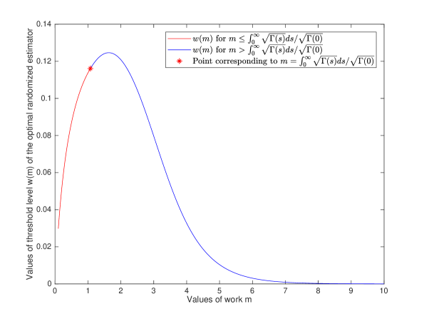
such that Uw(Imr)>Uw(Imf)subscript𝑈𝑤superscriptsubscript𝐼𝑚𝑟subscript𝑈𝑤superscriptsubscript𝐼𝑚𝑓U_{w}(I_{m}^{r})>U_{w}(I_{m}^{f}) for all 0<ww(m)0𝑤𝑤𝑚0<w\leq w(m). This threshold w(m)𝑤𝑚w(m) represents the maximum weight that a practitioner can put onto the variance such that the optimal randomized estimator is more favorable than the fixed truncation estimator. Similar to the proof in Proposition 1, it is straightforward to show that limm0w(m)=0subscript𝑚0𝑤𝑚0\lim_{m\to 0}w(m)=0. As discussed previously,

infQ(+):𝔼Q[N]=mVar(0Ng(Xs,s)Q(N>s)𝑑s)>Var(0g(Xs,s)𝑑s).subscriptinfimum:𝑄superscriptsuperscript𝔼𝑄delimited-[]𝑁𝑚Varsuperscriptsubscript0𝑁𝑔subscript𝑋𝑠𝑠𝑄𝑁𝑠differential-d𝑠Varsuperscriptsubscript0𝑔subscript𝑋𝑠𝑠differential-d𝑠\displaystyle\inf\limits_{Q\in\mathcal{M}(\mathbb{R}^{+}):\mathbb{E}^{Q}[N]=m}\mbox{Var}\left(\int_{0}^{N}\frac{g(X_{s},s)}{Q(N>s)}ds\right)>\mbox{Var}\left(\int_{0}^{\infty}g(X_{s},s)ds\right).

In the case where 0mg(Xs,s)𝑑ssuperscriptsubscript0𝑚𝑔subscript𝑋𝑠𝑠differential-d𝑠\int_{0}^{m}g(X_{s},s)ds and mg(Xs,s)𝑑ssuperscriptsubscript𝑚𝑔subscript𝑋𝑠𝑠differential-d𝑠\int_{m}^{\infty}g(X_{s},s)ds are positively correlated, then Var(0g(Xs,s)𝑑s)>Var(0mg(Xs,s)𝑑s)Varsuperscriptsubscript0𝑔subscript𝑋𝑠𝑠differential-d𝑠Varsuperscriptsubscript0𝑚𝑔subscript𝑋𝑠𝑠differential-d𝑠\mbox{Var}\left(\int_{0}^{\infty}g(X_{s},s)ds\right)>\mbox{Var}\left(\int_{0}^{m}g(X_{s},s)ds\right), which implies that w(m)𝑤𝑚w(m) is well defined and non-negative.

Proposition 2.

If {Xt}subscript𝑋𝑡\{X_{t}\} is an exponential Lévy process with characteristic exponent ϕitalic-ϕ\phi and f(x)=xβ𝑓𝑥superscript𝑥𝛽f(x)=x^{\beta}, then

w(m)={Δ1Δ2Δ4,0<m2|ϕ2(2β)|,Δ1Δ3Δ4,m>2|ϕ2(2β)|,𝑤𝑚casessubscriptΔ1subscriptΔ2subscriptΔ40𝑚2subscriptitalic-ϕ22𝛽otherwisesubscriptΔ1subscriptΔ3subscriptΔ4𝑚2subscriptitalic-ϕ22𝛽otherwise\displaystyle w(m)=\begin{cases}\frac{\Delta_{1}}{\Delta_{2}-\Delta_{4}},\quad 0<m\leq\frac{2}{|\phi_{2}(2\beta)|},\\ \frac{\Delta_{1}}{\Delta_{3}-\Delta_{4}},\quad m>\frac{2}{|\phi_{2}(2\beta)|},\end{cases}

where

Δ1:=e2|ϕ1(β)|m|ϕ1(β)|2,assignsubscriptΔ1superscript𝑒2subscriptitalic-ϕ1𝛽𝑚superscriptsubscriptitalic-ϕ1𝛽2\displaystyle\Delta_{1}:=\frac{e^{-2|\phi_{1}(\beta)|m}}{|\phi_{1}(\beta)|^{2}},
Δ2:=8m1|ϕ1(β)||ϕ2(2β)|21|ϕ1(β)|2,assignsubscriptΔ28𝑚1subscriptitalic-ϕ1𝛽superscriptsubscriptitalic-ϕ22𝛽21superscriptsubscriptitalic-ϕ1𝛽2\displaystyle\Delta_{2}:=\frac{8}{m}\frac{1}{|\phi_{1}(\beta)||\phi_{2}(2\beta)|^{2}}-\frac{1}{|\phi_{1}(\beta)|^{2}},
Δ3:=2+2em|ϕ2(2β)|+2|ϕ1(β)||ϕ2(2β)|1|ϕ1(β)|2,assignsubscriptΔ322superscript𝑒𝑚subscriptitalic-ϕ22𝛽2subscriptitalic-ϕ1𝛽subscriptitalic-ϕ22𝛽1superscriptsubscriptitalic-ϕ1𝛽2\displaystyle\Delta_{3}:=\frac{2+2e^{-m|\phi_{2}(2\beta)|+2}}{|\phi_{1}(\beta)||\phi_{2}(2\beta)|}-\frac{1}{|\phi_{1}(\beta)|^{2}},
Δ4:=2(1em|ϕ2(2β)|)|ϕ1(β)||ϕ2(2β)|+2em|ϕ2(2β)|2em|ϕ1(β)||ϕ1(β)|(|ϕ2(2β)||ϕ1(β)|)(1em|ϕ1(β)||ϕ1(β)|)2,assignsubscriptΔ421superscript𝑒𝑚subscriptitalic-ϕ22𝛽subscriptitalic-ϕ1𝛽subscriptitalic-ϕ22𝛽2superscript𝑒𝑚subscriptitalic-ϕ22𝛽2superscript𝑒𝑚subscriptitalic-ϕ1𝛽subscriptitalic-ϕ1𝛽subscriptitalic-ϕ22𝛽subscriptitalic-ϕ1𝛽superscript1superscript𝑒𝑚subscriptitalic-ϕ1𝛽subscriptitalic-ϕ1𝛽2\displaystyle\Delta_{4}:=\frac{2(1-e^{-m|\phi_{2}(2\beta)|})}{|\phi_{1}(\beta)||\phi_{2}(2\beta)|}+\frac{2e^{-m|\phi_{2}(2\beta)|}-2e^{-m|\phi_{1}(\beta)|}}{|\phi_{1}(\beta)|(|\phi_{2}(2\beta)|-|\phi_{1}(\beta)|)}-\left(\frac{1-e^{-m|\phi_{1}(\beta)|}}{|\phi_{1}(\beta)|}\right)^{2},

and ϕ1subscriptitalic-ϕ1\phi_{1} and ϕ2subscriptitalic-ϕ2\phi_{2} are given by (2.5).

Proof.

Recall that

𝔼[g(Xt,t)g(Xs,s)]=e(ts)ϕ1(β)+sϕ2(2β).𝔼delimited-[]𝑔subscript𝑋𝑡𝑡𝑔subscript𝑋𝑠𝑠superscript𝑒𝑡𝑠subscriptitalic-ϕ1𝛽𝑠subscriptitalic-ϕ22𝛽\mathbb{E}[g(X_{t},t)g(X_{s},s)]=e^{(t-s)\phi_{1}(\beta)+s\phi_{2}(2\beta)}.

and

Γ(s)=se(ts)ϕ1(β)+sϕ2(2β)𝑑t=1|ϕ1(β)|es|ϕ2(2β)|.Γ𝑠superscriptsubscript𝑠superscript𝑒𝑡𝑠subscriptitalic-ϕ1𝛽𝑠subscriptitalic-ϕ22𝛽differential-d𝑡1subscriptitalic-ϕ1𝛽superscript𝑒𝑠subscriptitalic-ϕ22𝛽\Gamma(s)=\int_{s}^{\infty}e^{(t-s)\phi_{1}(\beta)+s\phi_{2}(2\beta)}dt=\frac{1}{|\phi_{1}(\beta)|}e^{-s|\phi_{2}(2\beta)|}.

We have

(𝔼mg(Xs,s)𝑑s)2=(meϕ1(β)s𝑑s)2=Δ1,superscript𝔼superscriptsubscript𝑚𝑔subscript𝑋𝑠𝑠differential-d𝑠2superscriptsuperscriptsubscript𝑚superscript𝑒subscriptitalic-ϕ1𝛽𝑠differential-d𝑠2subscriptΔ1\left(\mathbb{E}\int_{m}^{\infty}g(X_{s},s)ds\right)^{2}=\left(\int_{m}^{\infty}e^{\phi_{1}(\beta)s}ds\right)^{2}=\Delta_{1},

and

(𝔼0g(Xs,s)𝑑s)2=1|ϕ1(β)|2.superscript𝔼superscriptsubscript0𝑔subscript𝑋𝑠𝑠differential-d𝑠21superscriptsubscriptitalic-ϕ1𝛽2\left(\mathbb{E}\int_{0}^{\infty}g(X_{s},s)ds\right)^{2}=\frac{1}{|\phi_{1}(\beta)|^{2}}.

In addition,

Var(0mg(Xs,s)𝑑s)Varsuperscriptsubscript0𝑚𝑔subscript𝑋𝑠𝑠differential-d𝑠\displaystyle\mbox{Var}\left(\int_{0}^{m}g(X_{s},s)ds\right) =𝔼[(0mg(Xs,s)𝑑s)2](𝔼0mg(Xs,s)𝑑s)2absent𝔼delimited-[]superscriptsuperscriptsubscript0𝑚𝑔subscript𝑋𝑠𝑠differential-d𝑠2superscript𝔼superscriptsubscript0𝑚𝑔subscript𝑋𝑠𝑠differential-d𝑠2\displaystyle=\mathbb{E}\left[\left(\int_{0}^{m}g(X_{s},s)ds\right)^{2}\right]-\left(\mathbb{E}\int_{0}^{m}g(X_{s},s)ds\right)^{2}
=2𝔼[0msmg(Xs,s)g(Xt,t)𝑑t𝑑s](𝔼0mg(Xs,s)𝑑s)2absent2𝔼delimited-[]superscriptsubscript0𝑚superscriptsubscript𝑠𝑚𝑔subscript𝑋𝑠𝑠𝑔subscript𝑋𝑡𝑡differential-d𝑡differential-d𝑠superscript𝔼superscriptsubscript0𝑚𝑔subscript𝑋𝑠𝑠differential-d𝑠2\displaystyle=2\mathbb{E}\left[\int_{0}^{m}\int_{s}^{m}g(X_{s},s)g(X_{t},t)dtds\right]-\left(\mathbb{E}\int_{0}^{m}g(X_{s},s)ds\right)^{2}
=20msme(ts)ϕ1(β)+sϕ2(2β)𝑑t𝑑s(0mesϕ1(β)𝑑s)2=Δ4.absent2superscriptsubscript0𝑚superscriptsubscript𝑠𝑚superscript𝑒𝑡𝑠subscriptitalic-ϕ1𝛽𝑠subscriptitalic-ϕ22𝛽differential-d𝑡differential-d𝑠superscriptsuperscriptsubscript0𝑚superscript𝑒𝑠subscriptitalic-ϕ1𝛽differential-d𝑠2subscriptΔ4\displaystyle=2\int_{0}^{m}\int_{s}^{m}e^{(t-s)\phi_{1}(\beta)+s\phi_{2}(2\beta)}dtds-\left(\int_{0}^{m}e^{s\phi_{1}(\beta)}ds\right)^{2}=\Delta_{4}.

For the optimal randomized estimator, from the result in Corollary 2, we have two cases. If m>2/|ϕ2(2β)|𝑚2subscriptitalic-ϕ22𝛽m>2/|\phi_{2}(2\beta)|, then the optimal Qsuperscript𝑄Q^{\ast} is given by

Q(N>s):={1for 0sm2|ϕ2(2β)|,em2|ϕ2(2β)|1s2|ϕ2(2β)|for s>m2|ϕ2(2β)|,assignsuperscript𝑄𝑁𝑠cases1for 0sm2|ϕ2(2β)|superscript𝑒𝑚2subscriptitalic-ϕ22𝛽1𝑠2subscriptitalic-ϕ22𝛽for s>m2|ϕ2(2β)|Q^{\ast}(N>s):=\begin{cases}1&\mbox{for $0\leq s\leq m-\frac{2}{|\phi_{2}(2\beta)|}$},\\ e^{\frac{m}{2}|\phi_{2}(2\beta)|-1-\frac{s}{2}|\phi_{2}(2\beta)|}&\mbox{for $s>m-\frac{2}{|\phi_{2}(2\beta)|}$},\end{cases}

and

Var(0Ng(Xs,s)Q(N>s)𝑑s)Varsuperscriptsubscript0𝑁𝑔subscript𝑋𝑠𝑠𝑄𝑁𝑠differential-d𝑠\displaystyle\mbox{Var}\left(\int_{0}^{N}\frac{g(X_{s},s)}{Q(N>s)}ds\right) =20Γ(s)Q(N>s)𝑑s(𝔼0g(Xs,s)𝑑s)2absent2superscriptsubscript0Γ𝑠superscript𝑄𝑁𝑠differential-d𝑠superscript𝔼superscriptsubscript0𝑔subscript𝑋𝑠𝑠differential-d𝑠2\displaystyle=2\int_{0}^{\infty}\frac{\Gamma(s)}{Q^{\ast}(N>s)}ds-\left(\mathbb{E}\int_{0}^{\infty}g(X_{s},s)ds\right)^{2}
=20m2|ϕ2(2β)|Γ(s)Q(N>s)𝑑s+2m2|ϕ2(2β)|Γ(s)Q(N>s)𝑑s1|ϕ1(β)|2absent2superscriptsubscript0𝑚2subscriptitalic-ϕ22𝛽Γ𝑠superscript𝑄𝑁𝑠differential-d𝑠2superscriptsubscript𝑚2subscriptitalic-ϕ22𝛽Γ𝑠superscript𝑄𝑁𝑠differential-d𝑠1superscriptsubscriptitalic-ϕ1𝛽2\displaystyle=2\int_{0}^{m-\frac{2}{|\phi_{2}(2\beta)|}}\frac{\Gamma(s)}{Q^{\ast}(N>s)}ds+2\int_{m-\frac{2}{|\phi_{2}(2\beta)|}}^{\infty}\frac{\Gamma(s)}{Q^{\ast}(N>s)}ds-\frac{1}{|\phi_{1}(\beta)|^{2}}
=20m2|ϕ2(2β)|Γ(s)𝑑s+2m2|ϕ2(2β)|Γ(s)Q(N>s)𝑑s1|ϕ1(β)|2absent2superscriptsubscript0𝑚2subscriptitalic-ϕ22𝛽Γ𝑠differential-d𝑠2superscriptsubscript𝑚2subscriptitalic-ϕ22𝛽Γ𝑠superscript𝑄𝑁𝑠differential-d𝑠1superscriptsubscriptitalic-ϕ1𝛽2\displaystyle=2\int_{0}^{m-\frac{2}{|\phi_{2}(2\beta)|}}\Gamma(s)ds+2\int_{m-\frac{2}{|\phi_{2}(2\beta)|}}^{\infty}\frac{\Gamma(s)}{Q^{\ast}(N>s)}ds-\frac{1}{|\phi_{1}(\beta)|^{2}}
=2(1e|ϕ2(2β)|m+2)|ϕ1(β)||ϕ2(2β)|+4e|ϕ2(2β)|m+2|ϕ1(β)||ϕ2(2β)|1|ϕ1(β)|2absent21superscript𝑒subscriptitalic-ϕ22𝛽𝑚2subscriptitalic-ϕ1𝛽subscriptitalic-ϕ22𝛽4superscript𝑒subscriptitalic-ϕ22𝛽𝑚2subscriptitalic-ϕ1𝛽subscriptitalic-ϕ22𝛽1superscriptsubscriptitalic-ϕ1𝛽2\displaystyle=\frac{2\left(1-e^{-|\phi_{2}(2\beta)|m+2}\right)}{|\phi_{1}(\beta)||\phi_{2}(2\beta)|}+\frac{4e^{-|\phi_{2}(2\beta)|m+2}}{|\phi_{1}(\beta)||\phi_{2}(2\beta)|}-\frac{1}{|\phi_{1}(\beta)|^{2}}
=2+2em|ϕ2(2β)|+2|ϕ1(β)||ϕ2(2β)|1|ϕ1(β)|2.absent22superscript𝑒𝑚subscriptitalic-ϕ22𝛽2subscriptitalic-ϕ1𝛽subscriptitalic-ϕ22𝛽1superscriptsubscriptitalic-ϕ1𝛽2\displaystyle=\frac{2+2e^{-m|\phi_{2}(2\beta)|+2}}{|\phi_{1}(\beta)||\phi_{2}(2\beta)|}-\frac{1}{|\phi_{1}(\beta)|^{2}}.

If m2/|ϕ2(2β)|𝑚2subscriptitalic-ϕ22𝛽m\leq 2/|\phi_{2}(2\beta)|, then the optimal Qsuperscript𝑄Q^{\ast} is given by

Q(N>s)=m2|ϕ2(2β)|es2|ϕ2(2β)|,superscript𝑄𝑁𝑠𝑚2subscriptitalic-ϕ22𝛽superscript𝑒𝑠2subscriptitalic-ϕ22𝛽Q^{\ast}(N>s)=\frac{m}{2}|\phi_{2}(2\beta)|e^{-\frac{s}{2}|\phi_{2}(2\beta)|},

and

Var(0Ng(Xs,s)Q(N>s)𝑑s)Varsuperscriptsubscript0𝑁𝑔subscript𝑋𝑠𝑠𝑄𝑁𝑠differential-d𝑠\displaystyle\mbox{Var}\left(\int_{0}^{N}\frac{g(X_{s},s)}{Q(N>s)}ds\right) =20Γ(s)Q(N>s)𝑑s(𝔼0g(Xs,s)𝑑s)2absent2superscriptsubscript0Γ𝑠superscript𝑄𝑁𝑠differential-d𝑠superscript𝔼superscriptsubscript0𝑔subscript𝑋𝑠𝑠differential-d𝑠2\displaystyle=2\int_{0}^{\infty}\frac{\Gamma(s)}{Q^{\ast}(N>s)}ds-\left(\mathbb{E}\int_{0}^{\infty}g(X_{s},s)ds\right)^{2}
=20Γ(s)Q(N>s)𝑑s1|ϕ1(β)|2=Δ2.absent2superscriptsubscript0Γ𝑠superscript𝑄𝑁𝑠differential-d𝑠1superscriptsubscriptitalic-ϕ1𝛽2subscriptΔ2\displaystyle=2\int_{0}^{\infty}\frac{\Gamma(s)}{Q^{\ast}(N>s)}ds-\frac{1}{|\phi_{1}(\beta)|^{2}}=\Delta_{2}~{}.

Then, it is straightforward to prove the conclusion. ∎

Next we offer an explicit expression for w(m)𝑤𝑚w(m) for the Cox-Ingersoll-Ross (CIR) process, which is an affine stochastic process not belonging to the class of exponential Lévy processes. The CIR process is governed by the following SDE:

dXt𝑑subscript𝑋𝑡\displaystyle dX_{t} =κ(θXt)dt+σXtdWt,absent𝜅𝜃subscript𝑋𝑡𝑑𝑡𝜎subscript𝑋𝑡𝑑subscript𝑊𝑡\displaystyle=\kappa(\theta-X_{t})dt+\sigma\sqrt{X_{t}}dW_{t},

where Wtsubscript𝑊𝑡W_{t} is a standard Brownian motion. The CIR process is mean reverting to θ𝜃\theta, and κ𝜅\kappa governs the speed of the mean reversion. According to the calculation in the appendix, we have

Γ(s)Γ𝑠\displaystyle\Gamma(s) =Ae2cs+Be(κ+2c)s+Ce2(κ+c)s,absent𝐴superscript𝑒2𝑐𝑠𝐵superscript𝑒𝜅2𝑐𝑠𝐶superscript𝑒2𝜅𝑐𝑠\displaystyle=Ae^{-2cs}+Be^{-(\kappa+2c)s}+Ce^{-2(\kappa+c)s},

where

A𝐴\displaystyle A :=θ2c+θσ22κ(κ+c),assignabsentsuperscript𝜃2𝑐𝜃superscript𝜎22𝜅𝜅𝑐\displaystyle:=\frac{\theta^{2}}{c}+\frac{\theta\sigma^{2}}{2\kappa(\kappa+c)},
B𝐵\displaystyle B :=1κ+c(X0θ)(θ+σ2κ)+θ(X0θ)c,assignabsent1𝜅𝑐subscript𝑋0𝜃𝜃superscript𝜎2𝜅𝜃subscript𝑋0𝜃𝑐\displaystyle:=\frac{1}{\kappa+c}(X_{0}-\theta)\left(\theta+\frac{\sigma^{2}}{\kappa}\right)+\frac{\theta(X_{0}-\theta)}{c},
C𝐶\displaystyle C :=1κ+c((θX0)2+σ22κ(θ2X0)).assignabsent1𝜅𝑐superscript𝜃subscript𝑋02superscript𝜎22𝜅𝜃2subscript𝑋0\displaystyle:=\frac{1}{\kappa+c}\left((\theta-X_{0})^{2}+\frac{\sigma^{2}}{2\kappa}(\theta-2X_{0})\right).
Proposition 3.

For the CIR process, we have

w(m)={(θcecm+X0θc+κe(c+κ)m)22m(0Γ(u)𝑑u)2α2Δ2, if 0<m0Γ(u)𝑑uΓ(0);(θcecm+X0θc+κe(c+κ)m)2Δ1Δ2, if m>0Γ(u)𝑑uΓ(0),𝑤𝑚casessuperscript𝜃𝑐superscript𝑒𝑐𝑚subscript𝑋0𝜃𝑐𝜅superscript𝑒𝑐𝜅𝑚22𝑚superscriptsuperscriptsubscript0Γ𝑢differential-d𝑢2superscript𝛼2subscriptsuperscriptΔ2 if 0𝑚superscriptsubscript0Γ𝑢differential-d𝑢Γ0otherwisesuperscript𝜃𝑐superscript𝑒𝑐𝑚subscript𝑋0𝜃𝑐𝜅superscript𝑒𝑐𝜅𝑚2subscriptsuperscriptΔ1subscriptsuperscriptΔ2 if 𝑚superscriptsubscript0Γ𝑢differential-d𝑢Γ0otherwise\displaystyle w(m)=\begin{cases}\frac{\left(\frac{\theta}{c}e^{-cm}+\frac{X_{0}-\theta}{c+\kappa}e^{-(c+\kappa)m}\right)^{2}}{\frac{2}{m}\left(\int_{0}^{\infty}\sqrt{\Gamma(u)}du\right)^{2}-\alpha^{2}-\Delta^{\prime}_{2}},\text{ if }0<m\leq\frac{\int_{0}^{\infty}\sqrt{\Gamma(u)}du}{\sqrt{\Gamma(0)}};\\ \frac{\left(\frac{\theta}{c}e^{-cm}+\frac{X_{0}-\theta}{c+\kappa}e^{-(c+\kappa)m}\right)^{2}}{\Delta^{\prime}_{1}-\Delta^{\prime}_{2}},\text{ if }m>\frac{\int_{0}^{\infty}\sqrt{\Gamma(u)}du}{\sqrt{\Gamma(0)}},\end{cases}

where

Δ1subscriptsuperscriptΔ1\displaystyle\Delta^{\prime}_{1} :=2(A1e2cs2c+B1e(κ+2c)sκ+2c+C1e2(κ+c)s2(κ+c))assignabsent2𝐴1superscript𝑒2𝑐superscript𝑠2𝑐𝐵1superscript𝑒𝜅2𝑐superscript𝑠𝜅2𝑐𝐶1superscript𝑒2𝜅𝑐superscript𝑠2𝜅𝑐\displaystyle:=2\left(A\frac{1-e^{-2cs^{\ast}}}{2c}+B\frac{1-e^{-(\kappa+2c)s^{\ast}}}{\kappa+2c}+C\frac{1-e^{-2(\kappa+c)s^{\ast}}}{2(\kappa+c)}\right)
+2(ms)(Ae2cs+Be(κ+2c)s+Ce2(κ+c)s)α2;2𝑚superscript𝑠𝐴superscript𝑒2𝑐superscript𝑠𝐵superscript𝑒𝜅2𝑐superscript𝑠𝐶superscript𝑒2𝜅𝑐superscript𝑠superscript𝛼2\displaystyle\quad\quad+2(m-s^{\ast})(Ae^{-2cs^{\ast}}+Be^{-(\kappa+2c)s^{\ast}}+Ce^{-2(\kappa+c)s^{\ast}})-\alpha^{2};
Δ2subscriptsuperscriptΔ2\displaystyle\Delta^{\prime}_{2} :=θ2c(1ecm)2+(X0θ)(θ+σ2κ)2c+κassignabsentsuperscript𝜃2𝑐superscript1superscript𝑒𝑐𝑚2subscript𝑋0𝜃𝜃superscript𝜎2𝜅2𝑐𝜅\displaystyle:=\frac{\theta^{2}}{c}(1-e^{-cm})^{2}+(X_{0}-\theta)\left(\theta+\frac{\sigma^{2}}{\kappa}\right)\frac{2}{c+\kappa}
×(1e(2c+κ)m2c+κe(c+κ)me(2c+κ)mc)absent1superscript𝑒2𝑐𝜅𝑚2𝑐𝜅superscript𝑒𝑐𝜅𝑚superscript𝑒2𝑐𝜅𝑚𝑐\displaystyle\quad\times\left(\frac{1-e^{-(2c+\kappa)m}}{2c+\kappa}-\frac{e^{-(c+\kappa)m}-e^{-(2c+\kappa)m}}{c}\right)
+2θ(X0θ)c(1e(2c+κ)m2c+κecme(2c+κ)mκ+c)2𝜃subscript𝑋0𝜃𝑐1superscript𝑒2𝑐𝜅𝑚2𝑐𝜅superscript𝑒𝑐𝑚superscript𝑒2𝑐𝜅𝑚𝜅𝑐\displaystyle\quad+\frac{2\theta(X_{0}-\theta)}{c}\left(\frac{1-e^{-(2c+\kappa)m}}{2c+\kappa}-\frac{e^{-cm}-e^{-(2c+\kappa)m}}{\kappa+c}\right)
+((θX0)2+σ22κ(θ2X0))(1e(κ+c)m)2κ+csuperscript𝜃subscript𝑋02superscript𝜎22𝜅𝜃2subscript𝑋0superscript1superscript𝑒𝜅𝑐𝑚2𝜅𝑐\displaystyle\quad+\left((\theta-X_{0})^{2}+\frac{\sigma^{2}}{2\kappa}(\theta-2X_{0})\right)\frac{(1-e^{-(\kappa+c)m})^{2}}{\kappa+c}
+θσ2κ(c+κ)(1e2cm2ce(c+κ)me2cmcκ)((X0θ)1e(c+κ)mc+κ+θ1ecmc)2,𝜃superscript𝜎2𝜅𝑐𝜅1superscript𝑒2𝑐𝑚2𝑐superscript𝑒𝑐𝜅𝑚superscript𝑒2𝑐𝑚𝑐𝜅superscriptsubscript𝑋0𝜃1superscript𝑒𝑐𝜅𝑚𝑐𝜅𝜃1superscript𝑒𝑐𝑚𝑐2\displaystyle\quad\quad+\frac{\theta\sigma^{2}}{\kappa(c+\kappa)}\left(\frac{1-e^{-2cm}}{2c}-\frac{e^{-(c+\kappa)m}-e^{-2cm}}{c-\kappa}\right)-\left((X_{0}-\theta)\frac{1-e^{-(c+\kappa)m}}{c+\kappa}+\theta\frac{1-e^{-cm}}{c}\right)^{2},

and Γ(0)=A+B+CΓ0𝐴𝐵𝐶\Gamma(0)=A+B+C. Here ssuperscript𝑠s^{\ast} is the unique positive solution to the following equation:

s+sΓ(s)𝑑sΓ(s)superscript𝑠superscriptsubscriptsuperscript𝑠Γ𝑠differential-d𝑠Γsuperscript𝑠\displaystyle s^{\ast}+\frac{\int_{s^{\ast}}^{\infty}{\sqrt{\Gamma(s)}ds}}{\sqrt{\Gamma(s^{\ast})}} =m.absent𝑚\displaystyle=m.

The proof of Proposition 3 can be found in the Appendix.

MSE Comparison for Exponential Lévy Process

Define

MSE1𝑀𝑆subscript𝐸1\displaystyle MSE_{1} :=Var(Im)+(𝔼[Im]α))2,\displaystyle:=Var(I_{m})+(\mathbb{E}[I_{m}]-\alpha))^{2},
MSE2𝑀𝑆subscript𝐸2\displaystyle MSE_{2} :=Var(IN).assignabsent𝑉𝑎𝑟subscript𝐼𝑁\displaystyle:=Var(I_{N}).

The randomized estimator is unbiased, so its MSE is just its variance.

Proposition 4.

For the exponential Lévy process, for all 0<m<0𝑚0<m<\infty,

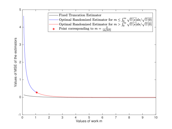
MSE1<MSE2.𝑀𝑆subscript𝐸1𝑀𝑆subscript𝐸2MSE_{1}<MSE_{2}.

The proof of Proposition 4 can be found in the Appendix.

4 Numerical Experiments

In this section, we present numerical experiments illustrating the main theoretical results. We choose the form of the discounted cost to be g(Xs,s)=ecsf(Xs)𝑔subscript𝑋𝑠𝑠superscript𝑒𝑐𝑠𝑓subscript𝑋𝑠g(X_{s},s)=e^{-cs}f(X_{s}) with c>0𝑐0c>0 denoting the continuous discount rate. Here f(Xs)𝑓subscript𝑋𝑠f(X_{s}) refers to the cost or reward at time s𝑠s, and we adopt the form f(x):=xβassign𝑓𝑥superscript𝑥𝛽f(x):=x^{\beta} motivated from the power utility function commonly used in decision theory and economics. As for the choice of the underlying stochastic process X𝑋X, we consider geometric Brownian motion (GBM) and the Cox-Ingersoll-Ross (CIR) process, which were also considered by Rhee and Glynn (2015) in their numerical experiments.

We first consider the example of discounted cost g(Xs,s)=ecsXsβ𝑔subscript𝑋𝑠𝑠superscript𝑒𝑐𝑠superscriptsubscript𝑋𝑠𝛽g(X_{s},s)=e^{-cs}X_{s}^{\beta} (c>0𝑐0c>0) with Xssubscript𝑋𝑠X_{s} being the geometric Brownian motion (GBM) model, which is a special case of the exponential Lévy process. The GBM model is governed by the following SDE:

dXt𝑑subscript𝑋𝑡\displaystyle dX_{t} =μXtdt+σXtdWt,X0=x0.formulae-sequenceabsent𝜇subscript𝑋𝑡𝑑𝑡𝜎subscript𝑋𝑡𝑑subscript𝑊𝑡subscript𝑋0subscript𝑥0\displaystyle=\mu X_{t}dt+\sigma X_{t}dW_{t},\quad X_{0}=x_{0}.

Then, we have ϕ(β)=(μσ22)β+σ22β2italic-ϕ𝛽𝜇superscript𝜎22𝛽superscript𝜎22superscript𝛽2\phi(\beta)=\left(\mu-\frac{\sigma^{2}}{2}\right)\beta+\frac{\sigma^{2}}{2}\beta^{2}. In addition, we can compute

Γ(s)=x02β|ϕ1(β)|es|ϕ2(2β)|,Γ𝑠superscriptsubscript𝑥02𝛽subscriptitalic-ϕ1𝛽superscript𝑒𝑠subscriptitalic-ϕ22𝛽\displaystyle\Gamma(s)=\frac{x_{0}^{2\beta}}{|\phi_{1}(\beta)|}e^{-s|\phi_{2}(2\beta)|},

and

α=0ecsx0β𝔼[esϕ(β)]𝑑s=x0βcϕ(β)=x0β|ϕ1(β)|.𝛼superscriptsubscript0superscript𝑒𝑐𝑠superscriptsubscript𝑥0𝛽𝔼delimited-[]superscript𝑒𝑠italic-ϕ𝛽differential-d𝑠superscriptsubscript𝑥0𝛽𝑐italic-ϕ𝛽superscriptsubscript𝑥0𝛽subscriptitalic-ϕ1𝛽\displaystyle\alpha=\int_{0}^{\infty}e^{-cs}x_{0}^{\beta}\mathbb{E}[e^{s\phi(\beta)}]ds=\frac{x_{0}^{\beta}}{c-\phi(\beta)}=\frac{x_{0}^{\beta}}{|\phi_{1}(\beta)|}.

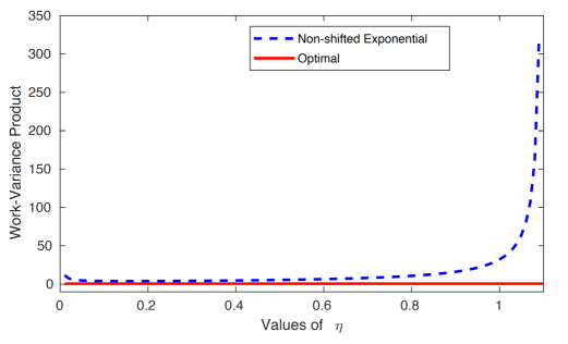
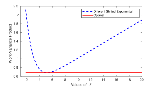
From Corollary 3, we know that the optimal randomization distribution is a shifted exponential distribution. The survival function of the shifted exponential distribution family is given by

Q(N>s)={1for sδ,eη(sδ)for s>δ.𝑄𝑁𝑠cases1for sδsuperscript𝑒𝜂𝑠𝛿for s>δQ(N>s)=\begin{cases}1&\mbox{for $s\leq\delta$},\\ e^{-\eta(s-\delta)}&\mbox{for $s>\delta$}.\end{cases}

The variance-work product of the shifted exponential distribution family can be expressed as a function of δ𝛿\delta and η𝜂\eta:

p(δ,η)𝑝𝛿𝜂\displaystyle p(\delta,\eta) :=Var(0g(Xs,s)1{N>s}Q(N>s)𝑑s)𝔼Q[N]assignabsentVarsuperscriptsubscript0𝑔subscript𝑋𝑠𝑠subscript1𝑁𝑠𝑄𝑁𝑠differential-d𝑠superscript𝔼𝑄delimited-[]𝑁\displaystyle:=\mbox{Var}\left(\int_{0}^{\infty}g(X_{s},s)\frac{1_{\{N>s\}}}{Q(N>s)}ds\right)\cdot\mathbb{E}^{Q}[N]
=(20Γ(s)Q(N>s)𝑑sα2)0Q(N>s)𝑑sabsent2superscriptsubscript0Γ𝑠𝑄𝑁𝑠differential-d𝑠superscript𝛼2superscriptsubscript0𝑄𝑁𝑠differential-d𝑠\displaystyle=\left(2\int_{0}^{\infty}\frac{\Gamma(s)}{Q(N>s)}ds-\alpha^{2}\right)\cdot\int_{0}^{\infty}Q(N>s)ds
=(2x0β1eδ|ϕ2(2β)||ϕ1(β)||ϕ2(2β)|+2x0βeδ|ϕ2(2β)||ϕ1(β)|(|ϕ2(2β)|η)α2)(δ+1η).absent2superscriptsubscript𝑥0𝛽1superscript𝑒𝛿subscriptitalic-ϕ22𝛽subscriptitalic-ϕ1𝛽subscriptitalic-ϕ22𝛽2superscriptsubscript𝑥0𝛽superscript𝑒𝛿subscriptitalic-ϕ22𝛽subscriptitalic-ϕ1𝛽subscriptitalic-ϕ22𝛽𝜂superscript𝛼2𝛿1𝜂\displaystyle=\left(2x_{0}^{\beta}\frac{1-e^{-\delta|\phi_{2}(2\beta)|}}{|\phi_{1}(\beta)||\phi_{2}(2\beta)|}+2x_{0}^{\beta}\frac{e^{-\delta|\phi_{2}(2\beta)|}}{|\phi_{1}(\beta)|(|\phi_{2}(2\beta)|-\eta)}-\alpha^{2}\right)\cdot\left(\delta+\frac{1}{\eta}\right).

Let η:=|ϕ2(2β)|/2assignsuperscript𝜂subscriptitalic-ϕ22𝛽2\eta^{*}:=|\phi_{2}(2\beta)|/2, which is the rate in the optimal randomization distribution. We set the parameters by x0=1subscript𝑥01x_{0}=1, μ=0.1𝜇0.1\mu=0.1, σ=0.35𝜎0.35\sigma=0.35, c=0.6𝑐0.6c=0.6, β=0.5𝛽0.5\beta=0.5. In this case, α=1.7689𝛼1.7689\alpha=1.7689, η=0.55superscript𝜂0.55\eta^{*}=0.55, s=4.7971superscript𝑠absent4.7971s^{\ast\ast}=4.7971, and the minimum work-variance product value is p(s,η)=0.68358𝑝superscript𝑠absentsuperscript𝜂0.68358p(s^{\ast\ast},\eta^{*})=0.68358.

Refer to caption
Figure 1: Comparison of non-shifted exponential to optimal distribution by varying η𝜂\eta

In Figure 1, the red line is the minimum work-variance product, and the blue line is the work-variance product function of a non-shifted exponential distribution, i.e., p(0,η)𝑝0𝜂p(0,\eta) with η[0.01,|ϕ2(2β)|]𝜂0.01subscriptitalic-ϕ22𝛽\eta\in[0.01,|\phi_{2}(2\beta)|]. We can see the variance-work product of the non-shifted exponential distribution family is strictly larger than the minimum work-variance product, which is consistent with the Theorem 3 result that the support of the optimal randomized distribution is always shifted away from zero. The work-variance product increases tremendously when η𝜂\eta grows larger than 0.60.60.6. A large η𝜂\eta would lead to a light tail for the survival function, which causes a large variance.
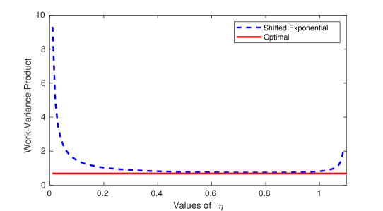
Refer to caption
Refer to caption
Figure 2: Comparison of shifted exponential to the optimal distribution by varying η𝜂\eta and δ𝛿\delta

In Figure 2, the blue line in the top graph plots the work-variance product function p(s,η)𝑝superscript𝑠𝜂p(s^{*},\eta) with η[0.01,|ϕ2(2β)|]𝜂0.01subscriptitalic-ϕ22𝛽\eta\in[0.01,|\phi_{2}(2\beta)|], while the blue line in the bottom graph is the work-variance product function p(δ,η)𝑝𝛿superscript𝜂p(\delta,\eta^{*}) with δ[2/|ϕ2(2β)|,20]𝛿2subscriptitalic-ϕ22𝛽20\delta\in[2/|\phi_{2}(2\beta)|,20]. We can see the two work-variance product functions deviate from the optimal value p(s,η)𝑝superscript𝑠superscript𝜂p(s^{*},\eta^{*}) except at the optimal point. The right panel in Figure 2 also substantiates the uniqueness of ssuperscript𝑠s^{*} in Theorem 3.

Then, we plot the threshold level w(m)𝑤𝑚w(m) given by Proposition 2 for this example. From Figure 3, we can see that even the optimal weight for all computational budget m𝑚m, which is the level of threshold w(m)𝑤𝑚w(m), is less than 0.130.130.13. This indicates that the advantage of the optimal randomized estimator over the fixed truncation estimator can only be justified under the scenario where the bias is the paramount concern.
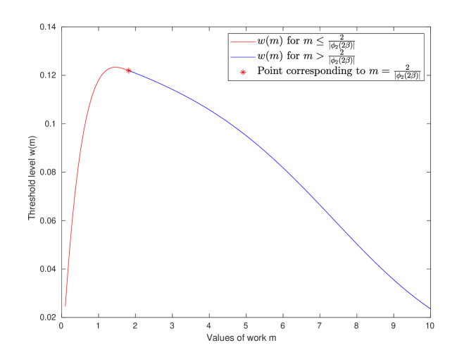
Refer to caption
Figure 3: MSE comparison between the fixed truncation estimator and the optimal randomized estimator

For w=1𝑤1w=1 in Uw(Im)subscript𝑈𝑤subscript𝐼𝑚U_{w}(I_{m}), this utility corresponds to the mean squared error (MSE), which is a widely used metric for the efficiency of an estimator. Figure 3 implies that the MSE of the optimal randomized estimator is always larger than the MSE of the fixed truncation estimator. Moreover, we prove in the Appendix that this conclusion holds for all exponential Lévy processes. The numerical results for the CIR process can be found in the appendix, which are similar to those for the exponential Lévy process.

5 Conclusion

In this paper, we propose a randomized unbiased estimator for simulating an expected cumulative cost/reward. We derive an explicit form for the optimal distribution of an unbiased randomized estimator balancing the trade-off between variance and computational cost. The optimal distributions are in a shifted distribution class. To the best of the authors’ knowledge, this is the first work resulting in explicit forms for the optimal randomization distribution. For a discounted continuous cumulative cost contingent on an exponential Lévy process, the optimal randomization distributions are shifted exponential distributions. The explicit structure of the distribution function of the optimal random truncation level is particularly useful for “post-estimation” analysis, and allows us to carry out a full diagnosis of the bias-variance tradeoff. Moreover, we justify the advantage of the optimal randomized estimator via a utility function taking both bias and variance into consideration. Our results are limited to simulating expected cumulative cost/reward. Future research lies in deriving the optimal randomized distribution and threshold level in the utility function for more general RUMC problems. Optimal control theory offers a new perspective to address such RUMC problems.

Acknowledgments.

We are grateful to the editor and two anonymous referees for their careful reading of the paper and very helpful suggestions. This work was supported in part by the National Science Foundation (NSF) under Grants CMMI-1362303, CMMI-1434419, and DMS-1613164, by the National Science Foundation of China (NSFC) under Grants 71901003, 71720107003, 91846301, 71790615, 71690232, and by the Air Force of Scientific Research (AFOSR) under Grant FA9550-15-10050.

References

  • Alexopoulos et al. (2016) Alexopoulos, C., Goldsman, D., Tang, P., Wilson, J.R., 2016. SPSTS: A sequential procedure for estimating the steady-state mean using standardized time series. IIE Transactions 48, 864–880.
  • Blanchet et al. (2015) Blanchet, J.H., Chen, N., Glynn, P.W., 2015. Unbiased Monte Carlo computation of smooth functions of expectations via taylor expansions, in: Proceedings of the Winter Simulation Conference, IEEE. pp. 360–367.
  • Blanchet and Sigman (2011) Blanchet, J.H., Sigman, K., 2011. On exact sampling of stochastic perpetuities. Journal of Applied Probability 48, 165–182.
  • Bryson and Ho (1975) Bryson, A.E., Ho, Y.C., 1975. Applied Optimal Control: Optimization, Estimation and Control. CRC Press.
  • Cui et al. (2019) Cui, Z., Lee, C., Zhu, L., Zhu, Y., 2019. On the optimal design of the randomized unbiased Monte Carlo estimators. Available at SSRN 3362534 .
  • Fox and Glynn (1989) Fox, B.L., Glynn, P.W., 1989. Simulating discounted costs. Management Science 35, 1297–1315.
  • Fu et al. (2017) Fu, M.C., Li, B., Li, G., Wu, R., 2017. Option pricing for a jump-diffusion model with general discrete jump-size distributions. Management Science 63, 3961–3977.
  • Giles (2008) Giles, M., 2008. Multilevel Monte Carlo path simulation. Operations Research 56, 607–617.
  • Giles (2015) Giles, M., 2015. Multilevel Monte Carlo methods. Acta Numerica 24, 259–328.
  • Glasserman and Staum (2003) Glasserman, P., Staum, J., 2003. Resource allocation among simulation time steps. Operations Research 51, 908–921.
  • Glynn (1983) Glynn, P.W., 1983. Randomized Estimators for Time Integrals. Technical Report. Mathematics Research Center, University of Wisconsin, Madison.
  • Glynn and Rhee (2014) Glynn, P.W., Rhee, C.H., 2014. Exact estimation for Markov chain equilibrium expectations. Journal of Applied Probability 51, 377–389.
  • Glynn and Whitt (1992) Glynn, P.W., Whitt, W., 1992. The asymptotic efficiency of simulation estimators. Operations Research 40, 505–520.
  • Halkin (1974) Halkin, H., 1974. Necessary conditions for optimal control problems with infinite horizons. Econometrica , 267–272.
  • Jacob et al. (2015) Jacob, P.E., Thiery, A.H., et al., 2015. On nonnegative unbiased estimators. The Annals of Statistics 43, 769–784.
  • Kahale (2019) Kahale, N., 2019. Optimal unbiased estimators via convex hulls. arXiv preprint:1909.02876 .
  • Lyne et al. (2015) Lyne, A.M., Girolami, M., Atchade, Y., Strathmann, H., Simpson, D., et al., 2015. On Russian roulette estimates for Bayesian inference with doubly-intractable likelihoods. Statistical Science 30, 443–467.
  • McLeish (2011) McLeish, D., 2011. A general method for debiasing a Monte Carlo estimator. Monte Carlo Methods and Applications 17, 301–315.
  • Merton (1969) Merton, R., 1969. Lifetime portfolio selection under uncertainty: The continuous-time case. Review of Economics and Statistics , 247–257.
  • Rhee and Glynn (2015) Rhee, C.h., Glynn, P.W., 2015. Unbiased estimation with square root convergence for SDE models. Operations Research 63, 1026–1043.
  • Vihola (2018) Vihola, M., 2018. Unbiased estimators and multilevel Monte Carlo. Operations Research 66, 448–462.
  • Whitt (2002) Whitt, W., 2002. Stochastic-Process Limits: An Introduction to Stochastic-Process Limits and their Application to Queues. Springer Science & Business Media.
  • Zheng and Glynn (2017) Zheng, Z., Glynn, P.W., 2017. A CLT for infinitely stratified estimators, with applications to debiased MLMC. ESAIM: Proceedings and Surveys 59, 104–114.

Appendix

Optimal Randomization for Non-Monotone Γ(s)Γ𝑠\Gamma(s)

Let z(s):=Q(N>s)assign𝑧𝑠𝑄𝑁𝑠z(s):=Q(N>s). Then, finding the optimal distribution can be viewed as finding the state corresponding to the following optimal control problem:

supu(s)(,0]0(2Γ(s)z(s)+λz(s))dssubscriptsupremum𝑢𝑠0superscriptsubscript02Γ𝑠𝑧𝑠𝜆𝑧𝑠𝑑𝑠\displaystyle\sup_{u(s)\in(-\infty,0]}\int_{0}^{\infty}-\left(\frac{2\Gamma(s)}{z(s)}+\lambda z(s)\right)ds
s.t.formulae-sequence𝑠𝑡\displaystyle s.t.~{} z˙(s)=u(s),z(0)=1,limtz(t)=0.formulae-sequence˙𝑧𝑠𝑢𝑠formulae-sequence𝑧01subscript𝑡𝑧𝑡0\displaystyle\dot{z}(s)=u(s),\quad z(0)=1,\quad\lim_{t\to\infty}z(t)=0.

Notice that the constraint u(s)(,0]𝑢𝑠0u(s)\in(-\infty,0] makes sure the state z(s)𝑧𝑠z(s) is non-increasing. The maximum principle gives a necessary condition of the optimal control:

p˙(s)=2Γ(s)z2(s)+λ,˙𝑝𝑠2Γ𝑠superscript𝑧2𝑠𝜆\displaystyle\dot{p}(s)=-\frac{2\Gamma(s)}{z^{2}(s)}+\lambda,
u(s)=argmax<u0H(z(s),u(s),p(t),s),superscript𝑢𝑠subscript𝑢0𝐻𝑧𝑠𝑢𝑠𝑝𝑡𝑠\displaystyle u^{*}(s)=\arg\max_{-\infty<u\leq 0}H(z(s),u(s),p(t),s),

where

H(z(s),u(s),p(t),s):=(2Γ(s)z(s)+λz(s))+p(s)u.assign𝐻𝑧𝑠𝑢𝑠𝑝𝑡𝑠2Γ𝑠𝑧𝑠𝜆𝑧𝑠𝑝𝑠𝑢H(z(s),u(s),p(t),s):=-\left(\frac{2\Gamma(s)}{z(s)}+\lambda z(s)\right)+p(s)u.

The necessary and sufficient condition for the optimal control can be given by the following Hamilton-Jacobi-Bellman (HJB) partial differential equation:

V˙(z,s)+minu{zV(z,s)u+(2Γ(s)z+λz)}=0,˙𝑉𝑧𝑠subscript𝑢subscript𝑧𝑉𝑧𝑠𝑢2Γ𝑠𝑧𝜆𝑧0\displaystyle\dot{V}(z,s)+\min_{u}\left\{\nabla_{z}V(z,s)u+\left(\frac{2\Gamma(s)}{z}+\lambda z\right)\right\}=0,

subject to the terminal condition limtV(x,t)=0subscript𝑡𝑉𝑥𝑡0\lim_{t\to\infty}V(x,t)=0.

Proof of Proposition 4

Proof.

If m>2/|ϕ2(2β)|𝑚2subscriptitalic-ϕ22𝛽m>2/|\phi_{2}(2\beta)|, we have

MSE1MSE2subscriptMSE1subscriptMSE2\displaystyle\text{MSE}_{1}-\text{MSE}_{2} =2(1em|ϕ2(2β)|)|ϕ1(β)||ϕ2(2β)|+2em|ϕ2(2β)|2em|ϕ1(β)||ϕ1(β)|(|ϕ2(2β)||ϕ1(β)|)absent21superscript𝑒𝑚subscriptitalic-ϕ22𝛽subscriptitalic-ϕ1𝛽subscriptitalic-ϕ22𝛽2superscript𝑒𝑚subscriptitalic-ϕ22𝛽2superscript𝑒𝑚subscriptitalic-ϕ1𝛽subscriptitalic-ϕ1𝛽subscriptitalic-ϕ22𝛽subscriptitalic-ϕ1𝛽\displaystyle=\frac{2(1-e^{-m|\phi_{2}(2\beta)|})}{|\phi_{1}(\beta)||\phi_{2}(2\beta)|}+\frac{2e^{-m|\phi_{2}(2\beta)|}-2e^{-m|\phi_{1}(\beta)|}}{|\phi_{1}(\beta)|(|\phi_{2}(2\beta)|-|\phi_{1}(\beta)|)}
(1em|ϕ1(β)||ϕ1(β)|)2+e2|ϕ1(β)|m|ϕ1(β)|2+1|ϕ1(β)|22+2em|ϕ2(2β)|+2|ϕ1(β)||ϕ2(2β)|.superscript1superscript𝑒𝑚subscriptitalic-ϕ1𝛽subscriptitalic-ϕ1𝛽2superscript𝑒2subscriptitalic-ϕ1𝛽𝑚superscriptsubscriptitalic-ϕ1𝛽21superscriptsubscriptitalic-ϕ1𝛽222superscript𝑒𝑚subscriptitalic-ϕ22𝛽2subscriptitalic-ϕ1𝛽subscriptitalic-ϕ22𝛽\displaystyle\quad-\left(\frac{1-e^{-m|\phi_{1}(\beta)|}}{|\phi_{1}(\beta)|}\right)^{2}+\frac{e^{-2|\phi_{1}(\beta)|m}}{|\phi_{1}(\beta)|^{2}}+\frac{1}{|\phi_{1}(\beta)|^{2}}-\frac{2+2e^{-m|\phi_{2}(2\beta)|+2}}{|\phi_{1}(\beta)||\phi_{2}(2\beta)|}.

Note that we can expand the term

(1em|ϕ1(β)||ϕ1(β)|)2superscript1superscript𝑒𝑚subscriptitalic-ϕ1𝛽subscriptitalic-ϕ1𝛽2\displaystyle\left(\frac{1-e^{-m|\phi_{1}(\beta)|}}{|\phi_{1}(\beta)|}\right)^{2} =1|ϕ1(β)|22em|ϕ1(β)||ϕ1(β)|2+e2m|ϕ1(β)||ϕ1(β)|2.absent1superscriptsubscriptitalic-ϕ1𝛽22superscript𝑒𝑚subscriptitalic-ϕ1𝛽superscriptsubscriptitalic-ϕ1𝛽2superscript𝑒2𝑚subscriptitalic-ϕ1𝛽superscriptsubscriptitalic-ϕ1𝛽2\displaystyle=\frac{1}{|\phi_{1}(\beta)|^{2}}-\frac{2e^{-m|\phi_{1}(\beta)|}}{|\phi_{1}(\beta)|^{2}}+\frac{e^{-2m|\phi_{1}(\beta)|}}{|\phi_{1}(\beta)|^{2}}.

Plugging in this expression into the above, we can further simplify the above expression to

MSE1MSE2subscriptMSE1subscriptMSE2\displaystyle\text{MSE}_{1}-\text{MSE}_{2}
=2(1em|ϕ2(2β)|)|ϕ1(β)||ϕ2(2β)|+2em|ϕ2(2β)|2em|ϕ1(β)||ϕ1(β)|(|ϕ2(2β)||ϕ1(β)|)+2em|ϕ1(β)||ϕ1(β)|22+2em|ϕ2(2β)|+2|ϕ1(β)||ϕ2(2β)|absent21superscript𝑒𝑚subscriptitalic-ϕ22𝛽subscriptitalic-ϕ1𝛽subscriptitalic-ϕ22𝛽2superscript𝑒𝑚subscriptitalic-ϕ22𝛽2superscript𝑒𝑚subscriptitalic-ϕ1𝛽subscriptitalic-ϕ1𝛽subscriptitalic-ϕ22𝛽subscriptitalic-ϕ1𝛽2superscript𝑒𝑚subscriptitalic-ϕ1𝛽superscriptsubscriptitalic-ϕ1𝛽222superscript𝑒𝑚subscriptitalic-ϕ22𝛽2subscriptitalic-ϕ1𝛽subscriptitalic-ϕ22𝛽\displaystyle=\frac{2(1-e^{-m|\phi_{2}(2\beta)|})}{|\phi_{1}(\beta)||\phi_{2}(2\beta)|}+\frac{2e^{-m|\phi_{2}(2\beta)|}-2e^{-m|\phi_{1}(\beta)|}}{|\phi_{1}(\beta)|(|\phi_{2}(2\beta)|-|\phi_{1}(\beta)|)}+\frac{2e^{-m|\phi_{1}(\beta)|}}{|\phi_{1}(\beta)|^{2}}-\frac{2+2e^{-m|\phi_{2}(2\beta)|+2}}{|\phi_{1}(\beta)||\phi_{2}(2\beta)|}
=2|ϕ1(β)|(1em|ϕ2(2β)||ϕ2(2β)|+em|ϕ2(2β)|em|ϕ1(β)||ϕ2(2β)||ϕ1(β)|+em|ϕ1(β)||ϕ1(β)|1+em|ϕ2(2β)|+2|ϕ2(2β)|)absent2subscriptitalic-ϕ1𝛽1superscript𝑒𝑚subscriptitalic-ϕ22𝛽subscriptitalic-ϕ22𝛽superscript𝑒𝑚subscriptitalic-ϕ22𝛽superscript𝑒𝑚subscriptitalic-ϕ1𝛽subscriptitalic-ϕ22𝛽subscriptitalic-ϕ1𝛽superscript𝑒𝑚subscriptitalic-ϕ1𝛽subscriptitalic-ϕ1𝛽1superscript𝑒𝑚subscriptitalic-ϕ22𝛽2subscriptitalic-ϕ22𝛽\displaystyle=\frac{2}{|\phi_{1}(\beta)|}\left(\frac{1-e^{-m|\phi_{2}(2\beta)|}}{|\phi_{2}(2\beta)|}+\frac{e^{-m|\phi_{2}(2\beta)|}-e^{-m|\phi_{1}(\beta)|}}{|\phi_{2}(2\beta)|-|\phi_{1}(\beta)|}+\frac{e^{-m|\phi_{1}(\beta)|}}{|\phi_{1}(\beta)|}-\frac{1+e^{-m|\phi_{2}(2\beta)|+2}}{|\phi_{2}(2\beta)|}\right)
=2|ϕ1(β)|(em|ϕ2(2β)|em|ϕ2(2β)|+2|ϕ2(2β)|+em|ϕ2(2β)|em|ϕ1(β)||ϕ2(2β)||ϕ1(β)|+em|ϕ1(β)||ϕ1(β)|).absent2subscriptitalic-ϕ1𝛽superscript𝑒𝑚subscriptitalic-ϕ22𝛽superscript𝑒𝑚subscriptitalic-ϕ22𝛽2subscriptitalic-ϕ22𝛽superscript𝑒𝑚subscriptitalic-ϕ22𝛽superscript𝑒𝑚subscriptitalic-ϕ1𝛽subscriptitalic-ϕ22𝛽subscriptitalic-ϕ1𝛽superscript𝑒𝑚subscriptitalic-ϕ1𝛽subscriptitalic-ϕ1𝛽\displaystyle=\frac{2}{|\phi_{1}(\beta)|}\left(\frac{-e^{-m|\phi_{2}(2\beta)|}-e^{-m|\phi_{2}(2\beta)|+2}}{|\phi_{2}(2\beta)|}+\frac{e^{-m|\phi_{2}(2\beta)|}-e^{-m|\phi_{1}(\beta)|}}{|\phi_{2}(2\beta)|-|\phi_{1}(\beta)|}+\frac{e^{-m|\phi_{1}(\beta)|}}{|\phi_{1}(\beta)|}\right).

Then we group the above terms by those related to em|ϕ1(β)|superscript𝑒𝑚subscriptitalic-ϕ1𝛽e^{-m|\phi_{1}(\beta)|} and those related to em|ϕ2(2β)|superscript𝑒𝑚subscriptitalic-ϕ22𝛽e^{-m|\phi_{2}(2\beta)|}, and we have

MSE1MSE2subscriptMSE1subscriptMSE2\displaystyle\text{MSE}_{1}-\text{MSE}_{2} =2|ϕ1(β)|(em|ϕ2(2β)|(1e2|ϕ2(2β)|+1|ϕ2(2β)||ϕ1(β)|)\displaystyle=\frac{2}{|\phi_{1}(\beta)|}\left(e^{-m|\phi_{2}(2\beta)|}\left(\frac{-1-e^{2}}{|\phi_{2}(2\beta)|}+\frac{1}{|\phi_{2}(2\beta)|-|\phi_{1}(\beta)|}\right)\right.
+em|ϕ1(β)|(1|ϕ1(β)|1|ϕ2(2β)||ϕ1(β)|))\displaystyle\left.\quad\quad+e^{-m|\phi_{1}(\beta)|}\left(\frac{1}{|\phi_{1}(\beta)|}-\frac{1}{|\phi_{2}(2\beta)|-|\phi_{1}(\beta)|}\right)\right)

From the Lévy-Khintchine formula and Jensen’s inequality, it is easy to establish that |ϕ2(2β)|<2|ϕ1(β)|subscriptitalic-ϕ22𝛽2subscriptitalic-ϕ1𝛽|\phi_{2}(2\beta)|<2|\phi_{1}(\beta)| always holds. Thus we have

1+e2|ϕ2(2β)|>1|ϕ1(β)|,1superscript𝑒2subscriptitalic-ϕ22𝛽1subscriptitalic-ϕ1𝛽\displaystyle\frac{1+e^{2}}{|\phi_{2}(2\beta)|}>\frac{1}{|\phi_{1}(\beta)|},

or equivalently we have

1e2|ϕ2(2β)|<1|ϕ1(β)|.1superscript𝑒2subscriptitalic-ϕ22𝛽1subscriptitalic-ϕ1𝛽\displaystyle\frac{-1-e^{2}}{|\phi_{2}(2\beta)|}<-\frac{1}{|\phi_{1}(\beta)|}.

Using this fact, we have

MSE1MSE2subscriptMSE1subscriptMSE2\displaystyle\text{MSE}_{1}-\text{MSE}_{2} =2|ϕ1(β)|(em|ϕ2(2β)|(1e2|ϕ2(2β)|+1|ϕ2(2β)||ϕ1(β)|)\displaystyle=\frac{2}{|\phi_{1}(\beta)|}\left(e^{-m|\phi_{2}(2\beta)|}\left(\frac{-1-e^{2}}{|\phi_{2}(2\beta)|}+\frac{1}{|\phi_{2}(2\beta)|-|\phi_{1}(\beta)|}\right)\right.
+em|ϕ1(β)|(1|ϕ1(β)|1|ϕ2(2β)||ϕ1(β)|))\displaystyle\left.\quad\quad+e^{-m|\phi_{1}(\beta)|}\left(\frac{1}{|\phi_{1}(\beta)|}-\frac{1}{|\phi_{2}(2\beta)|-|\phi_{1}(\beta)|}\right)\right)
<2|ϕ1(β)|(em|ϕ2(2β)|(1|ϕ1(β)|+1|ϕ2(2β)||ϕ1(β)|)\displaystyle<\frac{2}{|\phi_{1}(\beta)|}\left(e^{-m|\phi_{2}(2\beta)|}\left(-\frac{1}{|\phi_{1}(\beta)|}+\frac{1}{|\phi_{2}(2\beta)|-|\phi_{1}(\beta)|}\right)\right.
+em|ϕ1(β)|(1|ϕ1(β)|1|ϕ2(2β)||ϕ1(β)|))\displaystyle\left.\quad\quad+e^{-m|\phi_{1}(\beta)|}\left(\frac{1}{|\phi_{1}(\beta)|}-\frac{1}{|\phi_{2}(2\beta)|-|\phi_{1}(\beta)|}\right)\right)
=2|ϕ1(β)|(1|ϕ1(β)|1|ϕ2(2β)||ϕ1(β)|)(em|ϕ1(β)|em|ϕ2(2β)|).absent2subscriptitalic-ϕ1𝛽1subscriptitalic-ϕ1𝛽1subscriptitalic-ϕ22𝛽subscriptitalic-ϕ1𝛽superscript𝑒𝑚subscriptitalic-ϕ1𝛽superscript𝑒𝑚subscriptitalic-ϕ22𝛽\displaystyle=\frac{2}{|\phi_{1}(\beta)|}\left(\frac{1}{|\phi_{1}(\beta)|}-\frac{1}{|\phi_{2}(2\beta)|-|\phi_{1}(\beta)|}\right)\cdot\left(e^{-m|\phi_{1}(\beta)|}-e^{-m|\phi_{2}(2\beta)|}\right). (5.1)

We further divide the discussion into two cases:

  1. If |ϕ2(2β)||ϕ1(β)|>0subscriptitalic-ϕ22𝛽subscriptitalic-ϕ1𝛽0|\phi_{2}(2\beta)|-|\phi_{1}(\beta)|>0, then clearly we have 1|ϕ1(β)|1|ϕ2(2β)||ϕ1(β)|<01subscriptitalic-ϕ1𝛽1subscriptitalic-ϕ22𝛽subscriptitalic-ϕ1𝛽0\frac{1}{|\phi_{1}(\beta)|}-\frac{1}{|\phi_{2}(2\beta)|-|\phi_{1}(\beta)|}<0, and em|ϕ1(β)|em|ϕ2(2β)|>0superscript𝑒𝑚subscriptitalic-ϕ1𝛽superscript𝑒𝑚subscriptitalic-ϕ22𝛽0e^{-m|\phi_{1}(\beta)|}-e^{-m|\phi_{2}(2\beta)|}>0, thus the right hand side of (5.1) is negative.

  2. If |ϕ2(2β)||ϕ1(β)|<0subscriptitalic-ϕ22𝛽subscriptitalic-ϕ1𝛽0|\phi_{2}(2\beta)|-|\phi_{1}(\beta)|<0, then clearly we have 1|ϕ1(β)|1|ϕ2(2β)||ϕ1(β)|>01subscriptitalic-ϕ1𝛽1subscriptitalic-ϕ22𝛽subscriptitalic-ϕ1𝛽0\frac{1}{|\phi_{1}(\beta)|}-\frac{1}{|\phi_{2}(2\beta)|-|\phi_{1}(\beta)|}>0, and em|ϕ1(β)|em|ϕ2(2β)|<0superscript𝑒𝑚subscriptitalic-ϕ1𝛽superscript𝑒𝑚subscriptitalic-ϕ22𝛽0e^{-m|\phi_{1}(\beta)|}-e^{-m|\phi_{2}(2\beta)|}<0, thus the right hand side of (5.1) is negative.

Above all, we have proved that we always have MSE1MSE2<0subscriptMSE1subscriptMSE20\text{MSE}_{1}-\text{MSE}_{2}<0.

If m2/|ϕ2(2β)|𝑚2subscriptitalic-ϕ22𝛽m\leq 2/|\phi_{2}(2\beta)|, we have

MSE1MSE2subscriptMSE1subscriptMSE2\displaystyle\text{MSE}_{1}-\text{MSE}_{2} =2(1em|ϕ2(2β)|)|ϕ1(β)||ϕ2(2β)|+2em|ϕ2(2β)|2em|ϕ1(β)||ϕ1(β)|(|ϕ2(2β)||ϕ1(β)|)absent21superscript𝑒𝑚subscriptitalic-ϕ22𝛽subscriptitalic-ϕ1𝛽subscriptitalic-ϕ22𝛽2superscript𝑒𝑚subscriptitalic-ϕ22𝛽2superscript𝑒𝑚subscriptitalic-ϕ1𝛽subscriptitalic-ϕ1𝛽subscriptitalic-ϕ22𝛽subscriptitalic-ϕ1𝛽\displaystyle=\frac{2(1-e^{-m|\phi_{2}(2\beta)|})}{|\phi_{1}(\beta)||\phi_{2}(2\beta)|}+\frac{2e^{-m|\phi_{2}(2\beta)|}-2e^{-m|\phi_{1}(\beta)|}}{|\phi_{1}(\beta)|(|\phi_{2}(2\beta)|-|\phi_{1}(\beta)|)}
(1em|ϕ1(β)||ϕ1(β)|)2+e2|ϕ1(β)|m|ϕ1(β)|2+1|ϕ1(β)|28m1|ϕ1(β)||ϕ2(2β)|2.superscript1superscript𝑒𝑚subscriptitalic-ϕ1𝛽subscriptitalic-ϕ1𝛽2superscript𝑒2subscriptitalic-ϕ1𝛽𝑚superscriptsubscriptitalic-ϕ1𝛽21superscriptsubscriptitalic-ϕ1𝛽28𝑚1subscriptitalic-ϕ1𝛽superscriptsubscriptitalic-ϕ22𝛽2\displaystyle\qquad-\left(\frac{1-e^{-m|\phi_{1}(\beta)|}}{|\phi_{1}(\beta)|}\right)^{2}+\frac{e^{-2|\phi_{1}(\beta)|m}}{|\phi_{1}(\beta)|^{2}}+\frac{1}{|\phi_{1}(\beta)|^{2}}-\frac{8}{m}\frac{1}{|\phi_{1}(\beta)||\phi_{2}(2\beta)|^{2}}.

Note that we can expand the term

(1em|ϕ1(β)||ϕ1(β)|)2superscript1superscript𝑒𝑚subscriptitalic-ϕ1𝛽subscriptitalic-ϕ1𝛽2\displaystyle\left(\frac{1-e^{-m|\phi_{1}(\beta)|}}{|\phi_{1}(\beta)|}\right)^{2} =1|ϕ1(β)|22em|ϕ1(β)||ϕ1(β)|2+e2m|ϕ1(β)||ϕ1(β)|2.absent1superscriptsubscriptitalic-ϕ1𝛽22superscript𝑒𝑚subscriptitalic-ϕ1𝛽superscriptsubscriptitalic-ϕ1𝛽2superscript𝑒2𝑚subscriptitalic-ϕ1𝛽superscriptsubscriptitalic-ϕ1𝛽2\displaystyle=\frac{1}{|\phi_{1}(\beta)|^{2}}-\frac{2e^{-m|\phi_{1}(\beta)|}}{|\phi_{1}(\beta)|^{2}}+\frac{e^{-2m|\phi_{1}(\beta)|}}{|\phi_{1}(\beta)|^{2}}.

Plugging in this expression into the above, we can further simplify the above expression to

MSE1MSE2subscriptMSE1subscriptMSE2\displaystyle\text{MSE}_{1}-\text{MSE}_{2} =2(1em|ϕ2(2β)|)|ϕ1(β)||ϕ2(2β)|+2em|ϕ2(2β)|2em|ϕ1(β)||ϕ1(β)|(|ϕ2(2β)||ϕ1(β)|)absent21superscript𝑒𝑚subscriptitalic-ϕ22𝛽subscriptitalic-ϕ1𝛽subscriptitalic-ϕ22𝛽2superscript𝑒𝑚subscriptitalic-ϕ22𝛽2superscript𝑒𝑚subscriptitalic-ϕ1𝛽subscriptitalic-ϕ1𝛽subscriptitalic-ϕ22𝛽subscriptitalic-ϕ1𝛽\displaystyle=\frac{2(1-e^{-m|\phi_{2}(2\beta)|})}{|\phi_{1}(\beta)||\phi_{2}(2\beta)|}+\frac{2e^{-m|\phi_{2}(2\beta)|}-2e^{-m|\phi_{1}(\beta)|}}{|\phi_{1}(\beta)|(|\phi_{2}(2\beta)|-|\phi_{1}(\beta)|)}
+2em|ϕ1(β)||ϕ1(β)|28m1|ϕ1(β)||ϕ2(2β)|22superscript𝑒𝑚subscriptitalic-ϕ1𝛽superscriptsubscriptitalic-ϕ1𝛽28𝑚1subscriptitalic-ϕ1𝛽superscriptsubscriptitalic-ϕ22𝛽2\displaystyle\quad+\frac{2e^{-m|\phi_{1}(\beta)|}}{|\phi_{1}(\beta)|^{2}}-\frac{8}{m}\frac{1}{|\phi_{1}(\beta)||\phi_{2}(2\beta)|^{2}}
=2|ϕ1(β)|(1em|ϕ2(2β)||ϕ2(2β)|+em|ϕ2(2β)|em|ϕ1(β)||ϕ2(2β)||ϕ1(β)|\displaystyle=\frac{2}{|\phi_{1}(\beta)|}\left(\frac{1-e^{-m|\phi_{2}(2\beta)|}}{|\phi_{2}(2\beta)|}+\frac{e^{-m|\phi_{2}(2\beta)|}-e^{-m|\phi_{1}(\beta)|}}{|\phi_{2}(2\beta)|-|\phi_{1}(\beta)|}\right.
+em|ϕ1(β)||ϕ1(β)|4m|ϕ2(2β)|2)\displaystyle\qquad\qquad\qquad\left.+\frac{e^{-m|\phi_{1}(\beta)|}}{|\phi_{1}(\beta)|}-\frac{4}{m|\phi_{2}(2\beta)|^{2}}\right)
<2|ϕ1(β)|(1em|ϕ2(2β)||ϕ2(2β)|+em|ϕ2(2β)|em|ϕ1(β)||ϕ2(2β)||ϕ1(β)|\displaystyle<\frac{2}{|\phi_{1}(\beta)|}\left(\frac{1-e^{-m|\phi_{2}(2\beta)|}}{|\phi_{2}(2\beta)|}+\frac{e^{-m|\phi_{2}(2\beta)|}-e^{-m|\phi_{1}(\beta)|}}{|\phi_{2}(2\beta)|-|\phi_{1}(\beta)|}\right.
+em|ϕ1(β)||ϕ1(β)|2|ϕ2(2β)|)\displaystyle\left.\qquad\qquad\qquad+\frac{e^{-m|\phi_{1}(\beta)|}}{|\phi_{1}(\beta)|}-\frac{2}{|\phi_{2}(2\beta)|}\right)
=2|ϕ1(β)|(1em|ϕ2(2β)||ϕ2(2β)|+em|ϕ2(2β)|em|ϕ1(β)||ϕ2(2β)||ϕ1(β)|+em|ϕ1(β)||ϕ1(β)|)absent2subscriptitalic-ϕ1𝛽1superscript𝑒𝑚subscriptitalic-ϕ22𝛽subscriptitalic-ϕ22𝛽superscript𝑒𝑚subscriptitalic-ϕ22𝛽superscript𝑒𝑚subscriptitalic-ϕ1𝛽subscriptitalic-ϕ22𝛽subscriptitalic-ϕ1𝛽superscript𝑒𝑚subscriptitalic-ϕ1𝛽subscriptitalic-ϕ1𝛽\displaystyle=\frac{2}{|\phi_{1}(\beta)|}\left(\frac{-1-e^{-m|\phi_{2}(2\beta)|}}{|\phi_{2}(2\beta)|}+\frac{e^{-m|\phi_{2}(2\beta)|}-e^{-m|\phi_{1}(\beta)|}}{|\phi_{2}(2\beta)|-|\phi_{1}(\beta)|}+\frac{e^{-m|\phi_{1}(\beta)|}}{|\phi_{1}(\beta)|}\right)
<2|ϕ1(β)|(2em|ϕ2(2β)||ϕ2(2β)|+em|ϕ2(2β)|em|ϕ1(β)||ϕ2(2β)||ϕ1(β)|+em|ϕ1(β)||ϕ1(β)|),absent2subscriptitalic-ϕ1𝛽2superscript𝑒𝑚subscriptitalic-ϕ22𝛽subscriptitalic-ϕ22𝛽superscript𝑒𝑚subscriptitalic-ϕ22𝛽superscript𝑒𝑚subscriptitalic-ϕ1𝛽subscriptitalic-ϕ22𝛽subscriptitalic-ϕ1𝛽superscript𝑒𝑚subscriptitalic-ϕ1𝛽subscriptitalic-ϕ1𝛽\displaystyle<\frac{2}{|\phi_{1}(\beta)|}\left(\frac{-2e^{-m|\phi_{2}(2\beta)|}}{|\phi_{2}(2\beta)|}+\frac{e^{-m|\phi_{2}(2\beta)|}-e^{-m|\phi_{1}(\beta)|}}{|\phi_{2}(2\beta)|-|\phi_{1}(\beta)|}+\frac{e^{-m|\phi_{1}(\beta)|}}{|\phi_{1}(\beta)|}\right),

where in the second last inequality, we have utilized the assumption that m|ϕ2(2β)|<2𝑚subscriptitalic-ϕ22𝛽2m|\phi_{2}(2\beta)|<2, and in the last inequality we have used the fact that em|ϕ2(2β)|<1superscript𝑒𝑚subscriptitalic-ϕ22𝛽1e^{-m|\phi_{2}(2\beta)|}<1.

Then we group the above terms by those related to em|ϕ1(β)|superscript𝑒𝑚subscriptitalic-ϕ1𝛽e^{-m|\phi_{1}(\beta)|} and those related to em|ϕ2(2β)|superscript𝑒𝑚subscriptitalic-ϕ22𝛽e^{-m|\phi_{2}(2\beta)|}:

MSE1MSE2subscriptMSE1subscriptMSE2\displaystyle\text{MSE}_{1}-\text{MSE}_{2} <2|ϕ1(β)|(em|ϕ2(2β)|(2|ϕ2(2β)|+1|ϕ2(2β)||ϕ1(β)|)\displaystyle<\frac{2}{|\phi_{1}(\beta)|}\left(e^{-m|\phi_{2}(2\beta)|}\left(\frac{-2}{|\phi_{2}(2\beta)|}+\frac{1}{|\phi_{2}(2\beta)|-|\phi_{1}(\beta)|}\right)\right.
+em|ϕ1(β)|(1|ϕ1(β)|1|ϕ2(2β)||ϕ1(β)|))\displaystyle\left.\quad\quad+e^{-m|\phi_{1}(\beta)|}\left(\frac{1}{|\phi_{1}(\beta)|}-\frac{1}{|\phi_{2}(2\beta)|-|\phi_{1}(\beta)|}\right)\right)

From the Lévy-Khintchine formula and the Jensen inequality, it is easy to establish that |ϕ2(2β)|<2|ϕ1(β)|subscriptitalic-ϕ22𝛽2subscriptitalic-ϕ1𝛽|\phi_{2}(2\beta)|<2|\phi_{1}(\beta)| always holds. Thus we have

2|ϕ2(2β)|<1|ϕ1(β)|.2subscriptitalic-ϕ22𝛽1subscriptitalic-ϕ1𝛽\displaystyle\frac{-2}{|\phi_{2}(2\beta)|}<-\frac{1}{|\phi_{1}(\beta)|}.

Thus we have

MSE1MSE2subscriptMSE1subscriptMSE2\displaystyle\text{MSE}_{1}-\text{MSE}_{2} <2|ϕ1(β)|(em|ϕ2(2β)|(2|ϕ2(2β)|+1|ϕ2(2β)||ϕ1(β)|)\displaystyle<\frac{2}{|\phi_{1}(\beta)|}\left(e^{-m|\phi_{2}(2\beta)|}\left(\frac{-2}{|\phi_{2}(2\beta)|}+\frac{1}{|\phi_{2}(2\beta)|-|\phi_{1}(\beta)|}\right)\right.
+em|ϕ1(β)|(1|ϕ1(β)|1|ϕ2(2β)||ϕ1(β)|))\displaystyle\left.\quad\quad+e^{-m|\phi_{1}(\beta)|}\left(\frac{1}{|\phi_{1}(\beta)|}-\frac{1}{|\phi_{2}(2\beta)|-|\phi_{1}(\beta)|}\right)\right)
<2|ϕ1(β)|(em|ϕ2(2β)|(1|ϕ1(β)|+1|ϕ2(2β)||ϕ1(β)|)\displaystyle<\frac{2}{|\phi_{1}(\beta)|}\left(e^{-m|\phi_{2}(2\beta)|}\left(-\frac{1}{|\phi_{1}(\beta)|}+\frac{1}{|\phi_{2}(2\beta)|-|\phi_{1}(\beta)|}\right)\right.
+em|ϕ1(β)|(1|ϕ1(β)|1|ϕ2(2β)||ϕ1(β)|))\displaystyle\left.\quad\quad+e^{-m|\phi_{1}(\beta)|}\left(\frac{1}{|\phi_{1}(\beta)|}-\frac{1}{|\phi_{2}(2\beta)|-|\phi_{1}(\beta)|}\right)\right)
=2|ϕ1(β)|(1|ϕ1(β)|1|ϕ2(2β)||ϕ1(β)|)(em|ϕ1(β)|em|ϕ2(2β)|).absent2subscriptitalic-ϕ1𝛽1subscriptitalic-ϕ1𝛽1subscriptitalic-ϕ22𝛽subscriptitalic-ϕ1𝛽superscript𝑒𝑚subscriptitalic-ϕ1𝛽superscript𝑒𝑚subscriptitalic-ϕ22𝛽\displaystyle=\frac{2}{|\phi_{1}(\beta)|}\left(\frac{1}{|\phi_{1}(\beta)|}-\frac{1}{|\phi_{2}(2\beta)|-|\phi_{1}(\beta)|}\right)\cdot\left(e^{-m|\phi_{1}(\beta)|}-e^{-m|\phi_{2}(2\beta)|}\right). (5.2)

Note that the right hand side of (5.2) is exactly the same as the right hand side of (5.1), thus following similar arguments, we can establish that MSE1MSE3<0𝑀𝑆subscript𝐸1𝑀𝑆subscript𝐸30MSE_{1}-MSE_{3}<0. This completes the proof. ∎

Derivations for the CIR process

We can compute that

α=0ecs𝔼[Xs]𝑑s𝛼superscriptsubscript0superscript𝑒𝑐𝑠𝔼delimited-[]subscript𝑋𝑠differential-d𝑠\displaystyle\alpha=\int_{0}^{\infty}e^{-cs}\mathbb{E}[X_{s}]ds =0ecs(X0eκs+θ(1eκs))𝑑s=θc+X0θκ+c.absentsuperscriptsubscript0superscript𝑒𝑐𝑠subscript𝑋0superscript𝑒𝜅𝑠𝜃1superscript𝑒𝜅𝑠differential-d𝑠𝜃𝑐subscript𝑋0𝜃𝜅𝑐\displaystyle=\int_{0}^{\infty}e^{-cs}\left(X_{0}e^{-\kappa s}+\theta(1-e^{-\kappa s})\right)ds=\frac{\theta}{c}+\frac{X_{0}-\theta}{\kappa+c}.

We have the following expression for its cross moment for s<t𝑠𝑡s<t

𝔼[XsXt]=𝔼delimited-[]subscript𝑋𝑠subscript𝑋𝑡absent\displaystyle\mathbb{E}[X_{s}X_{t}]= θ2+eκt(X0θ)(θ+σ2κ)+eκsθ(X0θ)superscript𝜃2superscript𝑒𝜅𝑡subscript𝑋0𝜃𝜃superscript𝜎2𝜅superscript𝑒𝜅𝑠𝜃subscript𝑋0𝜃\displaystyle\theta^{2}+e^{-\kappa t}(X_{0}-\theta)\left(\theta+\frac{\sigma^{2}}{\kappa}\right)+e^{-\kappa s}\theta(X_{0}-\theta)
+eκ(t+s)((θX0)2+σ22κ(θ2X0))+θσ22κeκ(ts).superscript𝑒𝜅𝑡𝑠superscript𝜃subscript𝑋02superscript𝜎22𝜅𝜃2subscript𝑋0𝜃superscript𝜎22𝜅superscript𝑒𝜅𝑡𝑠\displaystyle+e^{-\kappa(t+s)}\left((\theta-X_{0})^{2}+\frac{\sigma^{2}}{2\kappa}(\theta-2X_{0})\right)+\frac{\theta\sigma^{2}}{2\kappa}e^{-\kappa(t-s)}.

Define the process Yt:=ectXtassignsubscript𝑌𝑡superscript𝑒𝑐𝑡subscript𝑋𝑡Y_{t}:=e^{-ct}X_{t}, then we have

𝔼[YsYt]𝔼delimited-[]subscript𝑌𝑠subscript𝑌𝑡\displaystyle\mathbb{E}[Y_{s}Y_{t}] =ec(t+s)𝔼[XsXt]absentsuperscript𝑒𝑐𝑡𝑠𝔼delimited-[]subscript𝑋𝑠subscript𝑋𝑡\displaystyle=e^{-c(t+s)}\mathbb{E}[X_{s}X_{t}]
=θ2ec(t+s)+ecs(κ+c)t(X0θ)(θ+σ2κ)+e(κ+c)sctθ(X0θ)absentsuperscript𝜃2superscript𝑒𝑐𝑡𝑠superscript𝑒𝑐𝑠𝜅𝑐𝑡subscript𝑋0𝜃𝜃superscript𝜎2𝜅superscript𝑒𝜅𝑐𝑠𝑐𝑡𝜃subscript𝑋0𝜃\displaystyle=\theta^{2}e^{-c(t+s)}+e^{-cs-(\kappa+c)t}(X_{0}-\theta)\left(\theta+\frac{\sigma^{2}}{\kappa}\right)+e^{-(\kappa+c)s-ct}\theta(X_{0}-\theta)
+e(κ+c)(t+s)((θX0)2+σ22κ(θ2X0))+θσ22κe(c+κ)t(cκ)s.superscript𝑒𝜅𝑐𝑡𝑠superscript𝜃subscript𝑋02superscript𝜎22𝜅𝜃2subscript𝑋0𝜃superscript𝜎22𝜅superscript𝑒𝑐𝜅𝑡𝑐𝜅𝑠\displaystyle\quad+e^{-(\kappa+c)(t+s)}\left((\theta-X_{0})^{2}+\frac{\sigma^{2}}{2\kappa}(\theta-2X_{0})\right)+\frac{\theta\sigma^{2}}{2\kappa}e^{-(c+\kappa)t-(c-\kappa)s}.

For f(x)=x𝑓𝑥𝑥f(x)=x, we have

Γ(s)Γ𝑠\displaystyle\Gamma(s) =s𝔼[ecsf(Xs)ectf(Xt)]=s𝔼[YsYt]𝑑tabsentsuperscriptsubscript𝑠𝔼delimited-[]superscript𝑒𝑐𝑠𝑓subscript𝑋𝑠superscript𝑒𝑐𝑡𝑓subscript𝑋𝑡superscriptsubscript𝑠𝔼delimited-[]subscript𝑌𝑠subscript𝑌𝑡differential-d𝑡\displaystyle=\int_{s}^{\infty}\mathbb{E}[e^{-cs}f(X_{s})e^{-ct}f(X_{t})]=\int_{s}^{\infty}\mathbb{E}[Y_{s}Y_{t}]dt
=θ2ce2cs+e(κ+2c)sκ+c(X0θ)(θ+σ2κ)+e(κ+2c)scθ(X0θ)absentsuperscript𝜃2𝑐superscript𝑒2𝑐𝑠superscript𝑒𝜅2𝑐𝑠𝜅𝑐subscript𝑋0𝜃𝜃superscript𝜎2𝜅superscript𝑒𝜅2𝑐𝑠𝑐𝜃subscript𝑋0𝜃\displaystyle=\frac{\theta^{2}}{c}e^{-2cs}+\frac{e^{-(\kappa+2c)s}}{\kappa+c}(X_{0}-\theta)\left(\theta+\frac{\sigma^{2}}{\kappa}\right)+\frac{e^{-(\kappa+2c)s}}{c}\theta(X_{0}-\theta)
+e2(κ+c)sκ+c((θX0)2+σ22κ(θ2X0))+θσ22κe2csκ+c.superscript𝑒2𝜅𝑐𝑠𝜅𝑐superscript𝜃subscript𝑋02superscript𝜎22𝜅𝜃2subscript𝑋0𝜃superscript𝜎22𝜅superscript𝑒2𝑐𝑠𝜅𝑐\displaystyle+\frac{e^{-2(\kappa+c)s}}{\kappa+c}\left((\theta-X_{0})^{2}+\frac{\sigma^{2}}{2\kappa}(\theta-2X_{0})\right)+\frac{\theta\sigma^{2}}{2\kappa}\frac{e^{-2cs}}{\kappa+c}. (5.3)

Here we have to determine the sufficient conditions to be imposed onto the parameters in order to have the Assumption 1 to be satisfied. A sufficient condition is given by

θ(X0θ)𝜃subscript𝑋0𝜃\displaystyle\theta(X_{0}-\theta) >0,(θX0)2+σ22κ(θ2X0)>0,formulae-sequenceabsent0superscript𝜃subscript𝑋02superscript𝜎22𝜅𝜃2subscript𝑋00\displaystyle>0,\quad(\theta-X_{0})^{2}+\frac{\sigma^{2}}{2\kappa}(\theta-2X_{0})>0,

which is equivalent to requiring

X0subscript𝑋0\displaystyle X_{0} >θ+σ22κ+σ22κ(θ+σ22κ).absent𝜃superscript𝜎22𝜅superscript𝜎22𝜅𝜃superscript𝜎22𝜅\displaystyle>\theta+\frac{\sigma^{2}}{2\kappa}+\sqrt{\frac{\sigma^{2}}{2\kappa}\left(\theta+\frac{\sigma^{2}}{2\kappa}\right)}.

Then we calculate the ingredients for the determination of the optimal randomization distribution. For example, in the case of solving the optimization problem (2.2), from the result in Theorem 1, we have

Q(N>s)={10ss,2(Ae2cs+Be(κ+2c)s+Ce2(κ+c)s)λs>s,superscript𝑄𝑁𝑠cases10𝑠superscript𝑠2𝐴superscript𝑒2𝑐𝑠𝐵superscript𝑒𝜅2𝑐𝑠𝐶superscript𝑒2𝜅𝑐𝑠𝜆𝑠superscript𝑠Q^{\ast}(N>s)=\begin{cases}1&\mbox{$0\leq s\leq s^{\ast}$},\\ \sqrt{\frac{2(Ae^{-2cs}+Be^{-(\kappa+2c)s}+Ce^{-2(\kappa+c)s})}{\lambda}}&\mbox{$s>s^{\ast}$},\end{cases}

where s=inf{s[0,):Ae2cs+Be(κ+2c)s+Ce2(κ+c)sλ/2}superscript𝑠infimumconditional-set𝑠0𝐴superscript𝑒2𝑐𝑠𝐵superscript𝑒𝜅2𝑐𝑠𝐶superscript𝑒2𝜅𝑐𝑠𝜆2s^{*}=\inf\{s\in[0,\infty):~{}Ae^{-2cs}+Be^{-(\kappa+2c)s}+Ce^{-2(\kappa+c)s}\leq\lambda/2\}.

In the case of solving the constrained optimization when we are given the expected computational work m>0𝑚0m>0, from the characterization in Theorem 2, we have

Q(N>s):={1 0ss,Ae2cs+Be(κ+2c)s+Ce2(κ+c)sAe2cs+Be(κ+2c)s+Ce2(κ+c)s s>s,assignsuperscript𝑄𝑁𝑠cases1 0ss𝐴superscript𝑒2𝑐𝑠𝐵superscript𝑒𝜅2𝑐𝑠𝐶superscript𝑒2𝜅𝑐𝑠𝐴superscript𝑒2𝑐superscript𝑠𝐵superscript𝑒𝜅2𝑐superscript𝑠𝐶superscript𝑒2𝜅𝑐superscript𝑠 s>sQ^{\ast}(N>s):=\begin{cases}1&\mbox{ $0\leq s\leq s^{\ast}$},\\ \sqrt{\frac{Ae^{-2cs}+Be^{-(\kappa+2c)s}+Ce^{-2(\kappa+c)s}}{Ae^{-2cs^{*}}+Be^{-(\kappa+2c)s^{*}}+Ce^{-2(\kappa+c)s^{*}}}}&\mbox{ $s>s^{\ast}$},\end{cases}

where

s+sAe2cs+Be(κ+2c)s+Ce2(κ+c)s𝑑sAe2cs+Be(κ+2c)s+Ce2(κ+c)ssuperscript𝑠superscriptsubscriptsuperscript𝑠𝐴superscript𝑒2𝑐𝑠𝐵superscript𝑒𝜅2𝑐𝑠𝐶superscript𝑒2𝜅𝑐𝑠differential-d𝑠𝐴superscript𝑒2𝑐superscript𝑠𝐵superscript𝑒𝜅2𝑐superscript𝑠𝐶superscript𝑒2𝜅𝑐superscript𝑠\displaystyle s^{\ast}+\frac{\int_{s^{\ast}}^{\infty}{\sqrt{Ae^{-2cs}+Be^{-(\kappa+2c)s}+Ce^{-2(\kappa+c)s}}ds}}{\sqrt{Ae^{-2cs^{*}}+Be^{-(\kappa+2c)s^{*}}+Ce^{-2(\kappa+c)s^{*}}}} =m.absent𝑚\displaystyle=m.

For the minimization of the variance-work product, from Theorem 3, we have

Q(N>s):={10ss,Ae2cs+Be(κ+2c)s+Ce2(κ+c)sAe2cs+Be(κ+2c)s+Ce2(κ+c)s s>s,assignsuperscript𝑄𝑁𝑠cases10𝑠superscript𝑠absent𝐴superscript𝑒2𝑐𝑠𝐵superscript𝑒𝜅2𝑐𝑠𝐶superscript𝑒2𝜅𝑐𝑠𝐴superscript𝑒2𝑐superscript𝑠absent𝐵superscript𝑒𝜅2𝑐superscript𝑠absent𝐶superscript𝑒2𝜅𝑐superscript𝑠absent s>sQ^{\ast}(N>s):=\begin{cases}1&\mbox{$0\leq s\leq s^{\ast\ast}$},\\ \sqrt{\frac{Ae^{-2cs}+Be^{-(\kappa+2c)s}+Ce^{-2(\kappa+c)s}}{Ae^{-2cs^{\ast\ast}}+Be^{-(\kappa+2c)s^{\ast\ast}}+Ce^{-2(\kappa+c)s^{\ast\ast}}}}&\mbox{ $s>s^{\ast\ast}$},\end{cases}

where ssuperscript𝑠absents^{\ast\ast} is the unique positive solution to the following equation:

α22+s(Ae2cs+Be(κ+2c)s+Ce2(κ+c)s)superscript𝛼22superscript𝑠absent𝐴superscript𝑒2𝑐superscript𝑠absent𝐵superscript𝑒𝜅2𝑐superscript𝑠absent𝐶superscript𝑒2𝜅𝑐superscript𝑠absent\displaystyle\frac{\alpha^{2}}{2}+s^{\ast\ast}(Ae^{-2cs^{\ast\ast}}+Be^{-(\kappa+2c)s^{\ast\ast}}+Ce^{-2(\kappa+c)s^{\ast\ast}})
0s(Ae2cs+Be(κ+2c)s+Ce2(κ+c)s)𝑑s=0.superscriptsubscript0superscript𝑠absent𝐴superscript𝑒2𝑐𝑠𝐵superscript𝑒𝜅2𝑐𝑠𝐶superscript𝑒2𝜅𝑐𝑠differential-d𝑠0\displaystyle-\int_{0}^{s^{\ast\ast}}(Ae^{-2cs}+Be^{-(\kappa+2c)s}+Ce^{-2(\kappa+c)s})ds=0. (5.4)

We can simplify the equation (5.4) as

α22+s(Ae2cs+Be(κ+2c)s+Ce2(κ+c)s)superscript𝛼22superscript𝑠absent𝐴superscript𝑒2𝑐superscript𝑠absent𝐵superscript𝑒𝜅2𝑐superscript𝑠absent𝐶superscript𝑒2𝜅𝑐superscript𝑠absent\displaystyle\frac{\alpha^{2}}{2}+s^{\ast\ast}(Ae^{-2cs^{\ast\ast}}+Be^{-(\kappa+2c)s^{\ast\ast}}+Ce^{-2(\kappa+c)s^{\ast\ast}})
(A1e2cs2c+B1e(κ+2c)sκ+2c+C1e2(κ+c)s2(κ+c))=0.𝐴1superscript𝑒2𝑐superscript𝑠absent2𝑐𝐵1superscript𝑒𝜅2𝑐superscript𝑠absent𝜅2𝑐𝐶1superscript𝑒2𝜅𝑐superscript𝑠absent2𝜅𝑐0\displaystyle-\left(A\frac{1-e^{-2cs^{\ast\ast}}}{2c}+B\frac{1-e^{-(\kappa+2c)s^{\ast\ast}}}{\kappa+2c}+C\frac{1-e^{-2(\kappa+c)s^{\ast\ast}}}{2(\kappa+c)}\right)=0.

To calculate the optimal work-variance product, recall that the optimal level of m𝑚m is given by

msuperscript𝑚absent\displaystyle m^{\ast\ast} =s+sAe2cs+Be(κ+2c)s+Ce2(κ+c)s𝑑sAe2cs+Be(κ+2c)s+Ce2(κ+c)sabsentsuperscript𝑠absentsuperscriptsubscriptsuperscript𝑠absent𝐴superscript𝑒2𝑐𝑠𝐵superscript𝑒𝜅2𝑐𝑠𝐶superscript𝑒2𝜅𝑐𝑠differential-d𝑠𝐴superscript𝑒2𝑐superscript𝑠absent𝐵superscript𝑒𝜅2𝑐superscript𝑠absent𝐶superscript𝑒2𝜅𝑐superscript𝑠absent\displaystyle=s^{\ast\ast}+\frac{\int_{s^{\ast\ast}}^{\infty}\sqrt{Ae^{-2cs}+Be^{-(\kappa+2c)s}+Ce^{-2(\kappa+c)s}}ds}{\sqrt{Ae^{-2cs^{\ast\ast}}+Be^{-(\kappa+2c)s^{\ast\ast}}+Ce^{-2(\kappa+c)s^{\ast\ast}}}}

Then the optimal work-variance product in the case of the CIR process is given by

m[20sΓ(s)𝑑s+2Γ(s)sΓ(u)𝑑uα2]superscript𝑚absentdelimited-[]2superscriptsubscript0superscript𝑠absentΓ𝑠differential-d𝑠2Γsuperscript𝑠absentsuperscriptsubscriptsuperscript𝑠absentΓ𝑢differential-d𝑢superscript𝛼2\displaystyle m^{\ast\ast}\left[2\int_{0}^{s^{\ast\ast}}\Gamma(s)ds+2\sqrt{\Gamma(s^{\ast\ast})}\int_{s^{\ast\ast}}^{\infty}\sqrt{\Gamma(u)}du-\alpha^{2}\right]
=m[α2+2sΓ(s)+2Γ(s)(ms)α2]absentsuperscript𝑚absentdelimited-[]superscript𝛼22superscript𝑠absentΓsuperscript𝑠absent2Γsuperscript𝑠absentsuperscript𝑚absentsuperscript𝑠absentsuperscript𝛼2\displaystyle=m^{\ast\ast}\left[\alpha^{2}+2s^{\ast\ast}\Gamma(s^{\ast\ast})+2\Gamma(s^{\ast\ast})\cdot(m^{\ast\ast}-s^{\ast\ast})-\alpha^{2}\right]
=2(m)2Γ(s)absent2superscriptsuperscript𝑚absent2Γsuperscript𝑠absent\displaystyle=2(m^{\ast\ast})^{2}\Gamma(s^{\ast\ast})
=2(m)2(Ae2cs+Be(κ+2c)s+Ce2(κ+c)s).absent2superscriptsuperscript𝑚absent2𝐴superscript𝑒2𝑐superscript𝑠absent𝐵superscript𝑒𝜅2𝑐superscript𝑠absent𝐶superscript𝑒2𝜅𝑐superscript𝑠absent\displaystyle=2(m^{\ast\ast})^{2}(Ae^{-2cs^{\ast\ast}}+Be^{-(\kappa+2c)s^{\ast\ast}}+Ce^{-2(\kappa+c)s^{\ast\ast}}).

Note that in the second equality above we have utilized the defining equation characterizing ssuperscript𝑠absents^{\ast\ast}.

Proof of Proposition 3

Proof.

We have the following calculations:

𝔼[mg(Xs,s)𝑑s]𝔼delimited-[]superscriptsubscript𝑚𝑔subscript𝑋𝑠𝑠differential-d𝑠\displaystyle\mathbb{E}\left[\int_{m}^{\infty}g(X_{s},s)ds\right] =mecs𝔼[Xs]𝑑sabsentsuperscriptsubscript𝑚superscript𝑒𝑐𝑠𝔼delimited-[]subscript𝑋𝑠differential-d𝑠\displaystyle=\int_{m}^{\infty}e^{-cs}\mathbb{E}[X_{s}]ds
=mecs(X0eκs+θ(1eκs))𝑑sabsentsuperscriptsubscript𝑚superscript𝑒𝑐𝑠subscript𝑋0superscript𝑒𝜅𝑠𝜃1superscript𝑒𝜅𝑠differential-d𝑠\displaystyle=\int_{m}^{\infty}e^{-cs}\left(X_{0}e^{-\kappa s}+\theta(1-e^{-\kappa s})\right)ds
=θcecm+X0θc+κe(c+κ)m,absent𝜃𝑐superscript𝑒𝑐𝑚subscript𝑋0𝜃𝑐𝜅superscript𝑒𝑐𝜅𝑚\displaystyle=\frac{\theta}{c}e^{-cm}+\frac{X_{0}-\theta}{c+\kappa}e^{-(c+\kappa)m},

and

Var(0mg(Xs,s)𝑑s)Varsuperscriptsubscript0𝑚𝑔subscript𝑋𝑠𝑠differential-d𝑠\displaystyle\mbox{Var}\left(\int_{0}^{m}g(X_{s},s)ds\right) =𝔼[(0mg(Xs,s)𝑑s)2](𝔼0mg(Xs,s)𝑑s)2absent𝔼delimited-[]superscriptsuperscriptsubscript0𝑚𝑔subscript𝑋𝑠𝑠differential-d𝑠2superscript𝔼superscriptsubscript0𝑚𝑔subscript𝑋𝑠𝑠differential-d𝑠2\displaystyle=\mathbb{E}\left[\left(\int_{0}^{m}g(X_{s},s)ds\right)^{2}\right]-\left(\mathbb{E}\int_{0}^{m}g(X_{s},s)ds\right)^{2}
=20msm𝔼[YsYt]𝑑t𝑑s(0mecs(X0eκs+θ(1eκs))𝑑s)2.absent2superscriptsubscript0𝑚superscriptsubscript𝑠𝑚𝔼delimited-[]subscript𝑌𝑠subscript𝑌𝑡differential-d𝑡differential-d𝑠superscriptsuperscriptsubscript0𝑚superscript𝑒𝑐𝑠subscript𝑋0superscript𝑒𝜅𝑠𝜃1superscript𝑒𝜅𝑠differential-d𝑠2\displaystyle=2\int_{0}^{m}\int_{s}^{m}\mathbb{E}[Y_{s}Y_{t}]dtds-\left(\int_{0}^{m}e^{-cs}\left(X_{0}e^{-\kappa s}+\theta(1-e^{-\kappa s})\right)ds\right)^{2}. (5.5)

For the first term of the right hand side of (5.5), we have

20msm𝔼[YsYt]𝑑t𝑑s=θ2c(1ecm)2+(X0θ)(θ+σ2κ)2c+κ2superscriptsubscript0𝑚superscriptsubscript𝑠𝑚𝔼delimited-[]subscript𝑌𝑠subscript𝑌𝑡differential-d𝑡differential-d𝑠superscript𝜃2𝑐superscript1superscript𝑒𝑐𝑚2subscript𝑋0𝜃𝜃superscript𝜎2𝜅2𝑐𝜅\displaystyle 2\int_{0}^{m}\int_{s}^{m}\mathbb{E}[Y_{s}Y_{t}]dtds=\frac{\theta^{2}}{c}(1-e^{-cm})^{2}+(X_{0}-\theta)\left(\theta+\frac{\sigma^{2}}{\kappa}\right)\frac{2}{c+\kappa}
×(1e(2c+κ)m2c+κe(c+κ)me(2c+κ)mc)absent1superscript𝑒2𝑐𝜅𝑚2𝑐𝜅superscript𝑒𝑐𝜅𝑚superscript𝑒2𝑐𝜅𝑚𝑐\displaystyle\quad\times\left(\frac{1-e^{-(2c+\kappa)m}}{2c+\kappa}-\frac{e^{-(c+\kappa)m}-e^{-(2c+\kappa)m}}{c}\right)
+2θ(X0θ)c(1e(2c+κ)m2c+κecme(2c+κ)mκ+c)2𝜃subscript𝑋0𝜃𝑐1superscript𝑒2𝑐𝜅𝑚2𝑐𝜅superscript𝑒𝑐𝑚superscript𝑒2𝑐𝜅𝑚𝜅𝑐\displaystyle\quad+\frac{2\theta(X_{0}-\theta)}{c}\left(\frac{1-e^{-(2c+\kappa)m}}{2c+\kappa}-\frac{e^{-cm}-e^{-(2c+\kappa)m}}{\kappa+c}\right)
+((θX0)2+σ22κ(θ2X0))(1e(κ+c)m)2κ+c+θσ2κ(c+κ)(1e2cm2ce(c+κ)me2cmcκ).superscript𝜃subscript𝑋02superscript𝜎22𝜅𝜃2subscript𝑋0superscript1superscript𝑒𝜅𝑐𝑚2𝜅𝑐𝜃superscript𝜎2𝜅𝑐𝜅1superscript𝑒2𝑐𝑚2𝑐superscript𝑒𝑐𝜅𝑚superscript𝑒2𝑐𝑚𝑐𝜅\displaystyle\quad+\left((\theta-X_{0})^{2}+\frac{\sigma^{2}}{2\kappa}(\theta-2X_{0})\right)\frac{(1-e^{-(\kappa+c)m})^{2}}{\kappa+c}+\frac{\theta\sigma^{2}}{\kappa(c+\kappa)}\left(\frac{1-e^{-2cm}}{2c}-\frac{e^{-(c+\kappa)m}-e^{-2cm}}{c-\kappa}\right).

The second term on the right hand side of (5.5) can be calculated as

(0mecs(X0eκs+θ(1eκs))𝑑s)2=((X0θ)1e(c+κ)mc+κ+θ1ecmc)2.superscriptsuperscriptsubscript0𝑚superscript𝑒𝑐𝑠subscript𝑋0superscript𝑒𝜅𝑠𝜃1superscript𝑒𝜅𝑠differential-d𝑠2superscriptsubscript𝑋0𝜃1superscript𝑒𝑐𝜅𝑚𝑐𝜅𝜃1superscript𝑒𝑐𝑚𝑐2\displaystyle\left(\int_{0}^{m}e^{-cs}\left(X_{0}e^{-\kappa s}+\theta(1-e^{-\kappa s})\right)ds\right)^{2}=\left((X_{0}-\theta)\frac{1-e^{-(c+\kappa)m}}{c+\kappa}+\theta\frac{1-e^{-cm}}{c}\right)^{2}.

For the optimal randomized distribution, we have

infQ(+):𝔼Q[N]=mVar(0Ng(Xs,s)Q(N>s)𝑑s)subscriptinfimum:𝑄superscriptsuperscript𝔼𝑄delimited-[]𝑁𝑚Varsuperscriptsubscript0𝑁𝑔subscript𝑋𝑠𝑠𝑄𝑁𝑠differential-d𝑠\displaystyle\inf\limits_{Q\in\mathcal{M}(\mathbb{R}^{+}):\mathbb{E}^{Q}[N]=m}\mbox{Var}\left(\int_{0}^{N}\frac{g(X_{s},s)}{Q(N>s)}ds\right) =Var(0Ng(Xs,s)Q(N>s)𝑑s)absentVarsuperscriptsubscript0𝑁𝑔subscript𝑋𝑠𝑠superscript𝑄𝑁𝑠differential-d𝑠\displaystyle=\mbox{Var}\left(\int_{0}^{N}\frac{g(X_{s},s)}{Q^{\ast}(N>s)}ds\right)
=20Γ(s)Q(N>s)𝑑s(𝔼0g(Xs,s)𝑑s)2absent2superscriptsubscript0Γ𝑠superscript𝑄𝑁𝑠differential-d𝑠superscript𝔼superscriptsubscript0𝑔subscript𝑋𝑠𝑠differential-d𝑠2\displaystyle=2\int_{0}^{\infty}\frac{\Gamma(s)}{Q^{\ast}(N>s)}ds-\left(\mathbb{E}\int_{0}^{\infty}g(X_{s},s)ds\right)^{2}
=20sΓ(s)Q(N>s)𝑑s+2sΓ(s)Q(N>s)𝑑sα2.absent2superscriptsubscript0superscript𝑠Γ𝑠superscript𝑄𝑁𝑠differential-d𝑠2superscriptsubscriptsuperscript𝑠Γ𝑠superscript𝑄𝑁𝑠differential-d𝑠superscript𝛼2\displaystyle=2\int_{0}^{s^{\ast}}\frac{\Gamma(s)}{Q^{\ast}(N>s)}ds+2\int_{s^{\ast}}^{\infty}\frac{\Gamma(s)}{Q^{\ast}(N>s)}ds-\alpha^{2}.

We divide the discussion into two cases:

(i) If m>0Γ(u)𝑑u/Γ(0)𝑚superscriptsubscript0Γ𝑢differential-d𝑢Γ0m>\int_{0}^{\infty}\sqrt{\Gamma(u)}du/\sqrt{\Gamma(0)}, then we have

infQ(+):𝔼Q[N]=mVar(0Ng(Xs,s)Q(N>s)𝑑s)subscriptinfimum:𝑄superscriptsuperscript𝔼𝑄delimited-[]𝑁𝑚Varsuperscriptsubscript0𝑁𝑔subscript𝑋𝑠𝑠𝑄𝑁𝑠differential-d𝑠\displaystyle\inf\limits_{Q\in\mathcal{M}(\mathbb{R}^{+}):\mathbb{E}^{Q}[N]=m}\mbox{Var}\left(\int_{0}^{N}\frac{g(X_{s},s)}{Q(N>s)}ds\right) =Var(0Ng(Xs,s)Q(N>s)𝑑s)absentVarsuperscriptsubscript0𝑁𝑔subscript𝑋𝑠𝑠superscript𝑄𝑁𝑠differential-d𝑠\displaystyle=\mbox{Var}\left(\int_{0}^{N}\frac{g(X_{s},s)}{Q^{\ast}(N>s)}ds\right)
=20sΓ(s)Q(N>s)𝑑s+2sΓ(s)Q(N>s)𝑑sα2absent2superscriptsubscript0superscript𝑠Γ𝑠superscript𝑄𝑁𝑠differential-d𝑠2superscriptsubscriptsuperscript𝑠Γ𝑠superscript𝑄𝑁𝑠differential-d𝑠superscript𝛼2\displaystyle=2\int_{0}^{s^{\ast}}\frac{\Gamma(s)}{Q^{\ast}(N>s)}ds+2\int_{s^{\ast}}^{\infty}\frac{\Gamma(s)}{Q^{\ast}(N>s)}ds-\alpha^{2}
=20sΓ(s)𝑑s+2Γ(s)sΓ(u)𝑑uα2absent2superscriptsubscript0superscript𝑠Γ𝑠differential-d𝑠2Γsuperscript𝑠superscriptsubscriptsuperscript𝑠Γ𝑢differential-d𝑢superscript𝛼2\displaystyle=2\int_{0}^{s^{\ast}}\Gamma(s)ds+2\sqrt{\Gamma(s^{\ast})}\int_{s^{\ast}}^{\infty}\sqrt{\Gamma(u)}du-\alpha^{2}
=20sΓ(s)𝑑s+2Γ(s)(ms)α2absent2superscriptsubscript0superscript𝑠Γ𝑠differential-d𝑠2Γsuperscript𝑠𝑚superscript𝑠superscript𝛼2\displaystyle=2\int_{0}^{s^{\ast}}\Gamma(s)ds+2\Gamma(s^{\ast})(m-s^{\ast})-\alpha^{2}
=2(A1e2cs2c+B1e(κ+2c)sκ+2c+C1e2(κ+c)s2(κ+c))absent2𝐴1superscript𝑒2𝑐superscript𝑠2𝑐𝐵1superscript𝑒𝜅2𝑐superscript𝑠𝜅2𝑐𝐶1superscript𝑒2𝜅𝑐superscript𝑠2𝜅𝑐\displaystyle=2\left(A\frac{1-e^{-2cs^{\ast}}}{2c}+B\frac{1-e^{-(\kappa+2c)s^{\ast}}}{\kappa+2c}+C\frac{1-e^{-2(\kappa+c)s^{\ast}}}{2(\kappa+c)}\right)
+2(ms)(Ae2cs+Be(κ+2c)s+Ce2(κ+c)s)α2,2𝑚superscript𝑠𝐴superscript𝑒2𝑐superscript𝑠𝐵superscript𝑒𝜅2𝑐superscript𝑠𝐶superscript𝑒2𝜅𝑐superscript𝑠superscript𝛼2\displaystyle\quad\quad+2(m-s^{\ast})(Ae^{-2cs^{\ast}}+Be^{-(\kappa+2c)s^{\ast}}+Ce^{-2(\kappa+c)s^{\ast}})-\alpha^{2},

where we have utilized the characterization equation of ssuperscript𝑠s^{\ast} in the part (i) of the (modified) Theorem 2 for the constrained optimization.

(ii) If m0Γ(u)𝑑u/Γ(0)𝑚superscriptsubscript0Γ𝑢differential-d𝑢Γ0m\leq\int_{0}^{\infty}\sqrt{\Gamma(u)}du/\sqrt{\Gamma(0)}, then we have

infQ(+):𝔼Q[N]=mVar(0Ng(Xs,s)Q(N>s)𝑑s)subscriptinfimum:𝑄superscriptsuperscript𝔼𝑄delimited-[]𝑁𝑚Varsuperscriptsubscript0𝑁𝑔subscript𝑋𝑠𝑠𝑄𝑁𝑠differential-d𝑠\displaystyle\inf\limits_{Q\in\mathcal{M}(\mathbb{R}^{+}):\mathbb{E}^{Q}[N]=m}\mbox{Var}\left(\int_{0}^{N}\frac{g(X_{s},s)}{Q(N>s)}ds\right) =Var(0Ng(Xs,s)Q(N>s)𝑑s)absentVarsuperscriptsubscript0𝑁𝑔subscript𝑋𝑠𝑠superscript𝑄𝑁𝑠differential-d𝑠\displaystyle=\mbox{Var}\left(\int_{0}^{N}\frac{g(X_{s},s)}{Q^{\ast}(N>s)}ds\right)
=20Γ(s)Q(N>s)𝑑sα2absent2superscriptsubscript0Γ𝑠superscript𝑄𝑁𝑠differential-d𝑠superscript𝛼2\displaystyle=2\int_{0}^{\infty}\frac{\Gamma(s)}{Q^{\ast}(N>s)}ds-\alpha^{2}
=2m(0Γ(u)𝑑u)2α2.absent2𝑚superscriptsuperscriptsubscript0Γ𝑢differential-d𝑢2superscript𝛼2\displaystyle=\frac{2}{m}\left(\int_{0}^{\infty}\sqrt{\Gamma(u)}du\right)^{2}-\alpha^{2}.

Then it is straightforward to prove the conclusion. ∎

Numerical Results for CIR Process

We consider a CIR process, and use the following parameter sets: κ=3𝜅3\kappa=3, θ=0.2𝜃0.2\theta=0.2, σ=0.3𝜎0.3\sigma=0.3, c=0.6𝑐0.6c=0.6, x0=0.5subscript𝑥00.5x_{0}=0.5. In Figure 4, the MSE of the optimal randomized estimator is larger than the MSE of the fixed truncation estimator. In Figure 5, the threshold function w(m)𝑤𝑚w(m) is plotted, and we can see that the threshold function first increases and then decreases with the optimal value less than 0.140.140.14.

Refer to caption
Figure 4: Comparison of MSE of the Optimal randomized estimator to Fixed truncation estimator in the CIR case
Refer to caption
Figure 5: Plot of the threshold level w(m)𝑤𝑚w(m) of the optimal randomized estimator in the CIR case