Evaluating Word Embedding Hyper-Parameters for
Similarity and Analogy Tasks

Maryam Fanaeepour

~{}^{1,2}

Adam Makarucha

~{}^{2}

Jey Han Lau

~{}^{2}

maryam@cs.duke.edu adamjm@au1.ibm.com jeyhan.lau@au1.ibm.com
¹ Department of Computer Science, Duke University, USA
² IBM Research, Melbourne, Australia

Abstract

The versatility of word embeddings for various applications is attracting researchers from various fields. However, the impact of hyper-parameters when training embedding model is often poorly understood. How much do hyper-parameters such as vector dimensions and corpus size affect the quality of embeddings, and how do these results translate to downstream applications? Using standard embedding evaluation metrics and datasets, we conduct a study to empirically measure the impact of these hyper-parameters.

1 Introduction

Vector representations of words have been widely utilised in various applications, from natural language processing tasks [Bengio et al., 2003, Zhang et al., 2014, Li et al., 2014] to object recognition [Frome et al., 2013]. A number of methods to create these vector representations (a.k.a word embeddings) have been developed, such as Skip-gram Negative Sampling (a.k.a. word2vec: ?)) and GloVe [Pennington et al., 2014]. Swivel [Shazeer et al., 2016] has recently been proposed as a method to generate word embeddings and has been shown to be a competitive methodology. Swivel has been used as the word embedding model in this work.

Intrinsic tasks such as similarity and analogy test for syntactic or semantic relationship between words [Mikolov et al., 2013b] using the raw vectors of words learnt by the embedding models. In this paper, we use these intrinsic tasks as part of our evaluation. We vary a number of hyper-parameter settings to measure their impact on the performance of the task. Contrary to expectation, we find that, for example, increasing the corpus size has little impact on word similarity tasks.

2 Related Work

There are a number of studies on evaluating the quality of the word embeddings [Chiu et al., 2016, Schnabel et al., 2015, Linzen, 2016, Gladkova and Drozd, 2016]. ?) studied the relationship between intrinsic and extrinsic task performance produced by word embeddings. The authors found that models that performed well in intrinsic tasks do not necessarily perform well in downstream tasks such as sequence labelling problems, suggesting the limited utility of using intrinsic tasks for evaluating word embeddings.

?) suggested using task-specific evaluation for word-embeddings, since different types of information was captured by different embedding models.

?) analysed skip-gram and discovered that it is implicitly factorising a word-context matrix, revealing its relationship with traditional vector generation approaches such as singular value decomposition (SVD). The discovery provided theoretical explanation for the successes of skip-gram and neural embeddings in general.

?) compared several word embedding methodologies, and found that the strong performance of a particular embedding methodology could be due to system design choices and hyper-parameter settings. When all methodologies are standardised to using similar hyper-parameter settings, the authors found little performance difference between the different embedding methodologies.

3 Methodology

The methodology section is structured as follows, firstly a description of Swivel, the embedding methodology that was used to generate the word embeddings used for all experiments. Then a description of the set of hyper-parameters that were explored, followed by the evaluation metrics and datasets.

3.1 Swivel

We use Swivel (Submatrix-wise Vector Embedding Learner: ?)), a method that generates low-dimensional feature embeddings from a feature co-occurrence matrix. It performs approximate factorisation of the point-wise mutual information (PMI) matrix between each row and column features via stochastic gradient descent. Swivel uses a piecewise loss with special handling for unobserved co-occurrences. To improve computational efficiency, it makes use of vectorized multiplication to process thousands of rows and columns at once to compute millions of predicted values. The matrix is partitioned into sub-matrices to parallelize the computation across many nodes, allowing Swivel to scale for large corpora.

In detail, Swivel represents a $m\times n$ co-occurrence matrix between $m$ row and $n$ column features, in which row feature and each column feature are assigned individually a $d$ dimensional embedding vector. The vectors are grouped into blocks or submatrix called “shard”. Training proceeds by selecting a shard (and thus, its corresponding row block and column block), and performing a matrix multiplication of the associated vectors to produce an estimate of the PMI values for each co-occurrence. This is compared with the observed PMI, with special handling for the case where no co-occurrence was observed and the PMI is undefined. Stochastic gradient descent is used to update the individual vectors and minimise the difference. Swivel uses a piecewise loss function to differentiate between observed and unobserved co-occurrences. Let $x_{ij}$ be the number of the times the focus word $i$ co-occurs with the context word $j$ . The training objective is given as follows. If $x_{ij}>0$ (co-occurrence is observed), swivel computes the weighted squared error of the difference between the dot product of the embeddings and the PMI of $i$ and $j$ . In other words, the model is optimised to predict the observed PMI score. For unobserved co-occurrence, i.e. $x_{ij}=0$ , soft hinge is the cost function, where a smoothed PMI is used by assuming it has an actual count of 1. It is crucial that the model does not overestimate the PMI of common words whose co-occurrence is unobserved.

3.2 Pre-processing

Our training data was based on English Wikipedia.¹¹1Wikipedia dump retrieved on June 2016 Wikipedia. The text was partitioning it into several sizes, presented in Table 1. Gensim [Řehůřek and Sojka, 2010] was used to lowercase and tokenise the corpus, and discard all punctuation.

Data Size Vocabulary Size Token Counts Small 204,800 798,857 Medium 311,296 1,236,639 Large 991,232 4,116,618

Table 1: Training corpora statistics.

3.3 Hyper-Parameter Settings

The following hyper-parameters were explored: window size, vector dimension size and corpus size.

3.4 Evaluation Datasets and Metrics

Model performance was evaluated on two intrinsic tasks: word similarity and analogy. Several publicly available datasets were used, detailed in Table 2.

Dataset Word Pairs/ Reference Questions MEN 3000 [Bruni et al., 2012] M. Turk 287 [Radinsky et al., 2011] Rare Words 2034 [Luong et al., 2013] SimLex 999 [Hill et al., 2015] Word Relatedness 353 [Finkelstein et al., 2001]; [Agirre et al., 2009]; [Zesch et al., 2008] Word Similarity 353 [Finkelstein et al., 2001]; [Agirre et al., 2009]; [Zesch et al., 2008] Google 8,000 [Mikolov et al., 2013a]; [Mikolov et al., 2013b] MSR 19,544 [Mikolov et al., 2013a]; [Mikolov et al., 2013b]

Table 2: Word similarity and analogy datasets.

These word similarity datasets contain word pairs with human-assigned similarity scores. To evaluate the word vectors, the pairs are ranked based on their cosine similarities, and the Spearman’s rank correlation coefficient ( $\rho$ ) was computed between the ranked order produced by the cosine similarity and that of the human ratings.

For the analogy task the system is required to infer word $x$ , given words $a$ , $b$ and $y$ , where the $x$ and $y$ share the same relationship (e.g. city-country) as $a$ and $b$ . Formally, the system computes:

argmax_{x}\ cos(v(x),v(a)-v(b)+v(y))

where $v(w)$ is the vector of word $w$ ; and $cos$ is the cosine similarity function.

The Google dataset contains both syntactic and semantic analogies, while the MSR dataset contains only syntactic analogies. In terms of evaluation metric, it uses accuracy, which is a ratio of the number of correctly answered questions to all questions.

4 Results

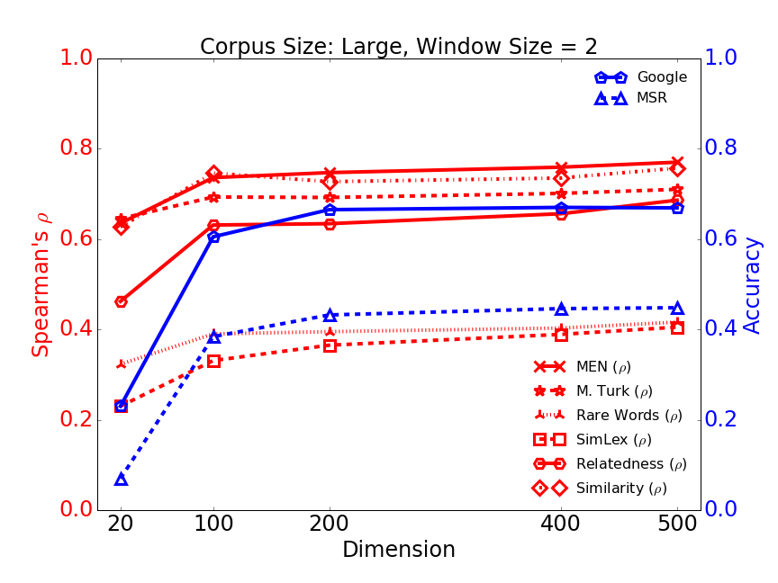
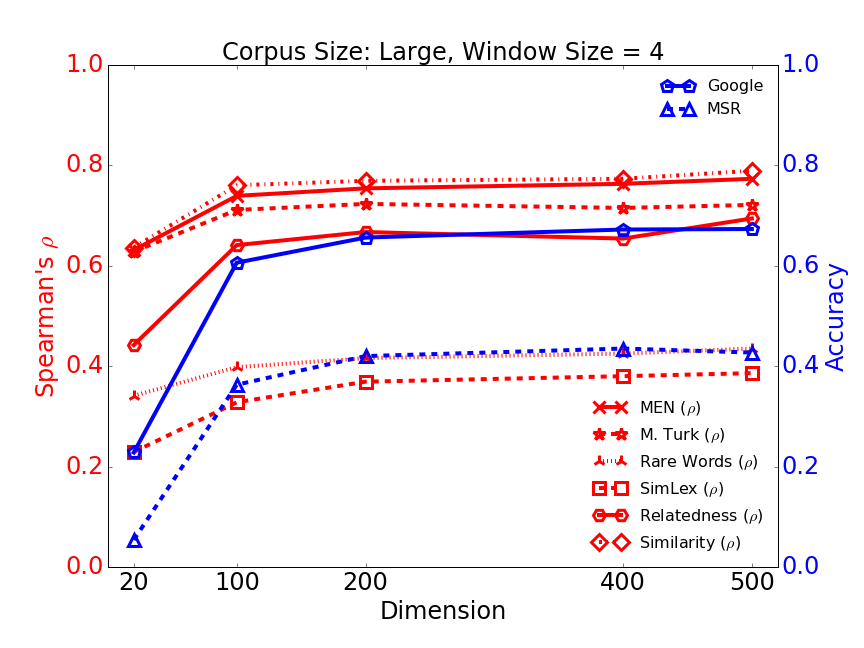
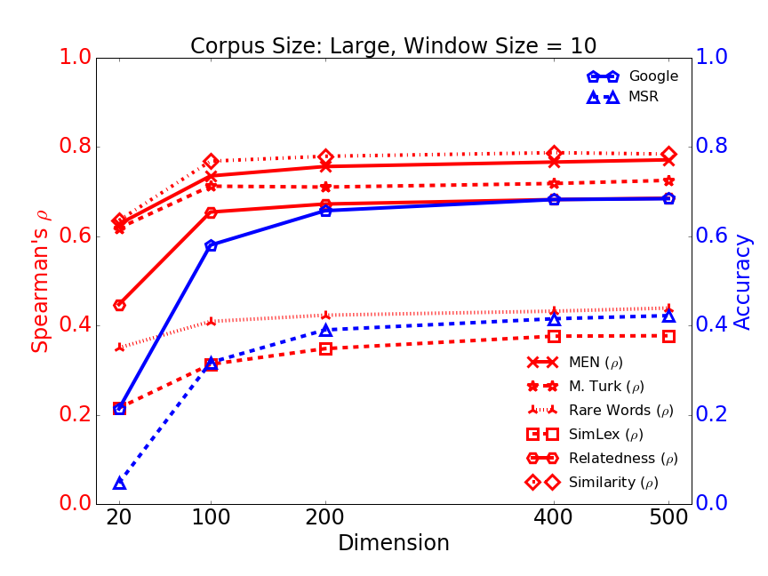
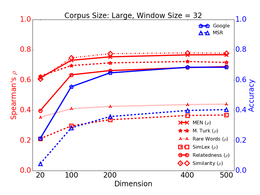
In all plots to follow, red lines denote word similarity evaluation performance, and blue lines denote analogy performance. For both evaluations, out-of-vocabulary words are discarded.

4.1 Varying Window Sizes

The window size hyper-parameter controls the number of contextual words surrounding a target word. The window size varied from 1 to 32. Results are presented in Figures 1 (corpus size $=$ small) and 2 (corpus size $=$ large)

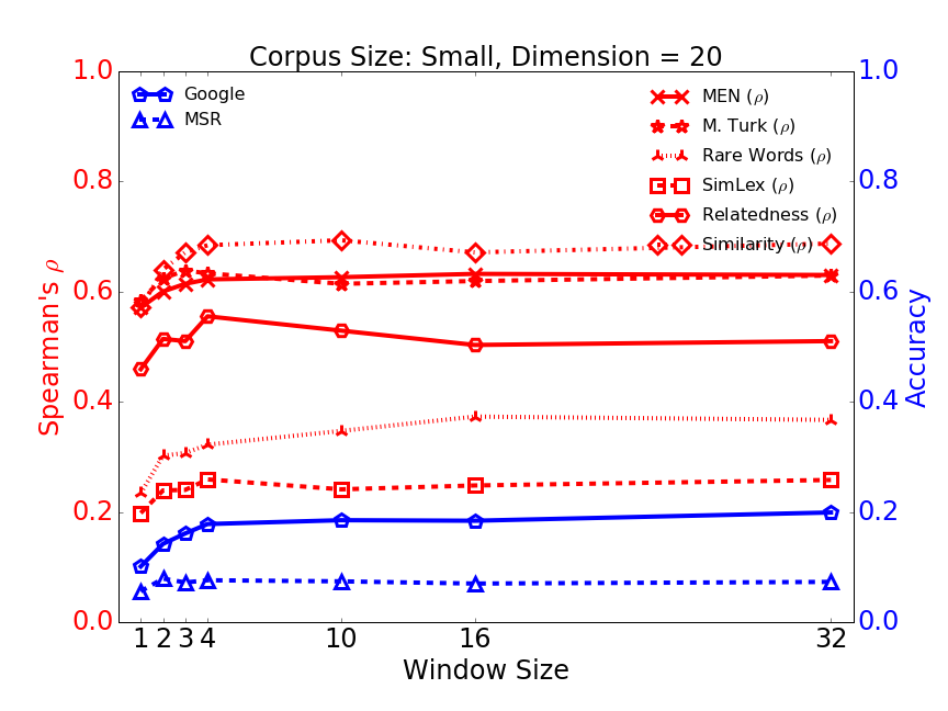
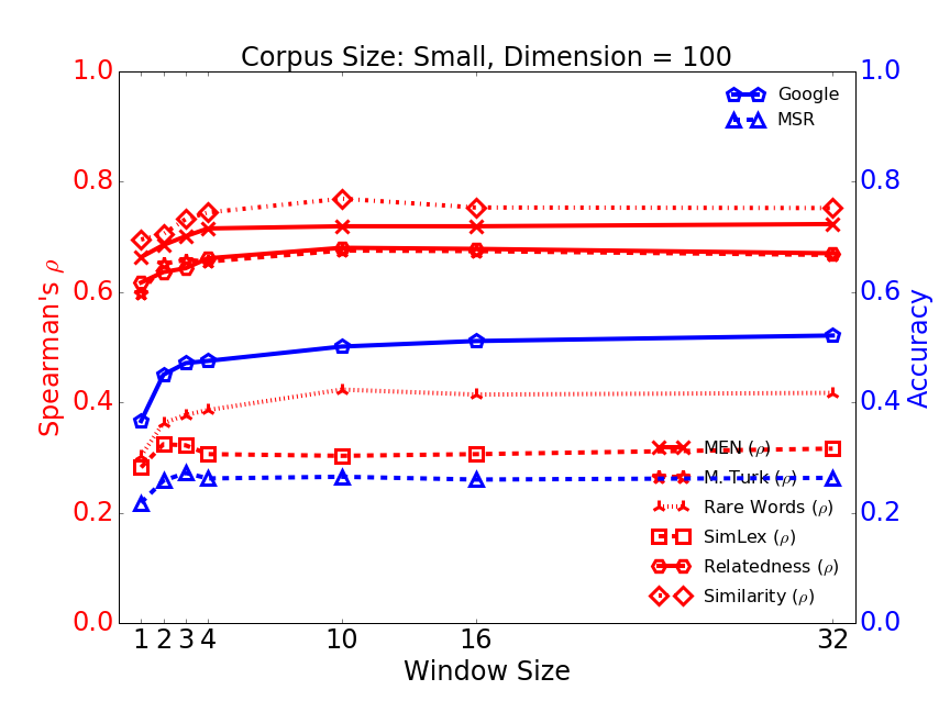
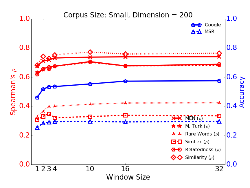
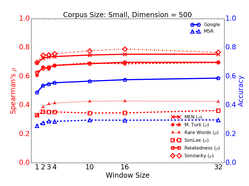
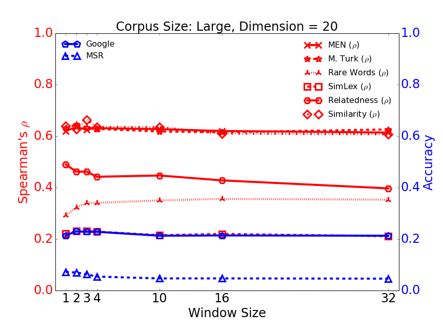
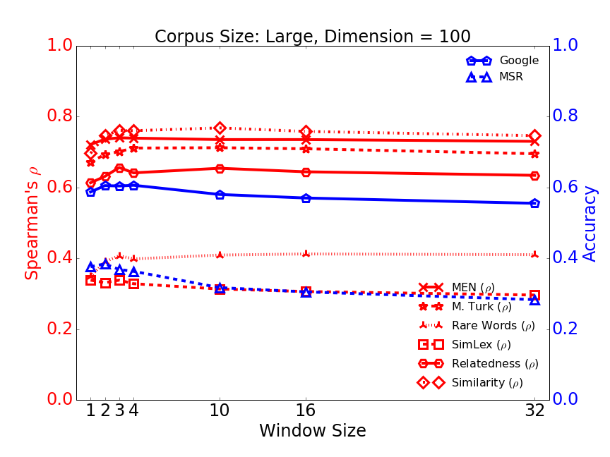
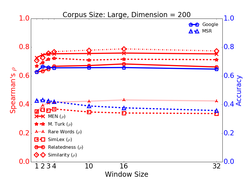
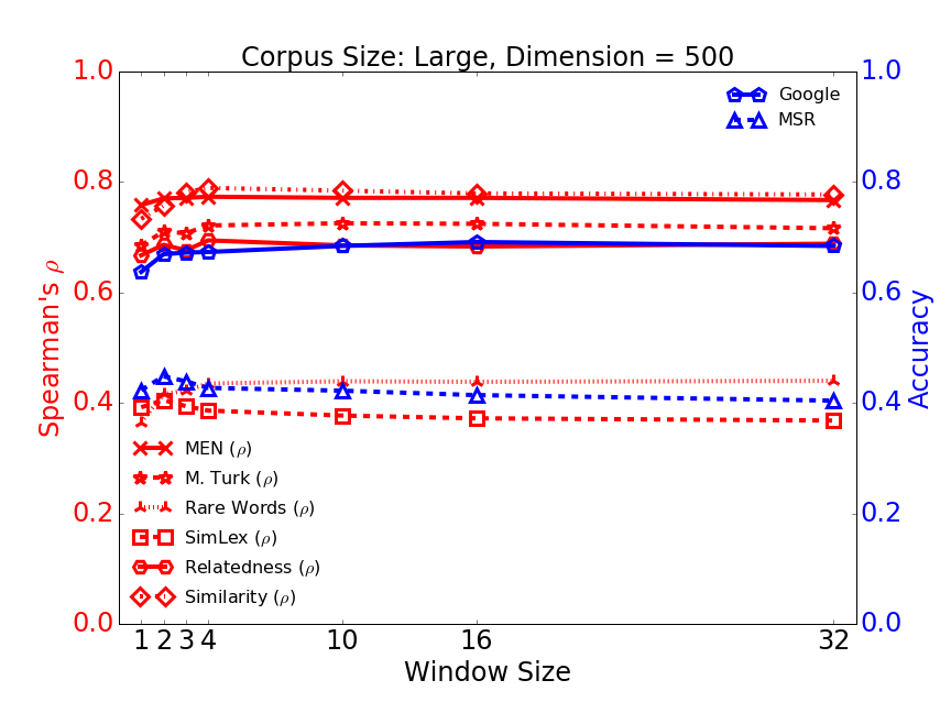
In each figure, results for varying vector dimension sizes are also shown. In general, it was found that there was little difference for both the similarity and analogy tasks when window size was greater than 4. This implies that increasing the window size beyond 4 does not have a significant impact on the performance in either task.

4.2 Varying Dimension Sizes

The dimension of the vectors was varied from 20 to 500; results are presented in Figure 3 (corpus size $=$ large). Largely similar results were observed with all corpus sizes; for brevity results using only the large corpus are presented.

The performance changes very little when dimension $=200$ was reached, with the exception of the analogy tasks where a small improvement was observed when the window size was greater than 4. These finding could be useful in situations where computational resources are limited, as it suggests that increasing the embedding dimension (and thus the number of parameters) does not necessarily translate to improved performance.

4.3 Varying Corpus/Token Sizes

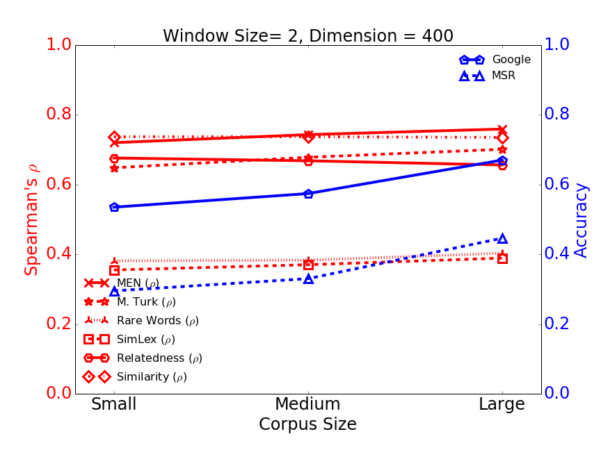
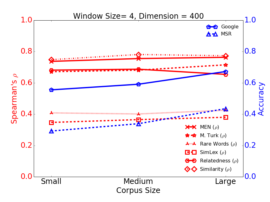
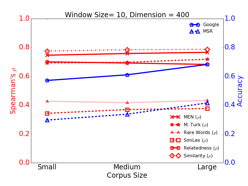
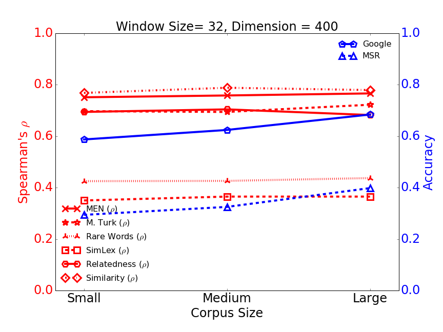
The corpus size used to train Swivel was varied (Table 1), the resulting performance on the similarity and analogy tasks are presented in Figure 4.

Interestingly, for the word similarity tasks, models trained using a small corpus (with less than 800K tokens) perform almost just as well as those trained using larger corpora. The word analogy tasks, however, benefit from a larger training corpora. This observation is not dissimilar to those found by previous studies [Chiu et al., 2016, Faruqui et al., 2016], where different tasks may favour different optimal hyper-parameter settings and embedding methodologies.

5 Discussion

In this paper, we conducted an empirical evaluation of the affect several hyper-parameter settings have on the performance of word embeddings. The evaluation was based on standard tasks commonly used in embedding evaluation, and all experiments were performed using word embeddings produced by Swivel, a competitive embedding model. The hyper-parameters explored were window size, vector dimension size and corpus size, and find interesting observations. For similarity tasks, increasing the amount of training data has a minimal impact on improving performance. For other tasks such as the analogy tasks, however, the accuracy increases with increased amounts of training data. In general, these hyper-parameters have a window of values that produce optimal performance, and that increasing these values beyond the window produces little or no performance improvement. These findings will be useful in situations where computational resources are limited or dataset size is constrained, providing insights for acceptable lower bound values for these hyper-parameters.

References

[Agirre et al., 2009] Eneko Agirre, Enrique Alfonseca, Keith B. Hall, Jana Kravalova, Marius Pasca, and Aitor Soroa. 2009. A study on similarity and relatedness using distributional and wordnet-based approaches. In Human Language Technologies: Conference of the North American Chapter of the Association of Computational Linguistics, Proceedings, May 31 - June 5, 2009, Boulder, Colorado, USA, pages 19–27.
[Bengio et al., 2003] Y. Bengio, R. Ducharme, P. Vincent, and C. Janvin. 2003. A neural probabilistic language model. The Journal of Machine Learning Research, 3:1137–1155.
[Bruni et al., 2012] Elia Bruni, Gemma Boleda, Marco Baroni, and Nam-Khanh Tran. 2012. Distributional semantics in technicolor. In Proceedings of the 50th Annual Meeting of the Association for Computational Linguistics: Long Papers-Volume 1, pages 136–145. Association for Computational Linguistics.
[Chiu et al., 2016] Billy Chiu, Anna Korhonen, and Sampo Pyysalo. 2016. Intrinsic evaluation of word vectors fails to predict extrinsic performance. In RepEval@ACL2016, The First Workshop on Evaluating Vector Space Representations for NLP, volume 1.
[Faruqui et al., 2016] Manaal Faruqui, Yulia Tsvetkov, Pushpendre Rastogi, and Chris Dyer. 2016. Problems with evaluation of word embeddings using word similarity tasks. CoRR, abs/1605.02276.
[Finkelstein et al., 2001] Lev Finkelstein, Evgeniy Gabrilovich, Yossi Matias, Ehud Rivlin, Zach Solan, Gadi Wolfman, and Eytan Ruppin. 2001. Placing search in context: The concept revisited. In Proceedings of the 10th international conference on World Wide Web, pages 406–414. ACM.
[Frome et al., 2013] Andrea Frome, Greg S Corrado, Jon Shlens, Samy Bengio, Jeff Dean, Marc Aurelio Ranzato, and Tomas Mikolov. 2013. DeViSE: A deep visual-semantic embedding model. pages 2121–2129.
[Gladkova and Drozd, 2016] Anna Gladkova and Aleksandr Drozd. 2016. Intrinsic evaluations of word embeddings: What can we do better? In RepEval@ACL2016, The First Workshop on Evaluating Vector Space Representations for NLP, volume 1.
[Hill et al., 2015] Felix Hill, Roi Reichart, and Anna Korhonen. 2015. Simlex-999: Evaluating semantic models with (genuine) similarity estimation. Computational Linguistics, 41(4):665–695.
[Levy and Goldberg, 2014] O. Levy and Y. Goldberg. 2014. Neural word embedding as implicit matrix factorization. pages 2177–2185, Montreal, Canada.
[Levy et al., 2015] Omer Levy, Yoav Goldberg, and Ido Dagan. 2015. Improving distributional similarity with lessons learned from word embeddings. Transactions of the Association for Computational Linguistics, 3:211–225.
[Li et al., 2014] Peng Li, Yang Liu, Maosong Sun, Tatsuya Izuha, and Dakun Zhang. 2014. A neural reordering model for phrase-based translation. pages 1897–1907, Dublin, Ireland.
[Linzen, 2016] Tal Linzen. 2016. Issues in evaluating semantic spaces using word analogies. In RepEval@ACL2016, The First Workshop on Evaluating Vector Space Representations for NLP, volume 1.
[Luong et al., 2013] Thang Luong, Richard Socher, and Christopher D. Manning. 2013. Better word representations with recursive neural networks for morphology. In Proceedings of the Seventeenth Conference on Computational Natural Language Learning, CoNLL 2013, Sofia, Bulgaria, August 8-9, 2013, pages 104–113.
[Mikolov et al., 2013a] Tomas Mikolov, Kai Chen, Greg Corrado, and Jeffrey Dean. 2013a. Efficient estimation of word representations in vector space. CoRR, abs/1301.3781.
[Mikolov et al., 2013b] Tomas Mikolov, Ilya Sutskever, Kai Chen, Gregory S. Corrado, and Jeffrey Dean. 2013b. Distributed representations of words and phrases and their compositionality. In Advances in Neural Information Processing Systems 26: 27th Annual Conference on Neural Information Processing Systems 2013. Proceedings of a meeting held December 5-8, 2013, Lake Tahoe, Nevada, United States., pages 3111–3119.
[Pennington et al., 2014] Jeffrey Pennington, Richard Socher, and Christopher D. Manning. 2014. Glove: Global vectors for word representation. In Proceedings of the 2014 Conference on Empirical Methods in Natural Language Processing, EMNLP 2014, October 25-29, 2014, Doha, Qatar, A meeting of SIGDAT, a Special Interest Group of the ACL, pages 1532–1543.
[Radinsky et al., 2011] Kira Radinsky, Eugene Agichtein, Evgeniy Gabrilovich, and Shaul Markovitch. 2011. A word at a time: computing word relatedness using temporal semantic analysis. In Proceedings of the 20th International Conference on World Wide Web, WWW 2011, Hyderabad, India, March 28 - April 1, 2011, pages 337–346.
[Řehůřek and Sojka, 2010] Radim Řehůřek and Petr Sojka. 2010. Software Framework for Topic Modelling with Large Corpora. In Proceedings of the LREC 2010 Workshop on New Challenges for NLP Frameworks, pages 45–50, Valletta, Malta, May. ELRA. http://is.muni.cz/publication/884893/en.
[Schnabel et al., 2015] Tobias Schnabel, Igor Labutov, David M. Mimno, and Thorsten Joachims. 2015. Evaluation methods for unsupervised word embeddings. In Proceedings of the 2015 Conference on Empirical Methods in Natural Language Processing, EMNLP 2015, Lisbon, Portugal, September 17-21, 2015, pages 298–307.
[Shazeer et al., 2016] Noam Shazeer, Ryan Doherty, Colin Evans, and Chris Waterson. 2016. Swivel: Improving embeddings by noticing what’s missing. arXiv preprint arXiv:1602.02215.
[Zesch et al., 2008] Torsten Zesch, Christof Müller, and Iryna Gurevych. 2008. Using wiktionary for computing semantic relatedness. In Proceedings of the Twenty-Third AAAI Conference on Artificial Intelligence, AAAI 2008, Chicago, Illinois, USA, July 13-17, 2008, pages 861–866.
[Zhang et al., 2014] Jiajun Zhang, Shujie Liu, Mu Li, Ming Zhou, and Chengqing Zong. 2014. Bilingually-constrained phrase embeddings for machine translation. pages 111–121, Baltimore, USA.

Appendix A Supplementary Material

All the results of the experimental study and evaluation has been shown in Table LABEL:table:results for further analysis and comparison.

Table 3: Results.

Data Size	Wind. Size	Dim. Size	MEN	M. Turk	Rare Words	SimLex	Relatedness	Similarity	Google	MSR
S	1	20	0.571	0.584	0.234	0.198	0.459	0.571	0.101	0.056
S	1	100	0.663	0.597	0.303	0.282	0.617	0.695	0.366	0.218
S	1	200	0.676	0.634	0.328	0.307	0.619	0.683	0.460	0.254
S	1	400	0.681	0.646	0.323	0.318	0.623	0.701	0.497	0.259
S	1	500	0.692	0.608	0.331	0.330	0.627	0.696	0.487	0.256
S	2	20	0.600	0.624	0.302	0.239	0.514	0.640	0.142	0.079
S	2	100	0.685	0.651	0.362	0.324	0.636	0.705	0.450	0.258
S	2	200	0.710	0.652	0.365	0.330	0.657	0.743	0.517	0.284
S	2	400	0.720	0.648	0.381	0.355	0.676	0.737	0.535	0.295
S	2	500	0.724	0.666	0.388	0.354	0.654	0.747	0.535	0.277
S	3	20	0.614	0.638	0.307	0.240	0.510	0.671	0.161	0.072
S	3	100	0.701	0.658	0.377	0.322	0.643	0.732	0.471	0.272
S	3	200	0.718	0.654	0.398	0.349	0.669	0.729	0.534	0.290
S	3	400	0.732	0.679	0.398	0.349	0.671	0.749	0.550	0.293
S	3	500	0.735	0.651	0.408	0.352	0.663	0.749	0.546	0.289
S	4	20	0.622	0.633	0.322	0.259	0.555	0.684	0.178	0.076
S	4	100	0.715	0.655	0.386	0.306	0.661	0.744	0.475	0.262
S	4	200	0.731	0.674	0.400	0.321	0.675	0.753	0.535	0.294
S	4	400	0.737	0.671	0.408	0.347	0.681	0.748	0.555	0.292
S	4	500	0.737	0.676	0.414	0.353	0.675	0.757	0.555	0.287
S	10	20	0.626	0.614	0.347	0.241	0.529	0.693	0.185	0.074
S	10	100	0.719	0.675	0.423	0.303	0.680	0.769	0.501	0.265
S	10	200	0.737	0.702	0.414	0.329	0.706	0.772	0.553	0.296
S	10	400	0.746	0.693	0.427	0.343	0.700	0.775	0.571	0.296
S	10	500	0.747	0.692	0.427	0.345	0.687	0.777	0.566	0.296
S	16	20	0.632	0.619	0.373	0.248	0.503	0.671	0.184	0.070
S	16	100	0.719	0.674	0.414	0.306	0.678	0.753	0.511	0.260
S	16	200	0.739	0.677	0.422	0.338	0.677	0.758	0.572	0.292
S	16	400	0.748	0.688	0.433	0.346	0.705	0.784	0.581	0.299
S	16	500	0.753	0.687	0.429	0.346	0.697	0.789	0.576	0.295
S	32	20	0.630	0.629	0.367	0.258	0.510	0.687	0.199	0.073
S	32	100	0.723	0.667	0.417	0.316	0.670	0.752	0.521	0.263
S	32	200	0.740	0.681	0.424	0.334	0.688	0.764	0.575	0.297
S	32	400	0.751	0.697	0.425	0.350	0.694	0.768	0.587	0.294
S	32	500	0.753	0.695	0.425	0.363	0.697	0.766	0.587	0.297
M	1	20	0.606	0.597	0.290	0.229	0.512	0.626	0.143	0.068
M	1	100	0.689	0.648	0.332	0.285	0.612	0.683	0.448	0.275
M	1	200	0.706	0.658	0.360	0.315	0.599	0.696	0.522	0.311
M	1	400	0.716	0.649	0.355	0.341	0.638	0.684	0.529	0.309
M	1	500	0.724	0.639	0.363	0.354	0.630	0.714	0.531	0.293
M	2	20	0.635	0.627	0.343	0.256	0.534	0.672	0.175	0.069
M	2	100	0.721	0.674	0.374	0.322	0.636	0.756	0.509	0.299
M	2	200	0.732	0.689	0.387	0.348	0.643	0.715	0.560	0.321
M	2	400	0.743	0.678	0.383	0.370	0.668	0.737	0.574	0.330
M	2	500	0.745	0.682	0.401	0.374	0.665	0.765	0.572	0.333
M	3	20	0.635	0.637	0.351	0.245	0.509	0.678	0.186	0.071
M	3	100	0.719	0.681	0.385	0.333	0.677	0.759	0.533	0.302
M	3	200	0.739	0.664	0.407	0.353	0.674	0.764	0.576	0.341
M	3	400	0.749	0.687	0.397	0.366	0.672	0.756	0.592	0.342
M	3	500	0.751	0.659	0.412	0.380	0.686	0.782	0.587	0.338
M	4	20	0.635	0.643	0.347	0.247	0.492	0.660	0.195	0.072
M	4	100	0.728	0.680	0.400	0.330	0.667	0.752	0.533	0.312
M	4	200	0.743	0.694	0.399	0.357	0.684	0.756	0.590	0.336
M	4	400	0.755	0.681	0.401	0.365	0.687	0.781	0.591	0.339
M	4	500	0.761	0.688	0.410	0.386	0.697	0.793	0.595	0.344
M	10	20	0.632	0.636	0.361	0.254	0.513	0.681	0.200	0.060
M	10	100	0.731	0.688	0.415	0.315	0.664	0.745	0.545	0.286
M	10	200	0.750	0.684	0.419	0.351	0.689	0.769	0.600	0.325
M	10	400	0.758	0.697	0.417	0.369	0.692	0.784	0.610	0.337
M	10	500	0.762	0.697	0.422	0.366	0.701	0.795	0.610	0.334
M	16	20	0.623	0.610	0.364	0.244	0.481	0.656	0.208	0.068
M	16	100	0.729	0.687	0.419	0.318	0.682	0.773	0.548	0.289
M	16	200	0.748	0.678	0.422	0.346	0.691	0.781	0.598	0.322
M	16	400	0.762	0.694	0.425	0.369	0.691	0.776	0.612	0.333
M	16	500	0.763	0.704	0.429	0.363	0.699	0.791	0.619	0.324
M	32	20	0.627	0.606	0.357	0.247	0.467	0.656	0.211	0.057
M	32	100	0.727	0.688	0.414	0.304	0.655	0.752	0.553	0.279
M	32	200	0.745	0.688	0.419	0.348	0.684	0.775	0.608	0.326
M	32	400	0.758	0.694	0.426	0.365	0.704	0.788	0.624	0.325
M	32	500	0.763	0.692	0.423	0.367	0.702	0.795	0.622	0.328
L	1	20	0.620	0.631	0.292	0.222	0.490	0.640	0.214	0.072
L	1	100	0.721	0.671	0.349	0.338	0.613	0.696	0.587	0.376
L	1	200	0.727	0.670	0.347	0.353	0.627	0.707	0.628	0.428
L	1	400	0.752	0.692	0.374	0.376	0.639	0.712	0.641	0.443
L	1	500	0.758	0.685	0.365	0.392	0.667	0.733	0.637	0.423
L	2	20	0.635	0.645	0.323	0.230	0.462	0.627	0.230	0.070
L	2	100	0.736	0.693	0.390	0.331	0.631	0.746	0.605	0.384
L	2	200	0.747	0.692	0.395	0.365	0.634	0.727	0.665	0.432
L	2	400	0.759	0.701	0.403	0.389	0.656	0.735	0.670	0.446
L	2	500	0.770	0.710	0.416	0.405	0.686	0.757	0.669	0.448
L	3	20	0.626	0.634	0.340	0.231	0.462	0.664	0.228	0.063
L	3	100	0.740	0.701	0.407	0.338	0.656	0.761	0.604	0.368
L	3	200	0.753	0.717	0.410	0.359	0.648	0.758	0.659	0.426
L	3	400	0.761	0.711	0.414	0.382	0.661	0.748	0.682	0.444
L	3	500	0.771	0.707	0.422	0.394	0.676	0.781	0.672	0.439
L	4	20	0.631	0.628	0.341	0.229	0.442	0.636	0.228	0.054
L	4	100	0.739	0.711	0.398	0.328	0.641	0.760	0.606	0.363
L	4	200	0.754	0.723	0.416	0.369	0.667	0.769	0.656	0.420
L	4	400	0.763	0.715	0.425	0.380	0.654	0.773	0.672	0.435
L	4	500	0.773	0.721	0.435	0.386	0.694	0.789	0.673	0.427
L	10	20	0.627	0.618	0.350	0.215	0.447	0.635	0.213	0.047
L	10	100	0.735	0.712	0.409	0.313	0.654	0.768	0.580	0.317
L	10	200	0.756	0.710	0.423	0.348	0.672	0.779	0.657	0.390
L	10	400	0.766	0.718	0.432	0.376	0.682	0.787	0.682	0.415
L	10	500	0.771	0.725	0.439	0.377	0.685	0.784	0.684	0.422
L	16	20	0.620	0.615	0.356	0.220	0.428	0.610	0.214	0.047
L	16	100	0.735	0.709	0.412	0.306	0.644	0.758	0.570	0.305
L	16	200	0.759	0.716	0.432	0.341	0.683	0.788	0.658	0.377
L	16	400	0.765	0.726	0.436	0.373	0.675	0.775	0.681	0.409
L	16	500	0.771	0.724	0.438	0.372	0.683	0.779	0.691	0.414
L	32	20	0.614	0.626	0.353	0.211	0.397	0.607	0.213	0.046
L	32	100	0.730	0.695	0.410	0.296	0.634	0.746	0.555	0.283
L	32	200	0.753	0.713	0.425	0.337	0.662	0.774	0.647	0.358
L	32	400	0.766	0.722	0.437	0.365	0.682	0.779	0.684	0.398
L	32	500	0.767	0.716	0.440	0.368	0.688	0.777	0.684	0.404

Table 3: Results. (continued)

Evaluating Word Embedding Hyper-Parameters for Similarity and Analogy Tasks