Semantic Exploration of Traffic Dynamics
Semantic Exploration of Traffic Dynamics
Abstract
Given a large collection of urban datasets, how can we find their hidden correlations? For example, New York City (NYC) provides open access to taxi data from year 2012 to 2015 with about half million taxi trips generated per day. In the meantime, we have a rich set of urban data in NYC including points-of-interest (POIs), geo-tagged tweets, weather, vehicle collisions, etc. Is it possible that these ubiquitous datasets can be used to explain the city traffic? Understanding the hidden correlation between external data and traffic data would allow us to answer many important questions in urban computing such as: If we observe a high traffic volume at Madison Square Garden (MSG) in NYC, is it because of the regular peak hour or a big event being held at MSG? If a disaster weather such as a hurricane or a snow storm hits the city, how would the traffic be affected?
While existing studies may utilize external datasets for prediction task, they do not explicitly seek for direct explanations from the external datasets. In this paper, we present our results in attempts to understand taxi traffic dynamics in NYC from multiple external data sources. We use four real-world ubiquitous urban datasets, including POI, weather, geo-tagged tweet, and collision records. To address the heterogeneity of ubiquitous urban data, we present carefully-designed feature representations for various datasets. Extensive experiments on real data demonstrate the explanatory power on taxi traffic by using external datasets. More specifically, our analysis suggests that POIs can well describe the regular traffic patterns. At the same time, geo-tagged tweets can explain irregular traffic caused by big events and weather can explain the abnormal traffic drop.
keywords:
Urban data, Traffic dynamics, RegressionThis manuscript is an extended version of the paper [Wu et al. (2016)].
This work is supported by the National Science Foundation, under grant #1618448 and #1544455. Author’s addresses: F. Wu, and H. Wang, and Z. Li, College of Information Sciences and Technology, Pennsylvania State University.
1 Introduction
Traffic is the pulse of the city that impacts daily life of millions of people. Traffic congestion can make drivers become frustrated and also generate a lot of city noises and vehicle accidents. Therefore, there has been a longstanding strong demand to understand and forecast traffic under different scenarios. An insightful analysis on traffic dynamics could lead to intelligent transportation systems that make the city flow more smooth and make people’s life easier.
Modeling traffic dynamics, however, is very difficult as the traffic varies significantly over space and time and it is impacted by many factors simultaneously. To date, various approaches have been proposed to model and to predict traffic [Zheng et al. (2014), Chan et al. (2012), Okutani and Stephanedes (1984), Xie et al. (2007), Van Der Voort et al. (1996), Chen et al. (2011), Abadi et al. (2015), Sun et al. (2006), Xu et al. (2014), Chen et al. (2014)] with or without considering external context datasets. But most of these studies focus on the prediction problem rather than seeking a direct explanation.
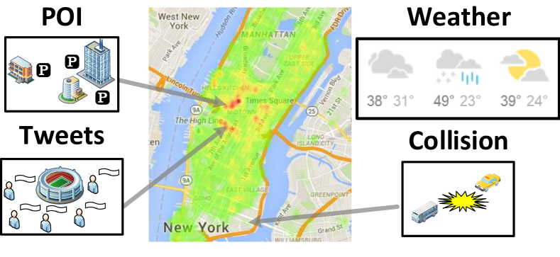
Motivated by this goal, we propose to study a novel problem: interpreting traffic data using external contextual urban data. Moreover, the big data era has brought us unprecedented urban data, which enables us to take a systematic approach to address this problem. Take New York City for example. The city generates about half million medallion taxi trips; all these data from year 2009 to year 2015 are publicly available on www.nyc.gov under the Freedom of Information Law (FOIL). The NYC taxi data was first made public in 2014. It is the first massive public traffic dataset which contains extremely rich information about the urban dynamics in NYC.
In the meantime, to understand such a large-scale traffic data, several contextual urban data in NYC are being collected from different sources. For example, information about more than 380K points-of-interest (POI) can be collected from FourSquare; people generate about half million geotagged tweets per day in the city; National Centers for Environmental Information provides daily climate information with 28 weather attributes collected from a monitoring tower in Central Park; more than 769K vehicle collisions from 2012 to today are available on NYC open data website (data.cityofnewyork.us). Our key insight is that all these ubiquitous urban datasets could potentially be valuable signals to explain the traffic dynamics: POIs describe the functions of a region (e.g., a business district always attracts a large volume of morning taxi drop-offs and evening taxi pick-ups; an area with many nightclubs has increased taxi drop-offs at night and pick-ups after midnight). Geo-tagged tweets capture local events (e.g., a popular event will generate peaks in drop-offs before the event and pick-ups after the event). Extreme weather could lead to traffic decline. Vehicle collisions might cause temporary road closures and traffic jams.
While all these urban datasets could potentially explain traffic dynamics, we face several key challenges when modeling the actual correlations: First, all these ubiquitous urban datasets are in different formats and contain different information. For example, POIs are mostly static and have categorical information such as POI categories as well as numeric information such as number of check-ins. Geo-tagged tweets are timestamped text. Weather information has a lower spatial and temporal granularity and also contains a large portion of missing values. Second, the relationship between traffic and the raw value of individual factor is unknown and non-linear. For example, most fluctuations of weather may not have a big impact on traffic unless it is an extreme weather; popularity of tweets might be associated with people tweeting about a popular global event (e.g., super bowl) and does not necessarily impact traffic. Furthermore, some factor (e.g., weather) may have impacts on top of other factors (e.g., POIs). For example, weather could have a damping impact on traffic but will not change the overall shape of the traffic time series, which is largely defined by the regional functions captured by the POIs.
To address these challenges, we study the properties of each dataset and capture their unique impacts by a carefully designed feature representations. We further propose a ridge regression model with polynomial kernel to describe the non-linear and non-additive relation between features. We quantitatively evaluate the effects of various datasets on traffic. Furthermore, qualitative investigations in selected regions lead to many interesting interpretations of the traffic dynamics. The analysis suggests that POI data are particularly good in capturing the regular traffic patterns, while tweets and weather are useful under certain occasions. And we do not observe significant impacts of collisions on taxi pick-ups and drop-offs. We also show that, by using external urban data only, one can infer the traffic condition more accurately compared to methods using historical traffic data only.
In summary, our paper has three major contributions:
-
•
We study a novel and important problem in urban computing: understanding traffic using ubiquitous urban data.
-
•
We investigate ways to design features and build models to capture the correlations between traffic and different types of urban data.
-
•
We conduct extensive experiments on five large-scale real datasets. The analysis provides insights on how external datasets can be used for interpreting taxi traffic.
The rest of the paper is organized as follow. We review the literature in Section 2. Section 3 describes the taxi dataset. Section 4 describes the contextual urban datasets that will be used to explain the taxi data and how we design features based on the properties of these datasets. Section 5 presents the ridge regression model with polynomial kernel. Section 6 presents the empirical evaluations of our method followed by a study of its application in traffic prediction. Section 7 discusses some interesting insights of our discoveries and limitations of the current method. And we conclude our work in Section 8.

2 Related Work
Trajectory prediction of moving objects. Quite a few previous studies [Monreale et al. (2009), Song et al. (2013), Song et al. (2014), Fan et al. (2015), Jeung et al. (2008), Song et al. (2010), Zheng and Ni (2012)] have been done on the problem of trajectory prediction. That is, given the historical trajectory traces of individual moving objects, predict the location for a future timestamp. The prediction is based on crowd behavior [Monreale et al. (2009), Song et al. (2013), Song et al. (2014), Fan et al. (2015)] or routine behaviors [Jeung et al. (2008), Song et al. (2010), Zheng and Ni (2012)]. Unlike this line of research on individual movements, our work focus on understanding the aggregated crowd traffic. The latter is very difficulty, more dynamic, computational expensive, and is important for urban issues such as transportation and public safety.
Traffic prediction. Traffic prediction has been extensively studied in transportation research area. Representative forecasting models include neural network models [Chan et al. (2012)], Kalman filters [Okutani and Stephanedes (1984), Xie et al. (2007)], autoregressive integrated moving average (ARIMA) models [Van Der Voort et al. (1996), Chen et al. (2011), Abadi et al. (2015)], Bayesian network approach [Sun et al. (2006), Xu et al. (2014)], and Markov Random Fields [Chen et al. (2014)].
Our problem and method are different from these studies in the following aspect. First, our problem is to model the correlation between traffic and external urban datasets instead of forecasting future traffic based on historical traffic data. Second, all these studies only consider one dataset – traffic data. The external factors that may have a huge impact on traffic are ignored. Our problem takes into consideration several large-scale urban datasets such as POI, geo-tagged tweets, weather, and vehicle collisions and study their impacts on traffic. Third, since our objective is not to predict future traffic based on history, the existing models cannot be applied. We need a different model to describe the complicated correlations with various impacting factors.
Computing with heterogeneous urban data. In recent years, urban computing [Zheng et al. (2014)] has gain an increasing popularity due to availability of large-scale urban data. These studies include using different urban datasets such as POI, taxi, bike rental, or noise complaint to profile city functions [Yuan et al. (2012)], detect traffic anomalies [Zheng et al. (2015b)], predict air quality [Zheng et al. (2013), Zheng et al. (2015a)], gas consumption [Shang et al. (2014)], and location recommendation [Lian et al. (2015)]. Our work is under the same theme of urban computing in the context of large-scale heterogeneous data. However, we distinctly put our emphasizes on understanding the traffic patterns from external sources.
3 Traffic Data
A large-scale New York City taxi dataset has been made public online [Government (2016)]. The dataset contains all trips completed in yellow and green taxis from 2009/01/01 to 2015/12/31. Each trip contains information about pick-up location and time, drop-off location and time, trip distance, fare amount, etc. We use the subset of trips from 2012/10/1 to 2012/12/31, which has trips. On average, we have trips per day. We pick this time period, as it aligns with the date of collection of other external context datasets. From the raw data, we make the following observations.
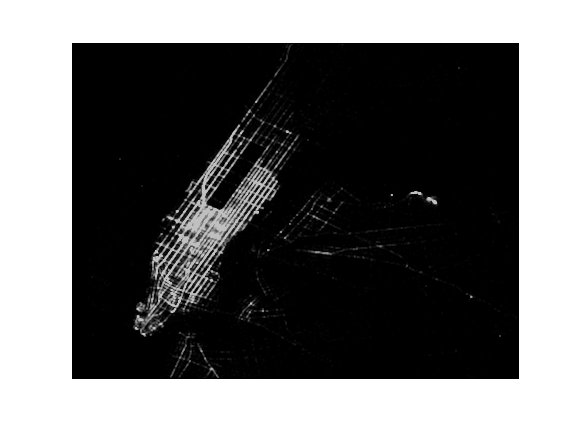
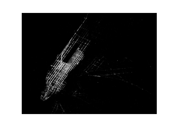
Traffic density changes over time. Figure 2 shows the distribution of GPS points of the pick-up and drop-off locations on different occasions. We can see that the traffic on holidays (e.g., Christmas as shown in Figure 2(b)) and under extreme weather condition (e.g., Hurricane Sandy as shown in Figure 2(c)) are significantly less compared with traffic in a normal day (as shown in Figure 2(a)).
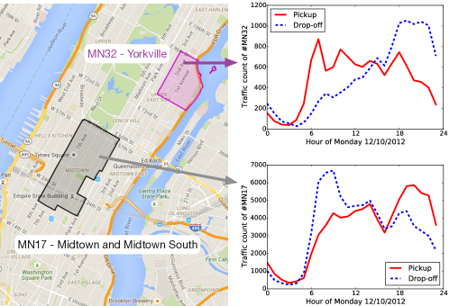
Different traffic patterns at different locations. Figure 3 shows that traffic patterns vary at different neighborhoods, as different neighborhoods have different functions. For Yorkville neighborhood (which is mainly consisted of residential area), we see a peak for pick-ups in the morning and a peak for drop-offs in the evening on weekday. For Midtown and Midtown South neighborhood, which mainly serves business purposes, a sharp peak for drop-offs appears in the morning whereas the peak for pick-ups occurs in the evening.
The observations indicates the potential correlations exist between traffic and contexts, e.g., weather and function of the region. In the following section, we further investigate several urban datasets and study their correlations between with the traffic.
4 Feature Design from Explanatory Urban Data
4.1 Point-of-Interest (POI) for Regional Functions
POI database provides us with rich information about the venues, which potentially correlates with the functionality of each location. Therefore, we gather a POI dataset from FourSquare [Fourquare (2016)]. The FourSquare API provides us venue information such as venue name, category, number of check-ins, and number of unique visitors. We focus on the major category information to characterize the neighborhood functions. There are 10 first-level categories in total: food, residence, travel, arts & entertainment, outdoors & recreation, college & education, nightlife, professional, shops, and event.
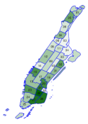
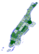
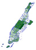
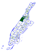
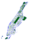
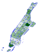
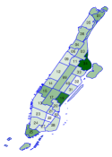
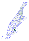
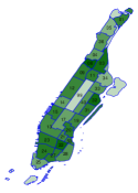
We query the FourSquare API to gather venues that are checked in by at least one user. In total, we get information about 380,380 venues for New York City. Figure 4 shows the number of unique users checked in to each category of the POIs for all neighborhoods in Manhattan area. The darker the color is, the higher the number. The color map suggests the degree of functions for each neighborhood with respect to a specific category. From Figure 4(a), we can see that majority of the users go to South East corner for nightlife. In Figure 4(c), POIs near Central Park are more related to arts entertainment.
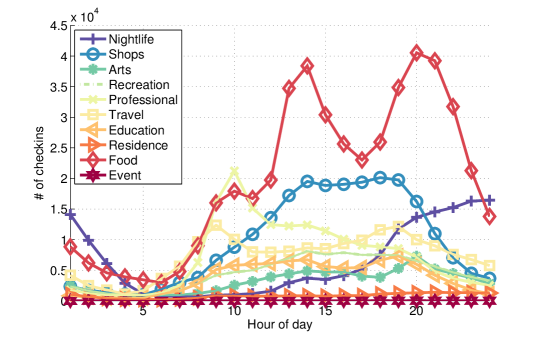
While the POI dataset enables us to model the overall functions of each region, it is important to consider the popularity over time for those categories. The time-varying popularity indicates the time span during which a region may be of interest to people. Therefore, we obtain dataset of FourSquare check-in posts from Twitter following the strategy introduced in [Noulas et al. (2011)]. We crawl geo-tagged tweets over the same time period, i.e., from Oct, 2012 to Dec, 2012. The check-in tweets start with “I’m at" followed by a venue name. A check-in tweet is matched with a POI if: (i) the geo-tag of the tweet is within 100 meters of the POI location, and (ii) similarity between POI names is large than 0.8, where the similarity is defined as the length of the longest common subsequence divided by the length of the longer sequence. As a result, we obtain check-ins. Later, the check-ins are aggregated by the POI category and by the hour of the day. Figure 5 shows the time-varying popularity (i.e., number of check-ins) of each category in each hour of the day. We can see that the popularity of food related venues peak at noon and early night times, while nightlife venues (e.g., bars) are more popular during night and have little attention during day time.
Given the two datasets, we define POI features for each region. Formally, let , , and denote the set of all categories, the set of all spatial grid cells, and the set of all timestamps, respectively. We consider a set of POIs on the map: . Each POI is represented as a tuple , where is the category of this POI, is its geographic location, and is the overall popularity of this POI measured by the total check-ins from FourSquare (this data is directly obtained from FourSquare API). We calculate the POI feature value for category in grid cell at time as:
| (1) |
where is the relative time (i.e., hour of the day) of , is the temporal popularity of the category at relative time of , i.e., shown in Figure 5. We adapt this hourly popularity definition for simplicity. There are other options for defining the temporal popularity, such as further differentiating between work day and non-work day, or aggregate the values at a different time granularity.
4.2 Geo-Tagged Tweets for Local Events
The POI features may help us capture the regular traffic at each location. To capture irregularity in traffic, we seek to extract event occurrences using geo-tagged tweets. Again we use the geo-tagged tweets dataset we collected in NYC around the same time period (from November, 2012 to Dec, 2012). Each geo-tagged tweet is of the form .
We count number number of unique users posting tweets that containing hashtags. Intuitively, local events should be identifiable via peaks in the space and time. Formally, we define the tweet feature value for a grid cell at time as:
| (2) |
where is the count of distinct users post a tweet at grid cell at time . We count the number of users instead of the posts to alleviate the problem of spammers. The number of users provides us a signal of population density at the location at the given time.
4.3 Weather for Disasters
Intuitively, the traffic should correlate with weather. Furthermore, extreme weather conditions such as hurricane and snow storm could significantly impact traffic. To capture the impact of weather, we use the daily weather dataset in USA from National Centers for Environmental Information [for Environmental Information (2016)]. There is one climate monitoring tower in Manhattan that situated in Central Park. The data contains 28 weather attributes for each day. We use the highest 2-mins wind speed, highest 5-seconds wind speed, precipitation, and snow fall information, as they are indicators for extreme weather in NYC.
Extreme weather conditions may have a lasting effect on traffic, as it may take days for recovering from damage. Therefore, we model the effect of extreme weather conditions by a power-law decaying function. Formally, we define the impact of an extreme weather event at time (after the event) on its corresponding weather feature as:
| (3) |
where and are positive values controlling the decay, is when event happens, and is the value of weather feature (corresponding to the extreme weather event) at time . is 0 for . When () the function decays slower (faster) at the beginning for a small time lag and gradually decays faster (slower). We let to capture the lasting effect of severe weather conditions.
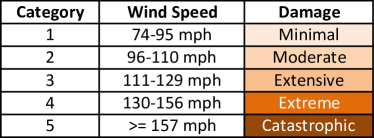
In practice, the values of , and depend on the severity of the weather conditions, the magnitudes of observed values, and the types of weather condition. We determine whether a severe weather event happens according to Saffir-Simpson hurricane wind scale [Center (2016)] on wind speed and according to Northeast Snowfall Impact Scale [Centers (2016)] on snowfall. In our experiment, we tune the two parameters to make the effect of extreme values last for three days. An example of wind scale categories and severity is shown in Figure 6. We also consider a severe weather event happens if the feature value is larger than ( and are mean and standard deviation of the feature values).
Finally, we can define weather features at time as:
| (4) |
where is set of all extreme weather events related to feature .
4.4 Vehicle Collisions for Traffic Jam
Vehicle collisions could potentially cause traffic controls on certain blocks and thus impact local traffic. Details of Motor Vehicle Collisions in New York City provided by the Police Department (NYPD) and can be accessed from NYC Open Data [Department (2016)]. This data is constantly being updated. From July 1st, 2012 to March 14th, 2016, there are about 769K collisions. To align with other datasets, we use data from the same period, i.e., from Oct, 2012 to Dec 2012.
Let denote the set of all collisions in our study. Each collision record is represented as a tuple , where the time of the collision, is the latitude and longitude of the collision, and is the number of people injured or killed in this collision. We construct our feature for collisions on day in grid cell using the number of collisions weighted by the severity of the collisions:
| (5) |
5 Model
We now present our approach to model the correlation between traffic and urban features. For each location grid , we denote the number of pick-up (or drop-off) at time as . The feature space is a combination of all the features:
Here, is a 10-dimensional feature because there are 10 categories for the POIs, and are one-dimensional features, and is -dimensional feature where depends on the number of weather attributes used. In our experiment setting, we use wind speed, precipitation, and snow fall. Given the data for a location grid , our goal is to fit a regression model for that grid.
Linear regression is arguably the most frequently used regression model in practice. It asserts that the response is a linear function of the inputs:
| (6) |
where and are the -th entry in the vectors and , respectively, is the dimension of the feature vector, and is a bias term.
To fit the model with training data, we need to find the parameter that minimizes the error:
| (7) |
A common technique to avoid overfitting is to control the values of weights on the features, where we add an -regularization to the objective function. In addition, the features may have multiplicative interactions among them. For example, in a bad weather day, the total traffic could decrease, but the relative traffic pattern over time (e.g., peak hours vs. non-peak hours) remains similar, which can be described by the temporal popularity of POIs. In this case, the traffic is determined as a combined effect of weather feature and POI feature. To avoid overfitting as well as consider the multiplicative effects, we use Kernel ridged regression (KRR) as our regression model.
6 Empirical Evaluation
In this section, we demonstrate the effectiveness of our approach with large-scale real world urban datasets. We first present the result of quantitative evaluation on our entire dataset. Later, we further conduct qualitative investigation on several regions of interest in hope of understanding how traffic data correlates with external datasets.
6.1 Quantitative Evaluation
Setting. We divide Manhattan into 500 meter 500 meter grids and build a model for each grid to predict hourly number of taxi pick-ups and drop-offs. There are 319 grids in the middle and lower area of Manhattan (i.e., South of street). Our experiments are conducted on these grids where the data from different sources are less sparse. Similar grid partition strategy has also been used in previous study [Zhang and Wang (2015)]. We use the first two weeks as training (from 10/01/2012 to 10/15/2012) to fit the model and use the next week for testing (from 10/16/2012 to 10/23/2012). The average hourly drop-off is 53 (pick-up is 56) for all grids and the standard deviation for hourly drop-off is 38 (pick-up is 41). The traffic also varies for different grids with the highest hourly drop-off being 926 (pick-up being 828) and lowest hourly drop-off (and pick-up) being 0.
We use mean-square error (MSE) and mean relative error (MRE) to evaluate testing error (on testing data) and coefficient of determination () to evaluate fitness of the model (on training data). Given a set of test samples , the rooted mean-square error is defined as: , where is the ground truth value, and is estimated value. The mean-relative error is defined as . The coefficient of determination is defined as . Note that the higher the value is, the better the data fit a model.
Feature effectiveness. P: POIs, T: geo-tagged tweets, W: weather, C: collision. RMSE, MRE and values are reported for different combination of features. all feature groups RMSE MRE
Feature Effectiveness. To study feature importance, we use leave-one-out strategy, that is, testing the model performance by excluding one feature from the feature set. Kernel ridge regression is the model used in this experiment.
Table 6.1 summaries the performance with different features (we only report the result for drop-off and the result of pick-up is similar). Without using POI features, RMSE is nearly two times larger than the model with POI features included, and MRE is three times larger. Similarly, is when excluding POI features, while is always higher than when POI features are used. The result suggests that POI features correlate the best with the taxi traffic data in general. At the same time, there is no significant improvement by including weather data, collision data, and tweet data. This is because traffic follows the routine behavior for most of the time, which is captured by POI features. Other features can describe abnormal scenarios (e.g., events and extreme weather), but such scenarios rarely happen or only happen in some small regions (e.g., convention center). When evaluating overall performance, these features become less important. However, these features are important in some cases at some specific locations. In the following sections, we qualitatively investigate several regions of interest to understand the correlation between traffic and these features.
6.2 Qualitative analysis
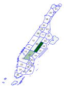
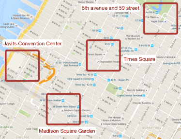
We manually select four regions for further inspection. We aim to pick a set of representative areas that cover different functions of a city, i.e., a tourist sight with entertainment related venues (Times Square), a big arena and a transportation center (Madison Square Garden, which sits on top of Penn Station), a central business area with many shops (5th avenue), and a large convention center (Jacob K. Javits Convention Center). Figure 7 shows the locations of the picked regions on a map. Each region is covered by an approximately 500 meter X 500 meter grid. We design our analysis with two questions in mind:
-
•
Q1 (Fitness): Can we construct the taxi traffic patterns by using external urban data?
-
•
Q2 (Interpretation): Which features are useful and under what circumstances they are useful?
To answer these two questions, we look at the fitting result of our model on all areas, as we want to know whether the external urban data can be used to explain the taxi traffic patterns. Using fitting result for explanatory purposes has also been seen in previous studies [Matsubara et al. (2014), Matsubara et al. (2015)] Figure 8 shows the fitting results for these four regions.


| (a) Madison Square Garden | (b) Times Square | (c) Fifth Avenue |
6.2.1 Traffic w.r.t. POIs.
Figure 8(a), (b), and (c) show the fitting results using our POI features for drop-offs and pick-ups at Madison Square Garden, Times Square, and 5th Avenue, respectively. In addition, we show the POI distribution (on discriminative categories) of these three regions in Figure 9. As one can see, in Madison Square Garden, categories “art” and “travel” dominate the distribution because Madison Square Garden hosts a lot of events and beneath that is Penn Station, one of the biggest transit center in NYC. We observe high traffic volume constantly from 7am to midnight because people transit through there all the time. For Times Square, category “art” is the biggest category because there are many theaters on Broadway. This explains why we see peaks for drop-offs and pick-ups around 8pm. Finally, 5th Avenue has a higher proportion of POIs in the “Shop” category. Therefore, we observe many drop-offs in the morning and pick-ups at 7pm (most shops close around 8pm – 9pm).
To further verify the external data indeed provide useful information, we generate 100-dimensional features with random values and use the same kernerlized ridge regression model to fit the traffic data (shown as blue dashed line in Figure 8(a), (b), and (c)). Obviously, these random features, although with a much higher dimension, cannot fit the traffic data well. This demonstrates the effectiveness of our POI features in explaining the traffic. The result also aligns with our quantitative experiment where POI features show strong correlation overall the regions.
6.2.2 Traffic w.r.t. Geo-tagged Tweets.
Geo-tagged tweets may help explain unexpected traffic patterns where local events are dominant source of traffic. Although overall geo-tagged tweets do not correlate with traffic, we found cases where traffic patterns can be attributed to ongoing events at a large-event venue, i.e., Javits center. As shown in Figure 8(d), we look at traffic data at Javits center during the period from 10/11/2012 to 10/13/2012, where there is large event, i.e., NYC Comic Con. It is clear that the considering geo-tagged tweets significantly improve the fitness of our model for event days.
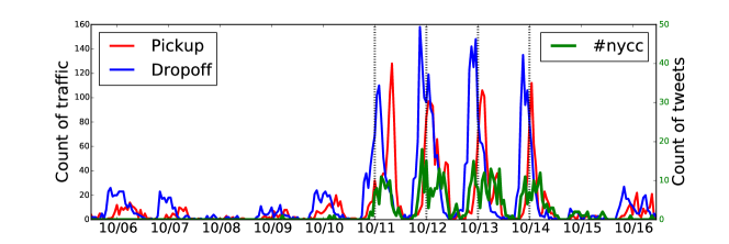
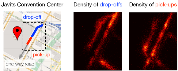
To verify the correlation, we look at time series of taxi traffic with the frequency of hastag “#nycc”. As shown in Figure 10, there is a strong correlation among these three time series. In Figure 11, we further observe that the drop-offs usually occur before the front entrance and pick-ups occurs after the front entrance.
6.2.3 Traffic w.r.t. Weather.
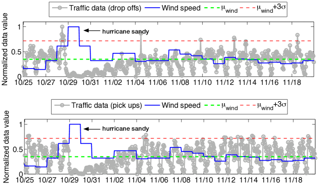
Intuitively, the extreme weather condition should impact the traffic. Here we particularly look at one weather event occurred during which time is covered by our datasets. Hurricane Sandy is a category-3 major hurricane that hit New York City on Oct. 29, 2012. The wind speed attribute in our weather feature captures the signal of this disaster. As shown in Figure 8(e), incorporating the weather information can effectively capture the significant drop of traffic volume during the time. By modelling the recovery time after the disaster, the fitted traffic pattern shows a slow recovery of traffic in the next 3 days, which aligns with the actual traffic pattern. Compared with not using the weather features, it demonstrates the utility of weather data in the presence of extreme weather conditions.
6.2.4 Insignificant Features.
While we found cases where many features have utilities in explain the traffic patterns, there are also features that have little impact on the traffic. We discuss two such features in this section, namely, the collisions and the snow fall.
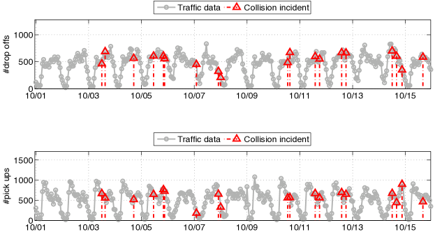
Common sense tells us that vehicle collisions cause blocking of road segments or traffic jam. Hence, there should be less pick-ups and drop-offs near the collision locations. However, we fail to see such a phenomenon in the taxi data. In Figure 13, we show one month of traffic at Madison Square Garden together with the vehicle collisions in that region. We do not observe any significant drop in traffic volume near the time of the collisions. The reason could be that, while the collisions do affect the local traffic, its impact is very subtle on the overall traffic (in terms of number of pick-ups and drop-offs). Capturing such minor impact using urban data still remains a challenging problem.
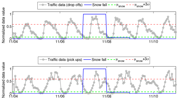
Meanwhile, from November 7 to November 10, 2012, a nor’easter brought significant snow to the Northeastern United States. Before the nor’easter struck, officials recommended residents in low-lying areas of New York City to evacuate. Airlines canceled over 1,300 flights in and out of New York airports. Parks in New York City were closed, and construction was halted. However, even though a high volume of snowfall was reported on Nov. 7th, as shown in Figure 14, the traffic volume exhibits similar patterns as normal days except that there is a slight drop in the afternoon on Nov. 7th. It is not certain whether such small variation in the traffic pattern is a result of the weather condition or due to the normal fluctuations of traffic.
6.3 Application: Regular Traffic Forecasting


A better modelling of traffic with contextual urban data can be used for traffic forecasting. In this section, we compare our approach with a forecasting method, autoregressive moving-average model (ARMA), that aims to capture the dynamics of traffic data with its own historical data. ARMA is commonly applied for time series fitting and forecasting. The model has two parameters and for its auto regressive and moving average component, respectively. Both parameters specify the range of previous values that a prediction depends on. In our setting, we set hours and . As urban data reflecting irregular events are hard to known beforehand, we only use POI features for the prediction and aim to predict the regular part of the traffic patterns.
Our method achieves better forecasting result, i.e., ARMA gives negative result, which indicates a very bad prediction result. Our approach consistently gives around for all locations. We further investigate the performance of both approaches for forecasting regular traffic. Figure 15 shows an example of forecasting result at Times Squares. We can see that the prediction of ARMA starts to converge and the peaks of the curve shift away from the actual data. ARMA performs poorly, as it is known to deteriorates when used to make predictions for a time point further into the future.
7 Discussion
7.1 Key Findings
Our results show that ubiquitous urban data can effectively explain the city traffic. Specifically, we have the observations:
-
•
POI data can well describe the regular traffic patterns in a local region. The result is shown both quantitatively and qualitatively.
-
•
Geo-tagged tweets may be related to traffic dynamics caused by the local events. However, such a correlation is more obvious in relatively isolated locations (e.g., Javits Convention Center, which locates on the west boundary of Manhattan).
-
•
Weather data are useful to describe natural disaster events. In particular, we observe hurricane Sandy from wind speed data and at the same time observe a significant drop of traffic volume in those days. However, not all the weather conditions have the same impacts. For example, the snow storm in November 2012 has a much smaller impact on the traffic compared to Sandy.
-
•
Vehicle collisions have little impact on hourly traffic. The reason could be (1) most collisions are minor accidents and do not have noticeable impact on traffic; (2) many major collisions happen on the highway or during the midnight, thus may not affect taxi pick-up and drop-off; (3) the temporal resolution we are currently using is hour but the collision impact may only last for a few minutes.
-
•
For insignificant changes in traffic, it is hard to tell whether the change is due to external impacts or to the normal fluctuations.
7.2 Limitations of Current Method
While most existing studies focus only on traffic data, our goal is to utilize ubiquitous urban datasets to interpret the traffic dynamics. But our finding may contain bias due to several limitations:
-
•
The traffic at one location may not be well explained by the external factors at the same location. There could be a cascaded effect of events at nearby locations. For example, if there is an accident on a major road in the morning peak hour, it may cause traffic jam on all in-bound routes. So a traffic jam does not mean that there is an accident at that particular location. In our currently analysis, we did not model such cascading effect.
-
•
We only consider traffic reflected by the numbers of drop-offs and pick-ups. Natural, the traffic can be expressed in other forms, such as the travel time and the speed of taxi trips. The correlation between some external factors with the traffic more become more obvious. For example, collisions could potentially slow down the traffic but not necessarily impact the volume.
-
•
Taxi traffic is only a subset of entire traffic in a city. Considering additional traffic data such as public transportation and private vehicles should provide us a more complete view. At the same time, the external context data may contain bias [Hecht and Stephens (2014)] as well, e.g., check-in data better reflect the behaviors of urban population rather than rural population. It is an interesting future direction to consider more comprehensive datasets.
-
•
Correlations do not necessarily indicate causality. For example, an event appears to correlate with the traffic, but people might be just going to other events at the same location. We plan to pursue a causality inference model, which provides us with more confident and more fine-grained interpretations.
8 Conclusion
We explored the potentials of using ubiquitous urban datasets to interpret traffic data. The traffic data we use are pick-up and drop-off of taxi trips in New York City. The explanatory urban datasets include POI data from FourSquare, geo-tagged tweets, weather, and vehicle collisions. We propose to use ridge regression with polynomial kernel to describe the non-linear non-additive relationships of impacting factors. Both quantitative and qualitative studies help us better understand the relation between traffic with its context. Additionally, we show an interesting application on traffic prediction using external urban datasets. Finally, we discuss the key insights of our results and limitations of current method. We conclude that using ubiquitous urban datasets helps us better understand the urban dynamics and could benefit a set of applications such as smart city and intelligent transportation system.
References
- [1]
- Abadi et al. (2015) Afshin Abadi, Tooraj Rajabioun, and Petros A Ioannou. 2015. Traffic flow prediction for road transportation networks with limited traffic data. Intelligent Transportation Systems, IEEE Transactions on 16, 2 (2015), 653–662.
- Center (2016) National Hurricane Center. 2016. Saffir-Simpson Hurricane Wind Scale. (2016). http://www.nhc.noaa.gov/aboutsshws.php.
- Centers (2016) NOAA’s National Centers. 2016. The Northeast Snowfall Impact Scale (NESIS). (2016). https://www.ncdc.noaa.gov/snow-and-ice/rsi/nesis.
- Chan et al. (2012) Kit Yan Chan, Tharam S Dillon, Jaipal Singh, and Elizabeth Chang. 2012. Neural-network-based models for short-term traffic flow forecasting using a hybrid exponential smoothing and Levenberg–Marquardt algorithm. Intelligent Transportation Systems, IEEE Transactions on 13, 2 (2012), 644–654.
- Chen et al. (2011) Chenyi Chen, Jianming Hu, Qiang Meng, and Yi Zhang. 2011. Short-time traffic flow prediction with ARIMA-GARCH model. In Intelligent Vehicles Symposium (IV), 2011 IEEE. IEEE, 607–612.
- Chen et al. (2014) Po-Ta Chen, Feng Chen, and Zhen Qian. 2014. Road traffic congestion monitoring in social media with hinge-loss Markov random fields. In Data Mining (ICDM), 2014 IEEE International Conference on. IEEE, 80–89.
- Department (2016) New York Police Department. 2016. Motor Vehicle Collisions. (2016). https://data.cityofnewyork.us/.
- Fan et al. (2015) Zipei Fan, Xuan Song, Ryosuke Shibasaki, and Ryutaro Adachi. 2015. CityMomentum: an online approach for crowd behavior prediction at a citywide level. In Proceedings of the 2015 ACM International Joint Conference on Pervasive and Ubiquitous Computing. ACM, 559–569.
- for Environmental Information (2016) NOAA’s National Centers for Environmental Information. 2016. http://www.ncdc.noaa.gov/. (2016).
- Fourquare (2016) Fourquare. 2016. https://foursquare.com/. (2016).
- Government (2016) NYC Government. 2016. NYC Taxi and Limousine Commission. (2016). http://www.nyc.gov/html/tlc/html/about/trip_record_data.shtml.
- Hecht and Stephens (2014) Brent Hecht and Monica Stephens. 2014. A Tale of Cities: Urban Biases in Volunteered Geographic Information. ICWSM 14 (2014), 197–205.
- Jeung et al. (2008) H. Jeung, H. T. Shen, and X. Zhou. 2008. Convoy Queries in Spatio-Temporal Databases. In Proc. 2008 Int. Conf. Data Engineering (ICDE’08). Cancun, Mexico, 1457–1459.
- Lian et al. (2015) Defu Lian, Yong Ge, Fuzheng Zhang, Nicholas Jing Yuan, Xing Xie, Tao Zhou, and Yong Rui. 2015. Content-Aware Collaborative Filtering for Location Recommendation Based on Human Mobility Data. In Data Mining (ICDM), 2015 IEEE International Conference on. IEEE, 261–270.
- Matsubara et al. (2015) Yasuko Matsubara, Yasushi Sakurai, and Christos Faloutsos. 2015. The web as a jungle: Non-linear dynamical systems for co-evolving online activities. In Proceedings of the 24th International Conference on World Wide Web. ACM, 721–731.
- Matsubara et al. (2014) Yasuko Matsubara, Yasushi Sakurai, Willem G Van Panhuis, and Christos Faloutsos. 2014. FUNNEL: automatic mining of spatially coevolving epidemics. In Proceedings of the 20th ACM SIGKDD international conference on Knowledge discovery and data mining. ACM, 105–114.
- Monreale et al. (2009) Anna Monreale, Fabio Pinelli, Roberto Trasarti, and Fosca Giannotti. 2009. Wherenext: a location predictor on trajectory pattern mining. In Proceedings of the 15th ACM SIGKDD international conference on Knowledge discovery and data mining. ACM, 637–646.
- Noulas et al. (2011) Anastasios Noulas, Salvatore Scellato, Cecilia Mascolo, and Massimiliano Pontil. 2011. Exploiting Semantic Annotations for Clustering Geographic Areas and Users in Location-based Social Networks. The social mobile web 11 (2011), 02.
- Okutani and Stephanedes (1984) Iwao Okutani and Yorgos J Stephanedes. 1984. Dynamic prediction of traffic volume through Kalman filtering theory. Transportation Research Part B: Methodological 18, 1 (1984), 1–11.
- Shang et al. (2014) Jingbo Shang, Yu Zheng, Wenzhu Tong, Eric Chang, and Yong Yu. 2014. Inferring gas consumption and pollution emission of vehicles throughout a city. In Proceedings of the 20th ACM SIGKDD international conference on Knowledge discovery and data mining. ACM, 1027–1036.
- Song et al. (2010) C. Song, Z. Qu, N. Blumm, and A. L. Barabasi. 2010. Limits of predictability in human mobility. In Science. 1018–1021.
- Song et al. (2013) Xuan Song, Quanshi Zhang, Yoshihide Sekimoto, Teerayut Horanont, Satoshi Ueyama, and Ryosuke Shibasaki. 2013. Modeling and probabilistic reasoning of population evacuation during large-scale disaster. In Proceedings of the 19th ACM SIGKDD international conference on Knowledge discovery and data mining. ACM, 1231–1239.
- Song et al. (2014) Xuan Song, Quanshi Zhang, Yoshihide Sekimoto, and Ryosuke Shibasaki. 2014. Prediction of human emergency behavior and their mobility following large-scale disaster. In Proceedings of the 20th ACM SIGKDD international conference on Knowledge discovery and data mining. ACM, 5–14.
- Sun et al. (2006) Shiliang Sun, Changshui Zhang, and Guoqiang Yu. 2006. A Bayesian network approach to traffic flow forecasting. Intelligent Transportation Systems, IEEE Transactions on 7, 1 (2006), 124–132.
- Van Der Voort et al. (1996) Mascha Van Der Voort, Mark Dougherty, and Susan Watson. 1996. Combining Kohonen maps with ARIMA time series models to forecast traffic flow. Transportation Research Part C: Emerging Technologies 4, 5 (1996), 307–318.
- Wu et al. (2016) Fei Wu, Hongjian Wang, and Zhenhui Li. 2016. Interpreting traffic dynamics using ubiquitous urban data. In Proceedings of the 24th ACM SIGSPATIAL International Conference on Advances in Geographic Information Systems. ACM, 69.
- Xie et al. (2007) Yuanchang Xie, Yunlong Zhang, and Zhirui Ye. 2007. Short-Term Traffic Volume Forecasting Using Kalman Filter with Discrete Wavelet Decomposition. Computer-Aided Civil and Infrastructure Engineering 22, 5 (2007), 326–334.
- Xu et al. (2014) Yanyan Xu, Qing-Jie Kong, Reinhard Klette, and Yuncai Liu. 2014. Accurate and interpretable Bayesian MARS for traffic flow prediction. Intelligent Transportation Systems, IEEE Transactions on 15, 6 (2014), 2457–2469.
- Yuan et al. (2012) Jing Yuan, Yu Zheng, and Xing Xie. 2012. Discovering regions of different functions in a city using human mobility and POIs. In Proceedings of the 18th ACM SIGKDD international conference on Knowledge discovery and data mining. ACM, 186–194.
- Zhang and Wang (2015) Wei Zhang and Jianyong Wang. 2015. Location and Time Aware Social Collaborative Retrieval for New Successive Point-of-Interest Recommendation. In Proceedings of the 24th ACM International on Conference on Information and Knowledge Management. ACM, 1221–1230.
- Zheng and Ni (2012) Jiangchuan Zheng and Lionel M Ni. 2012. An unsupervised framework for sensing individual and cluster behavior patterns from human mobile data. In Proceedings of the 2012 ACM Conference on Ubiquitous Computing. ACM, 153–162.
- Zheng et al. (2014) Yu Zheng, Licia Capra, Ouri Wolfson, and Hai Yang. 2014. Urban computing: concepts, methodologies, and applications. TIST 5, 3 (2014), 38.
- Zheng et al. (2013) Yu Zheng, Furui Liu, and Hsun-Ping Hsieh. 2013. U-Air: When urban air quality inference meets big data. In Proceedings of the 19th ACM SIGKDD international conference on Knowledge discovery and data mining. ACM, 1436–1444.
- Zheng et al. (2015a) Yu Zheng, Xiuwen Yi, Ming Li, Ruiyuan Li, Zhangqing Shan, Eric Chang, and Tianrui Li. 2015a. Forecasting Fine-Grained Air Quality Based on Big Data. In Proc. ACM SIGKDD.
- Zheng et al. (2015b) Yu Zheng, Huichu Zhang, and Yong Yu. 2015b. Detecting collective anomalies from multiple spatio-temporal datasets across different domains. Proc. 2015 ACM Int. Symp. Advances in Geographic Information Systems (GIS’15) (2015).