Low overhead Clifford gates from joint measurements in surface, color, and hyperbolic codes

Abstract

One of the most promising routes towards fault-tolerant quantum computation utilizes topological quantum error correcting codes, such as the $\mathbb{Z}_{2}$ surface code. Logical qubits can be encoded in a variety of ways in the surface code, based on either boundary defects, holes, or bulk twist defects. However proposed fault-tolerant implementations of the Clifford group in these schemes are limited and often require unnecessary overhead. For example, the Clifford phase gate in certain planar and hole encodings has been proposed to be implemented using costly state injection and distillation protocols. In this paper, we show that within any encoding scheme for the logical qubits, we can fault-tolerantly implement the full Clifford group by using joint measurements involving a single appropriately encoded logical ancilla. This allows us to provide new low overhead implementations of the full Clifford group in surface and color codes. It also provides the first proposed implementations of the full Clifford group in hyperbolic codes. We further use our methods to propose state-of-the art encoding schemes for small numbers of logical qubits; for example, for code distances $d=3,5,7$, we propose a scheme using $60,160,308$ (respectively) physical data qubits, which allow for the full logical Clifford group to be implemented on two logical qubits. To our knowledge, this is the optimal proposal to date, and thus may be useful for demonstration of fault-tolerant logical gates in small near-term quantum computers.

I Introduction

A crucial pillar of universal fault-tolerant quantum computation is the ability to perform quantum error correction Terhal (2015); Campbell et al. (2017). Schematically, given a physical qubit with an error probability $p$, a quantum error correcting code allows one to reach a target error rate for a logical qubit with error probability $p_{\text{fail}}\sim(p/p_{th})^{d/2}$, where $d$ is the code distance and $p_{th}$ is the error threshold of the codeFowler (2013a). It is therefore desirable to implement a code which maximizes $d$ and $p_{th}$ to the extent possible for a given set of physical resources. Codes that allow $d$ to be arbitrarily large while maintaining local interactions between the physical qubits are topological error correcting codes, which utilize the physics of topological states of matter Kitaev (2003); Wang (2008); Nayak et al. (2008). In topological error correcting codes on the Euclidean plane with local interactions, the ratio of the number of physical qubits $N_{phys}$ to the number of logical qubits $N_{L}$ scales as $N_{phys}/N_{L}=\mathcal{O}(d^{2})$ Bravyi et al. (2010).

The simplest topological error correcting code is known as the $\mathbb{Z}_{2}$ surface code Bravyi and Kitaev (1998); Dennis et al. (2002); Fowler et al. (2012a), and possesses a relatively high error threshold; for certain error models the error threshold is quoted to be $p_{th}\sim 1\%$Stephens (2014a). Given the rapid experimental advances in qubit technology using various physical platforms, it is reasonable to expect that the $\mathbb{Z}_{2}$ surface code will play an important role in near-term demonstrations of fault-tolerance. Closely related error correcting codes are the color codes Bombin and Martin-Delgado (2006) and hyperbolic codes Freedman et al. (2002); Breuckmann and Terhal (2016); Breuckmann et al. (2017). The color code is effectively two independent copies of the $\mathbb{Z}_{2}$ surface code Kubica et al. (2015); while it has a lower error thresholdStephens (2014b), it allows for transversal implementation of Clifford gates and improves the space-time overhead Landahl and Ryan-Anderson (2014). The hyperbolic codes are related to the $\mathbb{Z}_{2}$ surface code on a tiling of hyperbolic space; they allow one to improve the scaling of the ratio $N_{phys}/N_{L}$ to be independent of $d$, at the cost of requiring non-local interactionsBreuckmann and Terhal (2016).

As we review below, logical qubits can be encoded in the surface code in a number of different ways: through (1) boundary defects, which are domain walls between alternating boundary conditions, (2) holes, or (3) bulk twist defects. Hybrid approaches that combine any or all of the above are also possible.

The set of fault-tolerant logical operations that can be performed using the $\mathbb{Z}_{2}$ surface code form the Clifford group. In addition to Pauli operations on single qubits, this group is generated by the single qubit Hadamard gate $H$, phase gate $S$, and two-qubit CNOT gate. A variety of methods are known for implementing these gates in the $\mathbb{Z}_{2}$ surface code, however they depend sensitively on the encoding scheme Dennis et al. (2002); Fowler et al. (2012a); Horsman et al. (2012); Hastings and Geller (2014); Litinski and von Oppen (2017a); Yoder and Kim (2017); Brown et al. (2017). In particular, for the schemes that are based purely on boundary or hole defectsFowler et al. (2012a); Horsman et al. (2012), implementing the Clifford phase gate require a costly state distillation protocol with a large overhead that scales exponentially with the number of distillation rounds. The CNOT and $H$ gates in these encoding schemes also require unnecessary overhead, as we argue below. To avoid these overhead costs, various encoding scheme specific solutions have been devisedBrown et al. (2017); Litinski and von Oppen (2017a), which we will review briefly below.

In the past few years, an approach to topological quantum computation has been developed that utilizes the idea of topological charge measurements.Bonderson et al. (2009); Barkeshli and Freedman (2016) In particular, Ref. Barkeshli and Freedman, 2016 demonstrated that topological charge measurements along certain ‘graph’ operators could in principle be utilized to implement non-trivial fault-tolerant logical unitary gates (see also Ref. Cong et al., 2016).

In this paper, we demonstrate how to efficiently implement the full Clifford group with low overhead in the surface code, using any of the above encoding schemes for the logical qubits. Our method is based on fault-tolerantly implementing the necessary topological charge measurements using any logical encoding scheme in the surface code. Notably, this allows us to implement the Clifford phase gate in any encoding scheme without using costly state distillation protocols, and further allows implementation of $H$ gates and arbitrarily long-range CNOT gates with minimal overhead.

Our results can be applied not only to 2D surface codes in any logical encoding scheme, but also to 3D surface codes. We further apply our methods to both color codes and hyperbolic codes. In the context of hyperbolic codes, we provide the first proposed implementations of Clifford gates. In the context of color codes, we also propose novel efficient methods for implementing Clifford group operations in a hole based encoding scheme, which provides some advantages over alternate proposalsBombin and Martin-Delgado (2006); Landahl and Ryan-Anderson (2014); Litinski and von Oppen (2017b).

Finally, using these insights, we further present encoding schemes for small numbers of logical qubits that allow fault-tolerant implementation of the full Clifford group with minimal overhead in terms of number of physical qubits for a given code distance. This leads us to state-of-the art code designs that minimize number of physical qubits while allowing for all Clifford group operations to be implemented on two logical qubits. Specifically, for code distances $d=3,5,7$, we propose a scheme using $60,160,308$ (respectively) physical data qubits, which allow for the full logical Clifford group to be implemented on two logical qubits. To our knowledge, this is the optimal proposal to date, and thus may be useful for near-term experiments to demonstrate fault-tolerance.

We note that to obtain universal fault-tolerant quantum computation, the Clifford group must be supplemented with an additional gate, such as the single qubit $\pi/8$ phase gate. In the codes that we study in this paper, this gate inevitably requires magic state injection and distillation. In this paper we focus on efficient fault-tolerant implementations of gates in the Clifford group, and do not further consider the $\pi/8$ phase gate.

The rest of this paper is organized as follows. In Sec. II we provide a review of active error correction with the surface code, together with a brief review of the different encoding schemes and proposals for carrying out quantum computation with them. In Sec. III, we explain the abstract joint measurement circuits that allow implementation of the full Clifford group. In Sec. IV, we demonstrate how to implement these measurement circuits in the surface code, using two methods: with the aid of CAT states, or using a twist defect logical ancilla. In Secs. V-VI we further apply these results to hyperbolic and color codes. Finally in Sec. VII we provide resource overhead estimates in terms of the number of physical qubits required to carry out our proposal, and compare them to other existing proposals. In particular, we provide novel state-of-the-art proposals that minimize the number of physical qubits for small numbers of logical qubits, while allowing full implementation of the Clifford group. In Sec. VIII we provide some concluding remarks.

II Review of logical qubit encodings and Clifford gates in surface code

We begin with a brief review of the various proposalsDennis et al. (2002); Fowler et al. (2012a); Horsman et al. (2012); Hastings and Geller (2014); Yoder and Kim (2017) for quantum computing with the surface code.

II.1 Planar encoding

The simplest type of surface code is the planar code based on boundary defects.Bravyi and Kitaev (1998); Freedman and Meyer (2001); Dennis et al. (2002) We consider a physical qubit at each site of a square lattice, as shown in Fig. 1a. Each plaquette $p$ is associated with a stabilizer $S_{p}$, with dark plaquettes representing $X$ stabilizers and light plaquettes representing $Z$ stabilizers:

$$S_{p}=\prod_{i\in\partial p}\sigma_{i},\qquad\sigma=\begin{cases}X,&\text{if}\ p\ \text{is dark}\\ Z,&\text{if}\ p\ \text{is light},\end{cases}$$ (1)

where $\partial p$ denotes the boundary of the $p$ plaquette. In the bulk, the stabilizers have support on four physical qubits. Violations of $X$-type stabilizers are referred to as $e$ particles, and violations of $Z$-type stabilizers are referred to as $m$ particles. Local operators in the bulk can only create $e$ particles in pairs, and similarly for $m$ particles.

On the boundary, the stabilizers, shown as semicircles in Fig. 1a, involve two physical qubits. An edge with only $Z$ type stabilizers is referred to as an $e$ boundary, because applying a $Z$ operator on an edge qubit can create a single $e$ particle; therefore, the $e$ particles are ‘condensed’ on such an edge. Similarly, an edge with only $X$ type stabilizers is referred to as an $m$ boundary (see Fig. 1a). To avoid drawing the entire lattice, we use schematic diagrams whenever possible, as shown in Fig. 1b. The crosses on the edges, which are domain walls between the two types of boundaries, are referred to as boundary defects.

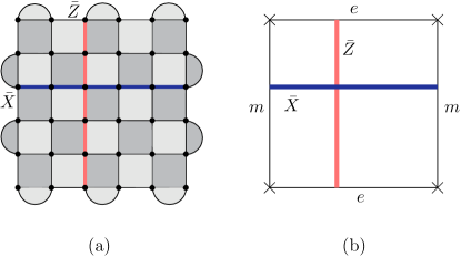
Figure 1: (Color online) a) A simple distance $6$ surface code encoding $1$ logical qubit. Black dots are physical qubits. Each dark(light) plaquette represents a $X$($Z$) stabilizer. The semicircles at the boundaries are also stabilizers that involve just two qubits. The logical $\bar{X}$ and $\bar{Z}$ operators are shown by horizontal blue (dark gray) and vertical red (light gray) strings respectively. b) Schematic diagram of the surface code in (a).

The stabilizers all commute with each other. The code space $\mathcal{C}$ is defined as the set of states that are eigenvectors of all stabilizer operators with eigenvalue $+1$:

$$\mathcal{C}=\quantity{\ket{\psi}:\,S_{p}\ket{\psi}=+\ket{\psi}\quad\forall p}.$$ (2)

The dimensionality of $\mathcal{C}$ determines how many logical qubits can be encoded in this surface code. For the lattice shown in Fig. 1a, there is one less stabilizer than physical qubits. Therefore $\mathcal{C}$ is two-dimensional and corresponds to the encoded logical qubit. It is possible to encode more than one logical qubit in one patch if one uses more defects on the boundary; $2n$ boundary defects can be used to encode $n-1$ logical qubits. However in the planar code, each logical qubit is associated with a separate patch.

Logical operators are associated with those unitary transformations which leave the code subspace $\mathcal{C}$ invariant, but which act non-trivially within $\mathcal{C}$. Logical Pauli operators $\bar{Z}$ and $\bar{X}$ correspond to a tensor product of Pauli operators for each physical qubit along a given string:

$$\bar{Z}=\prod_{i\in l}Z_{i},\qquad\bar{X}=\prod_{i\in l^{\prime}}X_{i},$$ (3)

where $l$ and $l^{\prime}$ are the light red and dark blue strings, respectively, depicted in Fig. 1a. The choice of $l$ and $l^{\prime}$ is unphysical; any string $l$ that connects the top and bottom edges is sufficient for $\bar{Z}$, and analogously for $\bar{X}$. Physically, $\bar{Z}$ corresponds to an $e$ particle being transported between the top and bottom edge, while $\bar{X}$ corresponds to an $m$ particle being transported between the left and right edge.

The distance of the code, $d$, is the minimum number of Pauli operators that appear in a nontrivial logical operator. Here, both $\bar{Z}$ and $\bar{X}$ have length $6$, hence it is a distance $d=6$ code.

II.1.1 Error correction in surface codes

Here we briefly review the proposal for active quantum error correction using the surface code. In this approach, all of the stabilizers $S_{p}$, for every plaquette, are measured in each round of quantum error correction. By constantly measuring the stabilizers $S_{p}$ for every plaquette, we can ensure that the state of the system remains an eigenstate of each stabilizer.

While each $S_{p}$ is a physical operator on four qubits, it can be measured using only two-qubit CNOT operations with the aid of a physical ancilla qubit, which can be placed at the center of each plaquette. To measure a stabilizer, such as $X_{1}X_{2}X_{3}X_{4}$, one can use the circuit shown in Fig. 2b Fowler et al. (2012a). The extra ancilla qubit used in this circuit is called the syndrome or measurement qubit. In Fig. 2c, a similar circuit is shown which is used to measure a typical $Z$ stabilizer.

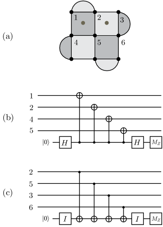
Figure 2: a) A distance $3$ planar code encoding one logical qubit. The gray dots in the center of plaquettes are the syndrome qubits for the corresponding stabilizer. b) & c) are quantum circuits used to measure a typical $X$ and $Z$ stabilizer respectively. Numbers represent physical qubits shown in (a).

Consider the planar code shown in Fig. 3. Let us say a bit flip error occurs on qubit number $1$ and the wave function of the system changes to $X_{1}\ket{\psi}$. Now, when we measure the stabilizers, assuming a perfect measurement, all syndromes would be $+1$ except for the measurement outcomes of $Z$ stabilizers marked by blue circles in Fig. 3, which will be $-1$. Thus a single bit flip error creates two adjacent $m$ particles. If instead of a bit flip, a phase flip error had happened, then it would be the $X$ stabilizers marked by red triangles adjacent to qubit $1$ that would give different output, giving rise to a pair of adjacent $e$ particles.

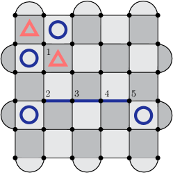
Figure 3: (Color online) Error syndromes can be used to detect and correct errors. A single bit flip error on qubit $1$ will create two neighboring $m$ particles indicated here by blue (dark gray) circles whereas a phase flip error will create two $e$ particles (shown as red (light gray) triangles). Error strings like the one shown at the bottom, can create isolated particles.

An arbitrary single qubit error on the qubit number $1$ would change the wave function of the system to:

$$e^{i\theta\bm{n}\cdot\bm{\sigma}_{1}}\ket{\psi}= \cos(\theta)\ket{\psi}+i\sin(\theta)n_{x}X_{1}\ket{\psi}$$

$$+i\sin(\theta)n_{y}Y_{1}\ket{\psi}+i\sin(\theta)n_{z}Z_{1}\ket{\psi}.$$ (4)

The four terms on the right hand side of Eq. 4 have different error syndromes and after one round of measurement, the system will collapse to one of them. So, from the standpoint of error correction, any single qubit error reduces to a bit flip or phase flip error, or a combination of the two.

If instead of a single qubit error, many adjacent qubits flip at the same time, only the syndromes at the end of the flipped string would give different values. Fig. 3 illustrates an example. An error string, such as $E=\prod_{i\in s}X_{i}$ for some string $i$, creates an $m$ particle at each end of the string. Similarly an error string consisting of Pauli-$Z$ errors creates a pair of $e$ particles at its ends. However if an error string ends on an appropriate boundary, such as a $Z$ error string that ends on an $e$ boundary, then only a single $e$ particle is created, and therefore only one stabilizer, at the endpoint of the string in the bulk, is violated.

Therefore, when an error occurs in the form of some strings, the only information we get from syndrome measurements is the position of the $e$ and $m$ particles. However, given a set of syndrome measurements (locations of $e$ and $m$ particles), the error string that can create it is non-unique; many different errors can result in the same configuration of particles. The minimum weight perfect-matching method Edmonds (1965a, b) can be used to track back the most likely error strings from the error syndromes. The method finds the set of shortest possible strings that connect a given set of particles. Since longer error strings occur with lesser probability, this algorithm finds the most probable error configuration consistent with the measured syndromes. A logical error occurs when the error string inferred from the minimum weight perfect matching algorithm differs from the correct error string by a non-contractible string. On the other hand, if the inferred error strings are always related to the true error strings by a contractible loop, then that means that we have successfully tracked all of the errors in the software and can compensate for them accordingly. Other variants of the matching algorithm can be used to improve the probability of guessing the true error configurationHeim et al. (2016); Baireuther et al. (2018).

Since the standard minimum weight matching algorithm runs in polynomial time in system size $l$, for large patches of surface code other methods like renormalization-group decoders with $\mathcal{O}(\log l)$ run time could become favourable Duclos-Cianci and Poulin (2010, 2013). Having enough classical resources, one can also solve the minimum weight matching problem in constant time using parallel computing Fowler (2013b).

The probability of a logical error $p_{\text{fail}}$ clearly depends on the underlying error model. For uncorrelated single qubit errors, numerical and analytical studies suggest an exponential suppression of $p_{\text{fail}}$ with increasing code distanceDennis et al. (2002); Wang et al. (2003); Fowler (2012, 2013a); Watson and Barrett (2014). The rate of exponential decay depends on the physical error probability. Specifically, for fixed $d$ and small probability of physical errors $p$, $p_{\text{fail}}$ is best described by $A(d)(p/p_{\text{th}})^{d/2}$ where $p_{\text{th}}$ is called the accuracy threshold Fowler (2012, 2013a); Wang et al. (2003); Fowler et al. (2012b). The same form applies for other variants of the surface code but with different values for $p_{\text{th}}$.

So far we have assumed that the measurement process is perfect. But one also needs to consider the errors that occur in the measurement process. Measurement errors can be addressed by repeating the measurements many times to distinguish the measurement errors from other errors. By repeating the measurement many times, we get a three dimensional map for the position of quasiparticles: two dimensions are used to record the error syndromes in space for each round of measurement and the third dimension is the discrete time. Now, we use the minimal weight perfect-matching algorithm to connect the quasiparticles in this three dimensional lattice together, allowing for the strings to have time segments as well as spatial onesFowler et al. (2012a, b).

The number of measurement histories that are used for error correction depends on the code distance and the probability of measurement errors. For equal error probability in measurement and storage, $\mathcal{O}(d)$ rounds of previous error syndromes are used to correct the code where $d$ is the code distanceRaussendorf et al. (2007); Fowler et al. (2012c).

II.1.2 Measuring string operators in planar codes

Here we will discuss how to fault-tolerantly measure the string operators associated with $\bar{X}$ and $\bar{Z}$. These methods can also be used for initializing logical qubits in the $\bar{X}$ or $\bar{Z}$ basis.

We note that one method to measure $\bar{X}$ and $\bar{Z}$ is to measure all physical qubits in the $X$ or $Z$ basis in order to measure the corresponding logical operator. However since this method is destructive it cannot be used when there are more than one logical qubits encoded in a patch. In contrast, the string measurement that we review below can be applied to more general encoding schemes as well.

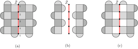
Figure 4: String initialization/measurement method. For initializing the code in an eigenstate of the string operator $\bar{Z}$ shown in a), one can turn off the $X$ stabilizers adjacent to the string and change $Z$ stabilizers next to the string to detach the string and form the code shown in b). Then measure the qubits on the string individually in the $Z$ basis as well as the modified stabilizers for the sake of error correction, which yields the value of $\bar{Z}$. In this step the code effectively looks like (c). After correcting errors, we initialize physical qubits in the $\ket{0}$ state and turn back on all stabilizers in their original form. After $d$ rounds of syndrome measurement and correcting errors, the code is initialized in the $\ket{\bar{0}}$ state.

Suppose for example that we wish to measure the string operator $Z_{1}Z_{2}Z_{3}Z_{4}Z_{5}$, shown in Fig. 4a. We proceed as follows:

1. We turn off every $X$ stabilizer that shares a qubit with the string operator $\bar{Z}$. We also remove every qubit present in $\bar{Z}$ from all $Z$ stabilizers adjacent to it, thus changing the $4$ qubit $Z$ stabilizers adjacent to the string operator to a pair of $2$ qubit $Z$ stabilizers. After making these changes, the code would look like Fig. 4b. Note that practically we have created a new $e$ edge along $\bar{Z}$.

2. We measure qubits $1$-$5$ individually in the $Z$ basis, in addition to performing the stabilizer measurements. We do $d$ rounds of measurements to make the the procedure fault tolerant. Using the value of the individual qubit measurements, along with the measurement outcome of the modified stabilizers, we can recover the value of the original $Z$ stabilizers as well. This allows us to track the errors from before the measurement process began.

3. Finally, we turn on all stabilizers and change all the modified stabilizer operators back to their original form. We need to do $d$ rounds of stabilizer measurements to establish stabilizer values and redefine the code space accordingly.

The measurement of $\bar{Z}$ is obtained by multiplying the measured values for the individual $Z_{i}$ measurements along the string. To make the measurement fault tolerant, it is important to correct any bit flip errors on the $\bar{Z}$ string before using individual measurement outcomes in step 2, and to perform the measurement $d$ times to protect against measurement errors. It is worth noting that one can also measure a ribbon of qubits with thickness $d$ once, instead of measuring a string $d$ times. However, to avoid decreasing the code distance, ribbon measurement requires using larger code patches.

Note that phase flip errors that occur on qubits $1$-$5$ will not change the measurement outcome of $\bar{Z}$ operator.

Measurement in the $\bar{X}$ basis can be done by following similar steps. However, importantly, measurement of $\bar{Y}$ cannot be done in this encoding without introducing additional ingredients, as we describe later.

II.1.3 Quantum computing with planar codes

In order to implement universal fault-tolerant quantum computation, we need to implement a universal gate set fault-tolernatly. For the surface code, a natural choice is the Clifford group, together with the $T$ gate, which is the $\pi/8$ single-qubit phase gate. Here we will briefly review the proposals for implementing logical Clifford gates in the encoding described above. The $T$ gate is then implemented fault-tolerantly using magic state distillation.

The Clifford group is generated by the single-qubit Clifford phase gate, $\bar{S}=\left(\begin{matrix}1&0\\ 0&i\end{matrix}\right)$, $\bar{H}=\frac{1}{\sqrt{2}}\left(\begin{matrix}1&1\\ 1&-1\end{matrix}\right)$, and the two-qubit CNOT gate.

Note that logical $\bar{Z}={\bar{S}}^{2}$ is easy to implement, as one can implement it transversally by applying the single-qubit $Z$ gates on physical qubits along the $\bar{Z}$ string. $\bar{X}=\bar{H}\bar{Z}\bar{H}$ can be applied similarly.

The logical Hadamard gate, $\bar{H}$, is not as straightforward as $\bar{X}$ and $\bar{Z}$. Although applying the Hadamard gate transversally to each individual physical qubit does exchange eigenstates of $\bar{X}$ and $\bar{Z}$, it will also change the boundary conditions, as an $e$ boundary is converted to an $m$ boundary, and vice versa. Therefore, the transversal Hadamard operation does not yield the original code, but rather yields a $\pi/2$ rotated version of it. One then needs to correct the orientation by code deformationDennis et al. (2002); Bombin and Martin-Delgado (2009); Horsman et al. (2012). Code deformation changes the shape of a surface code geometrically by adding physical qubits to the lattice or removing some from it. Adding and removing here does not mean physical changes to the underlying lattice, but it refers to turning on some stabilizers to include some idle physical qubits or turning off some stabilizers to exclude some physical qubits from the code. These additional idle physical qubits add to the spatial overhead required for implementing $\bar{H}$.

The Clifford phase gate, $\bar{S}$ is more complicated in current proposals for the planar code. All current proposals for implementing $\bar{S}$ in planar encoding described above, require state injection and state distillation. There are proposed hybrid schemesBrown et al. (2017) that avoid state distillation for $\bar{S}$ gate which we will mention shortly. In the distillation protocol discussed in Ref. Fowler et al., 2012a, a single round of state distillation takes 7 copies with error probability $p$ and returns one copy with error probability $7p^{3}\ll p$. $k$ rounds of distillation requires $7^{k}$ logical qubits. Therefore the spatial overhead grows exponentially in the number of distillation rounds (See Appendix B). The overhead of performing the Clifford phase gate is thus extremely high. It is worth noting that a modified version of the planar code makes it possible to keep track of single qubit Clifford gates including $\bar{S}$ at the classical level, thus eliminating the need for state distillation by avoiding direct implementation of the $\bar{S}$ gateLitinski and von Oppen (2017a).

The two-qubit logical CNOT gate has been proposed to be implemented as follows. One method is to apply CNOT transversally between every physical qubit in one plane and the corresponding qubit in the other.Dennis et al. (2002) However this operation is non-local if we limit ourselves to a single-layer two-dimensional layout, and thus will not be further considered.

A method for implementing CNOT using local interactions in planar codes uses a method referred to as lattice surgery.Horsman et al. (2012) This method utilizes an extra logical ancilla qubit together with the circuit shown in Fig. 5.Horsman et al. (2012) $M_{O}$ in the circuit indicates measurement of operator $O$.

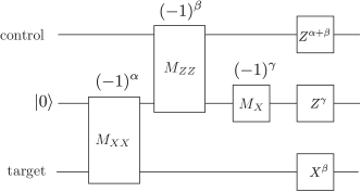
Figure 5: Quantum circuit for CNOT. The number above each measurement represents the outcome of that measurement.

We have already explained how to perform the $M_{X}$ and $M_{Z}$ measurements. What remains is to explain how to perform the joint measurement such as $M_{XX}$ and $M_{ZZ}$ in planar codes. It is important to note that measuring $\bar{Z}_{1}$ and $\bar{Z}_{2}$ separately and then multiplying the result is not equivalent to a $\bar{Z}_{1}\bar{Z}_{2}$ measurement, as the former will project the code into a smaller subspace than intended.

Consider two planar codes next to each other, as in Fig. 6a. Note that the neighboring boundaries are both $m$ boundaries. To measure the two body operator $\bar{Z}_{1}\bar{Z}_{2}$ we use the following steps:

1. We stop measuring the $X_{2}X_{3}$ and $X_{6}X_{7}$ stabilizers and start to measure the combined $X_{2}X_{3}X_{6}X_{7}$ stabilizer. At the same time, we start measuring two new $Z$ stabilizers $Z_{1}Z_{2}Z_{6}Z_{5}$ and $Z_{3}Z_{4}Z_{8}Z_{7}$. This modification effectively merges the two patches together and the code will look like Fig. 6b.

2. We wait for $d$ rounds of stabilizer measurements to establish the values of newly added $Z$ stabilizers.

3. We read the value of $\bar{Z}_{1}\bar{Z}_{2}$ by multiplying the measurement outcomes of newly added $Z$ stabilizers. After that we stop measuring all three shared stabilizers and turn back on $X_{2}X_{3}$ and $X_{6}X_{7}$ stabilizers to detach the codes again.

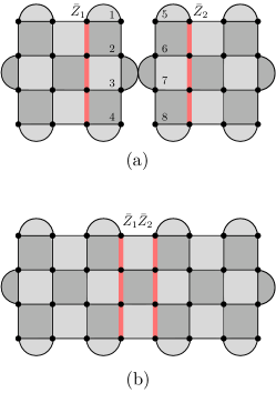
Figure 6: a) Two disjoint planar codes with $\bar{Z}_{i}$ operators shown. b) To measure the parity operator $\bar{Z}_{1}\bar{Z}_{2}$, we turn on all $Z$ stabilizers that are between two patches. We also combine two $2$-qubit $X$ stabilizers at the boundary into one full stabilizer. After $d$ rounds of syndrome measurement and error correction we can find the value of $\bar{Z}_{1}\bar{Z}_{2}$ by multiplying the newly measured $Z$ stabilizers.

If the patches are oriented in such a way that $e$ boundaries are next to each other, we can measure the $\bar{X}_{1}\bar{X}_{2}$ operator by turning on the shared $X$ stabilizers. The procedure is similar to the $M_{ZZ}$ measurement.

Using the joint measurements, the quantum circuit shown in Fig. 5 can be implemented by using the configuration shown in Fig. 7. The logical qubit in the corner is the ancilla qubit, the bottom patch encodes the target qubit and the other one is the control qubit. Note that the patches are oriented in such a way to make the joint measurements in Fig. 5 possible. In the last step, we need to apply single qubit gates based on the outcome of previous measurements as shown in Fig. 5.

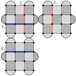
Figure 7: Planar code layout to do the CNOT. The patch in the corner encodes the ancilla qubit, the one in the right is the control qubit and the bottom one is the target qubit.

II.2 Hole encoding

If we start with a planar code and remove some qubits from the bulk, we obtain a hole defect. Fig. 8a shows a hole defect that is created by turning off nine stabilizers. Although the qubits inside the hole are completely detached from the code, they are needed for moving the hole. Each hole introduces new edges and like the outer edges, the boundary of a hole can be either an $e$ edge or $m$ edge. In principle a hole can have mixed boundary conditions, but usually uniform boundaries are used.

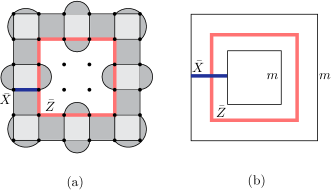
Figure 8: a) Surface code with hole defect in the bulk. Note that both the outer boundary and the hole’s boundary are $m$ boundaries. b) Schematic diagram for the lattice structure shown in (a).

Depending on the boundary type, $e$ or $m$ particles can condense on a hole boundary. This in turn allows one to use hole defects to make new logical operators and thus new logical qubits. The hole defect in Fig. 8, for example, encodes one logical qubit.

In general, $n$ holes of the same boundary type define a $2^{n-1}$ dimensional code subspace. The proposal described in Ref. Fowler et al., 2012a, however, uses a sparse encoding, where each logical qubit is encoded using two holes, as shown in Fig. 9. A logical qubit that is defined using a pair of $e$ boundaries is called a $X$-cut qubit (Fig. 9 left). Likewise, $Z$-cut qubit refers to a logical qubit encoded in a pair of $m$ boundaries (Fig. 9 right).

The sparse encoding allows for implementation of logical gates as described below. Our joint measurement technique, described in the subsequent sections, allows Clifford operations to be implemented using denser encodings, and thus may offer advantages in overhead.

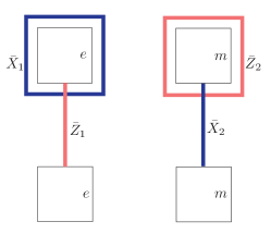
Figure 9: Logical qubits encoded in pairs of hole defects alongside the corresponding logical operators. The outer boundary of the code can be far away and is not shown here.

II.2.1 Quantum computing with hole defects

The measurement and application of the logical $\bar{X}$ and $\bar{Z}$ operators proceeds analogously to the case of the planar encoding. The single qubit Clifford phase gate, $\bar{S}$, is also proposed to be implemented using state injection and state distillation, as in the case of the planar encoding. Similar to the planar code, one can circumvent distillation by using the hybrid schemes Brown et al. (2017) which we will mention shortly.

The single qubit Hadamard gate $\bar{H}$ is performed through a series of code deformationsFowler et al. (2009, 2012a), as follows. Assume we have a pair of $e$ holes encoding our logical qubit. Since, unlike the planar code, there is generally more than one logical qubit encoded in a patch, first we isolate the target logical qubit from the rest by measuring a Pauli $X$ string which encircles the hole pair. As was explained in Sec. II.1.2, this would create an $m$ boundary around the two $e$ holes. By expanding the holes one can turn them into $e$ boundaries of the isolated patch, converting the logical qubit to a planar encoding using boundary defects. The Hadamard gate is then applied as it is in the planar code, described above, and then finally the logical qubit is converted back to the hole encoding and merged into the rest of the code.

The logical CNOT operation is quite different in the hole encoding as compared with the planar encoding. If we have a $Z$-cut qubit and a $X$-cut qubit, one can show that moving a hole of one qubit around a hole of the other, will perform CNOT between the twoRaussendorf et al. (2006); Fowler et al. (2009, 2012a). This process is called hole braiding. However performing CNOT between two qubits with the same type of holes is more complicated, because braiding two holes of the same boundary type is a trivial operation in the code subspace. Instead, in this case one needs extra logical ancilla qubits encoded using holes with the other type of boundary. One can then implement the CNOT gate between two hole defects of the same type through a series of hole braidings and measurements Fowler et al. (2012a). Therefore, to perform a CNOT on two logical qubits requires a total of six holes, if the two logical qubits are both $X$- or $Z$- cut qubits.

II.3 Dislocation encoding

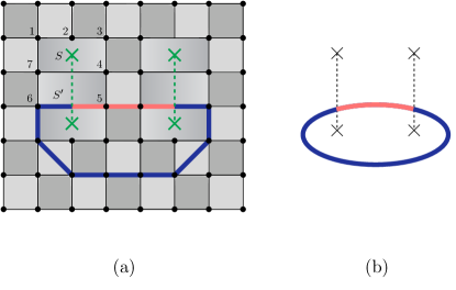
Figure 10: (Color online) (a) A surface code with four twist defects marked by green crosses. The boundary of the surface code is not important and hence has not been shown. Green dashed lines are called dislocation lines. Every twist defect should be connected to another twist defect by a dislocation line. To make a pair of twist defects, we start with a perfect lattice and draw the dislocation line. Then we remove every qubit that lies on the dislocation line. Finally, we combine every two stabilizers that share an edge over the dislocation line into one stabilizer which is given by the product of original stabilizers. Clearly, the contribution of removed qubits have to be omitted. The combined stabilizer is represented by plaquettes with color gradient since they are neither $X$ nor $Z$ stabilizer, but have both operators. It is also possible to create dislocations without removing qubits by having the dislocation lines parallel to the Burgers vectors of the dislocations (not shown here)Bombin (2010); Barkeshli and Qi (2012). (b) Schematic diagram of the surface code shown in (a).

Making holes inside the bulk is not the only way to introduce non-trivial closed loops in surface codes. Twist defects can also be used to induce topological degeneracies and thus to encode logical qubits. Twist defects have been studied from a number of points of view, using topological field theory (see Sec. V of Ref.Barkeshli and Wen, 2010 and Ref.Barkeshli and Qi, 2012; Barkeshli et al., 2013a, b; Teo et al., 2013; Barkeshli et al., 2014), chiral Luttinger liquid theoryBarkeshli and Qi (2012); Barkeshli et al. (2013a, b); Clarke et al. (2013); Cheng (2012); Lindner et al. (2012); Alicea and Fendley (2016), and in lattice models for topological orderBombin (2010); Kitaev and Kong (2012); You and Wen (2012); You et al. (2013).

Fig. 10a illustrates a surface code with four twist defects in the bulk which are marked by green crosses. As is clear from Fig. 10a, the physical qubits on the dislocation lines are removed from the lattice and all pairs of stabilizers that share an edge over the dislocation line are combined into one. The stabilizers located on a twist defect involve five physical qubits, and one of the qubits should be measured in the $Y$ basis. For example, the stabilizer $S$ in Fig. 10a is defined as:

$$S=X_{1}Y_{2}Z_{3}Z_{4}X_{7},$$ (5)

and the stabilizer corresponding to the plaquette just below that is:

$$S^{\prime}=Z_{7}X_{4}X_{5}Z_{6}.$$ (6)

As with hole defects, non-trivial string operators encircling twist defects can be used to define logical qubits. But an important property of dislocation lines is that whenever a string operator passes through them, it changes its type; a Pauli-$Z$ string would change to a Pauli-$X$ string and vice versa. As a result, a closed string operator needs to encircle at least two twist defects. A non-trivial closed string operator is shown as an example at the bottom of Fig. 10a and it includes both Pauli-$X$ and Pauli-$Z$ operators:

$$\bar{Z}=\prod_{i\in\text{light red part}}Z_{i}\prod_{j\in\text{dark blue part}}X_{j}.$$ (7)

One can easily verify that this operator commutes with every stabilizer but is not a product of stabilizers itself. Fig. 10b shows the schematic diagram of the code shown in Fig. 10a.

In general, $n$ pairs of twist defects gives rise to $2^{n-1}$ states. In a dense encoding, therefore, there would be one logical qubit for every pair of twist defects (not counting the first pair). Alternatively, sparser encodings are also possible, using three or four twist defects to encode one logical qubit.

A key feature that distinguishes the dislocation code from planar and hole encodings is that the logical $\bar{Y}$ operator is also given by a simple Pauli string. Therefore the $\bar{Y}$ operator can be straightforwardly measured fault-tolerantly using the same methods for measuring $\bar{X}$ and $\bar{Z}$ operators in the planar and hole encodings. Alternatively, logical qubits can be initialized in the $\bar{Y}$ basis straightforwardly. Fig. 11 shows the logical $\bar{X}$, $\bar{Y}$ and $\bar{Z}$ operators for a logical qubit encoded in three twist defects. It can be shown that any two loop operators that encircle the same set of twist defects are equal to each other up to multiplication by some set of stabilizers and hence represent the same logical operator. For example, both Pauli-$X$ and Pauli-$Z$ strings shown in Fig. 11c are equal to $\bar{Y}$. To prove their equivalence one can use the fact that if a string goes around a single twist twice and closes itself, it acts as the identity on the code subspace (Fig. 12).

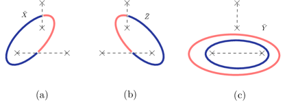
Figure 11: (Color online) Logical operators related to a qubit encoded in three twists. (a) String operator corresponding to $\bar{X}$. It is a mixed Pauli string, with red (light gray) parts corresponding to Pauli $X$ and blue (dark gray) parts corresponding to Pauli $Z$. Note that whenever the string passes through a dislocation line, it changes color. An equivalent string operator for $\bar{X}$ would be the one with red (light gray) and blue (dark gray) interchanged. All that matters is the defects a string enclose. (b) String operator corresponding to $\bar{Z}$. (c) Two equivalent string operators representing $\bar{Y}$.

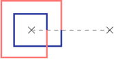
Figure 12: The string that encircles a single twist defect twice and encloses itself can be written as a product of stabilizers and hence acts as the identity operator in the code subspace.

II.3.1 Initialization and measurement

Again, the string initialization and measurement that was described in section II.1.2 can be used here too. It is notable that by using string initialization, one can prepare the $\ket{Y}$ state without using state injection and state distillation procedures.

II.3.2 Quantum Computation by twist defects

The fact that one can measure a logical qubit in the $\bar{Y}$ basis as well as $\bar{X}$ and $\bar{Z}$, allows one to ignore every single-qubit Clifford gate until there is a measurement, and then modify the measurement according to the awaiting gatesHastings and Geller (2014). For example if we want to apply an $S$ gate on a logical qubit and measure it in the $X$ basis, we can ignore the first gate and instead do the measurement in the $S^{\dagger}XS=Y$ basis. This point is explained in more detail in section III.4.

We can also easily implement CNOT using the circuit shown in Fig. 5. Joint measurements in dislocation codes are not really different from single qubit measurements. Suppose we want to measure the $\bar{X}_{1}\bar{X}_{2}$ operator where $\bar{X}_{1}$ is given by a string encircling twists $1$ and $2$ and $\bar{X}_{2}$ encircles twist defects numbered $3$ and $4$. It is easy to see that $\bar{X}_{1}\bar{X}_{2}$ is given by the simple string that encircles all four twist defects $1$ to $4$. We will explain this point further in Sec. IV.2, since joint measurements and twist defects lie at the heart of our method.

II.4 Triangular code

Another important variant of the surface code is called the triangular codeYoder and Kim (2017). Fig. 13 shows a triangular code patch which encodes one logical qubit alongside its schematic diagram. The lattice structure results from flattening a square lattice that resides on three adjacent faces of a cube in three dimensions. There are three boundary defects and one bulk twist defect. Unlike normal twist defects that we mentioned before, the stabilizer $S$ at the position of the bulk twist defect involves four qubits and is given by $S=Y_{1}Z_{2}Z_{3}Z_{4}$. An important distinguishing feature is that in addition to $\bar{X}$ and $\bar{Z}$, the $\bar{Y}$ operator is also given by a simple Pauli string that starts and ends over the edges. As a result, the code can be initialized or be measured in the $\bar{Y}$ basis easily.

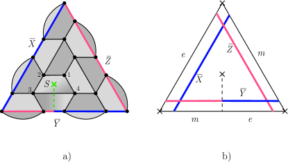
Figure 13: a) A distance $d=5$ triangular code. b) Schematic diagram of the triangular code shown in (a).

A key advantage of the triangular code is that the Clifford phase gate, $\bar{S}$, can be implemented without state distillation, and the general overhead requirements are better than the planar and hole encodings described above.

II.5 Hybrid schemes

Hybrid schemes for encoding logical qubits are also possibleDelfosse et al. (2016); Brown et al. (2017); Litinski and von Oppen (2017a). Mixing two schemes also opens up the possibility of new methods to perform logical operations. For example, by converting boundary defects to bulk twist defects, braiding them and converting them back to the boundary, one can implement the $\bar{S}$ gate in planar codes.Brown et al. (2017) Alternatively, logical qubits in different encodings can be entangled with each other, for example by braiding holes and twist defects.

III Measurement-based protocols for Clifford gates

Here we explain how one can implement all gates in the Clifford group using circuits based on joint measurements. We only discuss the quantum circuits corresponding to the logical gates, regardless of the underlying setup which is used to encode logical qubits. In the subsequent sections, we will show how one can implement these circuits in surface codes, color codes and hyperbolic codes.

In this section all operators are understood to be logical operators, so we will omit the $\bar{\;}$ notation; all qubits are understood to be logical qubits.

III.1 CNOT gate

We have already mentioned the quantum circuit devised to implement CNOT using joint measurements (Fig. 5). It is used in many variants of surface codes as well as color codes to implement the CNOT gateHorsman et al. (2012); Hastings and Geller (2014); Landahl and Ryan-Anderson (2014); Litinski and von Oppen (2017a).

III.2 S gate

The circuit that is shown in Fig. 14 can be used to implement the $S$ gate. Initially, the ancilla qubit is prepared in the $\ket{+}$ state, which is the $+1$ eigenstate of the Pauli $X_{a}$ operator. Next, the two qubit parity operator $ZY_{a}$ is measured, followed by a $Z_{a}$ measurement. The subscript $a$ is used to distinguish the operators associated with the ancilla qubit. The Pauli operators associated with the data qubit will have no subscript.

After the second measurement in Fig. 14, the state of the data qubit is given by:

$$\frac{1-i(-1)^{\alpha+\beta}Z}{\sqrt{2}}|\psi\rangle,$$ (8)

where $(-1)^{\alpha}$ and $(-1)^{\beta}$ are the the results of first and second measurements. Note that the $S$ gate can be written as:

$$S=e^{i\pi/4}\quantity(\frac{1-iZ}{\sqrt{2}}).$$ (9)

Thus, if the outcome of the two measurements have the same sign, the state after the second measurement is, up to an overall phase, $S\ket{\psi}$, and therefore the $S$ gate has been implemented.

On the other hand, if the results of the two measurements are different, the state of the data qubit would be $S^{\dagger}\ket{\psi}$. Since $S=ZS^{\dagger}$, we can recover $S\ket{\psi}$ by applying an additional $Z$ gate to the data qubit.

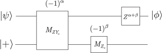
Figure 14: Quantum circuit for S gate. The ancilla is prepared in $\ket{+}=(\ket{0}+\ket{1})/\sqrt{2}$ state. The joint measurement corresponds to measuring the parity of the operator $ZY_{a}$, where the subscript $a$ stand for ancilla qubit and $Z$ is associated with the data qubit. The outcome of each measurement is written above its box.

III.3 SHS gate

We need another independent gate to fully implement the Clifford group. Usually it is the Hadamard gate $H$, but here we choose $SHS$ since it has a simpler circuit. The circuit is shown in Fig. 15. Again, it is easy to check that after the second measurement, the data qubit corresponds to:

$$|\phi\rangle=\frac{1+i(-1)^{\alpha+\beta}X}{\sqrt{2}}|\psi\rangle,$$ (10)

where $(-1)^{\alpha}$ and $(-1)^{\beta}$ are measurement results. Similar to Eqn. 9, we have:

$$SHS=\quantity(\frac{1+iX}{\sqrt{2}}).$$ (11)

So if the results of the two measurements have the same sign, we get the desired state $SHS\ket{\psi}$. Again, if we get different signs, the data qubit would be in the state $S^{\dagger}HS^{\dagger}\ket{\psi}$. We can then recover $SHS\ket{\psi}$ by applying $X$, because $SHS=iXS^{\dagger}HS^{\dagger}$. Hence, at the end of the circuit, we get $\ket{\phi}=SHS\ket{\psi}$.

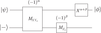
Figure 15: Quantum circuit to implement $SHS$ gate. The ancilla is prepared in the $\ket{-}=(\ket{0}-\ket{1})/\sqrt{2}$ state. The joint measurement corresponds to measurement of the parity of the operator $XY_{a}$, where subscript $a$ stands for ancilla qubit and $X$ is associated with the data qubit. The outcome of each measurement is written above its box.

III.4 Conjugated CNOT circuits

Since single qubit Clifford gates just permute the Pauli matrices (up to a sign), like the $H$ gate that exchanges $X$ and $Z$, it turns out that one can just keep track of them classically instead of actually applying them at the quantum level. One way to see this is to move all single qubit Clifford gates to the end of the circuit and then modify the final measurements accordingly. The price to pay is that for a general quantum circuit, we need to be able to implement CNOT and the $\pi/8$ phase gate $T$ in any Pauli basis. In other words, we need to be able to implement CNOT and $T$ conjugated by any single-qubit Clifford gate.

As an example, consider the quantum circuit shown in Fig. 16a. We use the identity $\text{CNOT}~{}S=S~{}(S^{\dagger}~{}\text{CNOT}~{}S)$ to move the $S$ gate across CNOT. Also since $S^{\dagger}H^{\dagger}\Pi_{\pm,Z}HS=\Pi_{\pm,Y}$ , where $\Pi_{\pm,\sigma}$ denote the projection operator onto the $\pm$ eigenspace of $\sigma$ operator, we can replace the upper $Z$ measurement at the end of the circuit with a $Y$ measurement. So the probabilities for each measurement outcome of this quantum circuit will be equivalent to performing instead $S^{\dagger}~{}\text{CNOT}~{}S$, followed by measurement in a different basis (Fig. 16b). The quantum circuit for $S^{\dagger}~{}\text{CNOT}~{}S$ (Fig. 17) can be derived from the CNOT quantum circuit in Fig. 5.

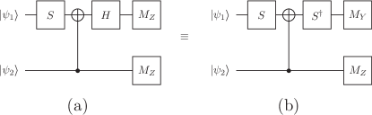
Figure 16: The two quantum circuits in (a) and (b) yield equivalent measurement outcomes, provided the measurements are done in different bases.

Figure 17: $S_{t}^{\dagger}~{}\text{CNOT}~{}S_{t}$ circuit. Here the subscripts $a$, $c$, and $t$ refer to the ancilla, control, and target qubits, respectively.

IV Joint measurement scheme in surface codes

The measurement circuits for the implementation of the $\bar{S}$, $\bar{S}\bar{H}\bar{S}$, and $\overline{\text{CNOT}}$ gates discussed above require the ability to perform joint measurements of operators such as $\bar{Z}\bar{Z}_{a}$, $\bar{X}\bar{X}_{a}$, and $\bar{Z}\bar{Y}_{a}$. Alternatively, if the logical ancilla can be prepared in the $\bar{Y}$ basis, then we only need the joint measurements $\bar{Z}\bar{Z}_{a}$ and $\bar{X}\bar{X}_{a}$.

In this section we will discuss two possible procedures to perform such tasks in surface code. First we explain how one can utilize CAT states to perform the required joint measurements. However, as we will discuss shortly, this method is not practical for large code distances and hence, we introduce the second method which utilizes twist defects to carry out the required measurements.

IV.1 Utilizing CAT states with any encoded ancilla

In many encoding schemes, such as the purely hole or boundary defect based encodings, measuring the logical $\bar{Y}$ operator fault-tolerantly is non-trivial, as the same schemes discussed above for measuring $\bar{X}$ and $\bar{Z}$ do not work. Fig. 18 illustrates the $\bar{Y}$ operator in the hole and boundary defect based encodings, which has support on a graph, as opposed to a string. As such, we refer to it as a graph operator. We see, therefore, that $\bar{Y}$ is a graph operator that contains a $Y$ acting on at least one physical qubit. If we were to directly measure the individual physical qubit operators along the graph, then measuring $Y$ would not give us information about the neighboring $X$ and $Z$ stabilizers, and thus the measurement cannot be made fault-tolerant.

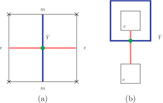
Figure 18: (Color online) a) $\bar{Y}$ operator for a logical qubit encoded in a planar code. b) $\bar{Y}$ operator in hole encoding. The intersection of the red (light gray) and blue (dark gray) strings (marked by the green dot) corresponds to a Pauli-$Y$ operator.

However, we can perform the measurement of $\bar{Y}$ fault-tolerantly with the aid of a CAT state consisting of $k\propto d$ physical ancilla qubits that run along the graph operator, as shown in Fig. 19. As discussed in Ref. Brooks and Preskill, 2013, a CAT state can be prepared with local operations by preparing each qubit in the CAT state in the $\ket{+}$ eigenstate, and then measuring the products $Z_{i}Z_{i+1}$ for nearest neighbor qubits. Armed with the CAT state, we can then measure $\bar{Y}$ using the circuit illustrated in Fig. 20. We refer the reader to Refs. Brooks and Preskill, 2013; Nielsen and Chuang, 2002 for a detailed discussion of the fault-tolerant preparation of CAT states with local operations.

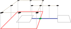
Figure 19: Arrangement of physical ancilla qubits (upper black dots) comprising the CAT state, which is used for fault tolerant measurement of $\bar{Y}$.

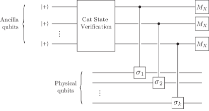
Figure 20: The quantum circuit for preparing a CAT state and measuring a general graph operator of the form $S=\prod_{i=1}^{k}\sigma_{i}$ over physical data qubits. The verification part consists of measuring $Z_{i}Z_{i+1}$ stabilizers $\mathcal{O}(d)$ times and using the result to correct possible bit flip errors.Brooks and Preskill (2013) This would initialize the ancilla qubits into the CAT state. Then, Controlled-Pauli gates are applied between each ancilla qubit and the corresponding data qubit. Afterwards, all ancilla qubits are measured in the $X$ basis. The logical measurement outcome would be equal to the parity of theses individual measurements. The whole measurement procedure is made fault-tolerant by repeating it $\mathcal{O}(d)$ times to obtain a majority vote.

These CAT states can therefore be utilized to either prepare the logical ancilla in an eigenstate of $Y$ by measuring $\bar{Y}_{a}$ or, alternatively, to measure the operator $\bar{Z}\bar{Y}_{a}$, as shown in Fig. 21.

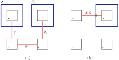
Figure 21: a) A logical data qubit and a logical ancilla qubit encoded in four hole defects. The $\bar{W}$ string does not encode any logical information and can be initialized to $+1$. This idle string would be used to facilitate joint measurements. b) The graph operator corresponding to $\bar{Z}_{1}\bar{Y}_{a}$ can be measured fault tolerantly using CAT states.

We can also apply the above procedure to the case of a $\mathbb{Z}_{2}$ surface code defined on a higher genus surface. On a genus $g$ surface, the $\mathbb{Z}_{2}$ surface code has $4^{g}$ states. The logical Pauli operators for the case of a torus are shown in Fig. 22.

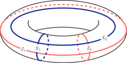
Figure 22: Logical operators that are used to define two logical qubits for a $\mathbb{Z}_{2}$ surface code on a torus.

Using a CAT state, we can then fault-tolerantly measure in the $\bar{Y}$ basis, allowing full implementation of the Clifford group for logical qubits encoded using the genus. For example, on a torus, we have two logical qubits, one of which can be used as a logical ancilla. Utilizing the CAT state for fault-tolerant measurements in the circuits described in Sec. III, we can implement all single-qubit Clifford operations. On higher genus surfaces, we can therefore implement the full Clifford group by using one of the logical qubits as a logical ancilla.

IV.1.1 Application to 3D surface codes

It is interesting to note that this method of performing Clifford gates can be straightforwardly extended to surface codes in higher dimensions as well. In 3 dimensions, the analog of the hole encoding is a sphere encoding, where we consider two far-separated spheres where the $e$ particle is condensed on the surface of the sphere. The logical $\bar{X}$ and $\bar{Z}$ operators are as shown in Fig. 23. The measurement of $\bar{Y}$ could then be achieved with the help of a CAT state consisting of $k$ qubits placed along the support of the $\bar{Y}$ operator.

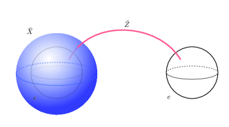
Figure 23: Encoding a logical qubit using two spherical holes in three dimensions. While the logical $Z$ operator is still given by a Pauli-$Z$ string connecting two spheres, the logical $X$ operator is defined as a Pauli-$X$ shell covering the spherical hole.

If $p\,d^{2}\ll 1$, where $p$ is the single qubit error probability, the measurement of graph operators with CAT states require a time overhead $\mathcal{O}(d^{2})$; the preparation of the CAT states requires $\sim d$ steps, while the measurement of $\bar{Y}$ must be performed $\sim d$ times to be fault-tolerant. Furthermore, there is an additional space overhead due to the $\sim d$ physical qubits required for the CAT states. (In 3 dimensions this space overhead is $\mathcal{O}(d^{2})$). However, if $p\,d^{2}$ is of order one or higher, then one needs to repeat the measurement exponentially many times in $d$ to make it fault tolerant. See Appendix A for more detail. Although CAT state measurements can be useful for small codes, it becomes impractical for large code distances. In the next section we introduce another method to perform the required joint measurements to circumvent this problem.

IV.2 Twist defect ancilla

Here we explain how the circuits discussed in Sec. III can be implemented in surface codes without the use of CAT states. We will see for any encoding of logical qubits, as long as we include a logical ancilla encoded with bulk twist defects, we can carry out all of the fault-tolerant measurements required for the circuits in Sec. III .

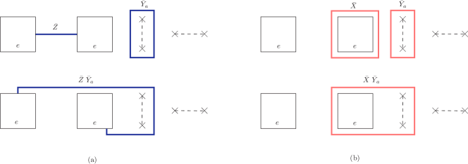
Figure 24: Finding the string corresponding to parity operator measurements in a hole based encoding. Here a pair of $Z$-cut holes are used to encode a logical qubit. There is also an ancilla qubit encoded in four twist defects. Logical operators of the ancilla qubit are specified by subscript $a$. In (a) (top panel), one can see the string operators corresponding to $\bar{Z}$ and $\bar{Y}_{a}$ separately. Both of them are given by a product of Pauli $Z$ operators acting on individual physical qubits. If we want to measure the parity operator $\bar{Z}~{}\bar{Y}_{a}$, we can deform the string corresponding to $\bar{Z}$ in such a way to overlap the left side of the string corresponding to $\bar{Y}_{a}$. Since $\sigma_{Z}^{2}=1$ the overlapping part cancels out, and we would get the connected string shown in the lower panel of (a). In (b) we illustrate the string associated with the parity operator $\bar{X}\bar{Y}_{a}$. Since the logical qubit is encoded in a pair of $Z$-cut holes, the $\bar{X}$ operator is given by a Pauli-$X$ string operator encircling one of the two holes. To do the joint measurement, we use a Pauli-$X$ string encircling the two twists to represent $\bar{Y}_{a}$ shown in (b) up; As we explained, it is equivalent to the Pauli $Z$ string encircling the same twists which we used for the $\bar{Z}~{}\bar{Y}_{a}$ measurement. By deforming the $\bar{X}$ string and making an overlap with the $\bar{Y}_{a}$ string, the shared part cancels out and we get the string shown in the lower panel of (b) for the $\bar{X}~{}\bar{Y}_{a}$ operator.

Here we are going to explain in the context of a simple example how a twist defect ancilla allows the required fault-tolerant joint measurements. Suppose that we have some string operator running through some patch of a surface code, corresponding to a logical operator $O$. It can be a non-trivial loop encircling a hole or some twist defects, or a string that connects two same-type edges in a planar code. Also assume we have a logical qubit encoded in four twist defects in the bulk of the same patch. Imagine we want to measure the parity operator $\bar{O}\,\bar{Y}_{a}$. One can get a simple string corresponding to this operator by deforming the string corresponding to $\bar{O}$ in a way to also encircle the pair of twists that $\bar{Y}_{a}$ encircles. Now, if we measure this new single string operator, using the usual procedures used to measure string operators fault tolerantly, we would get the parity value, without measuring each individual logical operator separately. The same procedure works if one wants to measure other logical parity operators like $\bar{O}\,\bar{X}_{a}$ and $\bar{O}\,\bar{Z}_{a}$; one just needs to deform the string associated with $\bar{O}$ so it encircles the correct pair of twists. The explicit implementation of this procedure when $\bar{O}$ is the logical $X$ or $Z$ operator of a qubit encoded in a pair of $Z$-cut holes is shown in Fig. 24.

Having the tools, implementing each protocol is quite easy. We only explain the $S$ gate implementation in the context of the hole based encoding, but the procedure is essentially the same for other gates (CNOT and $SHS$) in other encoding schemes.

Assume we have a logical qubit $\ket{\psi}$ encoded in a pair of $Z$ cut holes and we want to apply the $S$ gate to it. Assume we have also an ancilla qubit nearby encoded in four twist defects. The following is the step by step description for implementing the $S$ gate:

1. Prepare the ancilla qubit in the $\ket{+}$ logical state (Fig. 25a).

2. Measure the $\bar{Z}\,\bar{Y}_{a}$ string operator shown in Fig. 25b using string measurement method explained in Sec. II.1.2. After reading the measurement result, turn on all the stabilizers and run $d$ rounds of error correction to re-attach the lattice.

3. Measure the $\bar{Z}_{a}$ string shown in Fig. 25c. Again after doing the measurement, turn on all the stabilizers and go through $d$ rounds of error correction.

4. If the results of two measurements had the same sign, the logical qubit has been projected in the $\bar{S}\ket{\psi}$ state and the procedure has been finished. Otherwise, perform a transversal phase flip $\bar{Z}$ gate along the string shown in Fig. 25d to get the desired result.

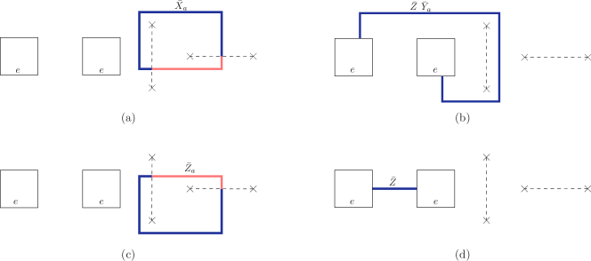
Figure 25: (Color online) $\bar{S}$ gate implementation in hole encoding using a twist defect as ancilla. a) Initialize the ancilla in $\ket{+}$ state, using the string operator shown above. The red (light gray) and blue (dark gray) parts correspond to $X$ and $Z$ Pauli strings respectively. b) Measure parity operator $\bar{Z}~{}\bar{Y}_{a}$ using the Pauli-$Z$ string shown above. After measurement, glue the patch together by doing $d$ rounds of error correction with full stabilizers. c) Measure $\bar{Z}_{a}$ for ancilla qubit, using the string operator shown above and again glue the surface together. d) If the results of two measurements in part b and c had different signs, apply $\bar{Z}$ transversally.

The procedures for implementing $\bar{S}\bar{H}\bar{S}$ and $\overline{\text{CNOT}}$ are quite similar to what is described above. One needs only to choose the right string for the measurement, and re-attach the lattice together after each measurement by going through $d$ rounds of error correction.

Note that the same techniques can also be used for the dense hole encoding, where a logical qubit is defined per each hole instead of two holes. Fig. 26 illustrates the way logical operators are defined in the dense encoding as well as a typical string used for joint measurements. However the dense encodings will not necessarily be advantageous for space overhead, for the following reason.

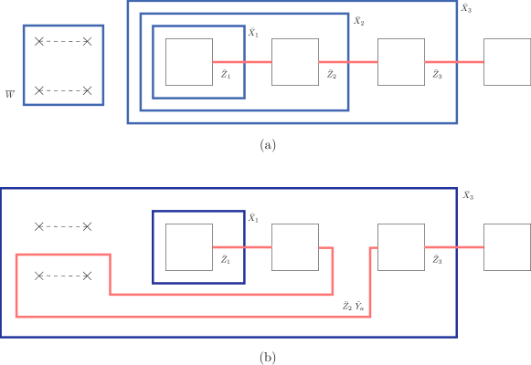
Figure 26: a) One can define $n-1$ logical qubits using $n$ holes in the dense encoding by utilizing the logical operators shown in the figure. Four twist defects on the left are used as an ancilla qubit to implement Clifford gates. The idle string $\bar{W}$ contains no logical information and will be initialized to $+1$. b) Joint measurement is performed by deforming the logical strings to encircle relevant twist defects. Note that the $\bar{W}$ string is used to expand the $\bar{X}_{3}$ operator to protect its information during the $\bar{Z}_{2}~{}\bar{Y}_{a}$ string measurement.

Since the string measurement creates new edges in the system, it can potentially reduce the code distance. One should keep this in mind when performing joint measurements. This issue becomes more pronounced if one needs to measure long string operators, for example in dense encodings (see Fig.  26) , or to perform long range CNOTs even in sparse encodings. In such cases, the string may pass too close to many other logical qubits encoded in the patch.

To avoid this problem during the string measurements, it is always possible to encode the qubits far enough away from each other. However this could be inefficient since usually it increases the spatial overhead considerably. Other workarounds may be possible in certain cases that will result in no or very small increases in spatial overhead. As an example, we will explain how one can address this issue in sparse hole and dislocation encodings.

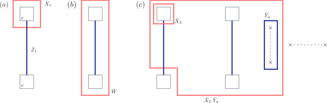
Figure 27: A patch of holes encoding four $X$-cut logical qubits and an ancilla qubit encoded using twist defects. a) Each pair encode a logical qubit with $\bar{Z}$ connecting two holes and $\bar{X}$ encircling the top hole. b) For each pair of holes, the Pauli-$X$ string $\bar{W}$ that encircles both holes in topologically non-trivial but contains no information. We can initialize all such idle strings to $+1$ and use them to extend other strings that need to be measured to maintain the code distance. Note that the Pauli-$Z$ string that encircles the holes can be absorbed into hole boundaries and so is always equal to $+1$. c) How one can utilize idle strings to perform long range joint measurements.

When a hole based encoding is used, typically one places holes on a square lattice with distance $d$ as is depicted in Fig. 27, and each pair stores one qubit of information as usual (Fig. 27a). However, there are still some nontrivial loops, like the string $\bar{W}$ in Fig. 27b, which are not used to encode any information. We call these strings idle strings and utilize these unused degrees of freedom to perform long range string measurements without decreasing the code distance. The idea is that we first initialize all idle strings encircling logical qubits to $+1$ and use them to extend the other strings through the code patch. For example, as is shown in Fig. 27c, to perform the joint measurement $X_{2}Y_{a}$, where $X_{2}$ and $Y_{a}$ are plotted in the figure, one can use the string that also encircles the logical qubit in between, without affecting the measurement result, which in turn helps to keep the code distance $d$. More details can be found in the caption.

A similar idea can be used in dislocation codes. To have a dislocation code with distance $d$ one can arrange twist defects on a rotated square lattice with lattice size $d/\sqrt{2}$ as illustrated in Fig. 28. We can use three twist defects to encode a single logical qubit. In this way for each two logical qubits, there would be a non-trivial idle string that encircles the six twist defects and contains no information. We can initialize these strings to $+1$ and use them to perform long range string measurements without reducing the distance in a similar way to the hole encoding case. As an example, a long range $\bar{X}_{3}~{}\bar{Y}_{a}$ measurement between a logical qubit and an ancilla qubit is shown in Fig. 28. Note that after measuring the shown string the code will divide into two patches, each protected by distance $d$.

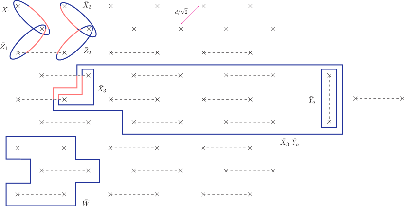
Figure 28: (Color online) Typical arrangement of twist defects on an underlying rotated square lattice with lattice size $d/\sqrt{2}$ which results in a dislocation code with distance $d$. We use $3$ twist defects to encode one logical qubit. The strings that encircles two logical qubits that are encoded in adjacent twist defects, like $\bar{W}$, are non-trivial but contain no information. We initialize all these idle strings to $+1$ to use them for extending measurement strings. Note that the Pauli-$X$ string (red (light gray)) that traces the same path as $\bar{W}$ is equivalent to $\bar{W}$. It is enough to initialize just one of them. c) A long range $\bar{X}_{3}\bar{Y}_{a}$ measurement that maintains the code distance using idle strings. The string passes with at least $d/4$ distance from twist defects. This alongside using idle strings ensures during measurement no short error string could occur.

For the reasons discussed above, dense encodings do not appear to be more advantageous than sparser encodings, in the limit of a large number of logical qubits arranged in a two-dimensional space. On the other hand, for small numbers of logical qubits or logical qubits placed along a line, the dense encodings do have improved spatial overhead than sparser encodings.

IV.2.1 Classical tracking of single qubit gates

As was mentioned in Sec. III.4, instead of applying single qubit gates in a quantum circuit, one can trade CNOT gates in that circuit for conjugated versions of them and modify the final measurements. But this will be useful only if one can implement conjugated versions of CNOT with almost the same number of steps as the CNOT itself. Let us consider the $\bar{S}^{\dagger}~{}\overline{\text{CNOT}}~{}\bar{S}$ circuit (Fig. 17) as an example. The only non-trivial part of that circuit is the $M_{\bar{X}_{a}\bar{Y}_{t}}$ measurement, since this time the $Y$ operator appearing in the operator to be measured is associated with a logical data qubit, whose encoding is arbitrary. For the dislocation code this is clearly not an issueHastings and Geller (2014) because we can measure the logical qubits in any Pauli basis fault tolerantly and hence the same joint measurement techniques described here can be utilized to measure the $\bar{X}_{a}\bar{Y}_{t}$ parity operator.

If the logical qubits are encoded using other types of defects, one needs to find a simple string (as opposed to graph) representation for the parity operator. Remarkably, this can be done in any encoding scheme, as long as there exist ancilla qubits in the twist defect encoding. An example is shown for the case of hole encoding in Fig. 29 where one can find a simple string representation for the parity operator $\bar{X}_{a}\bar{Y}_{t}$. To identify the logical operators in Fig. 29 (a) and (b), we have used the fact that the double loop around a single twist defect is a logical identity (see Fig. 12 ). The $Y$ measurement at the end of the modified quantum circuits can also be done similarly, by initializing the ancilla qubit in $\ket{+}$ state and then measuring the $\bar{X}_{a}\bar{Y}_{t}$ operator.

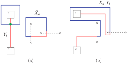
Figure 29: a) $\bar{X}_{a}$ and $\bar{Y}_{t}$ operators. b) $\bar{X}_{a}\bar{Y}_{t}$ operator given by a simple string.

.

V Hyperbolic code

The hyperbolic code is another variant of the surface code that uses different tilings of 2D surfaces to improve the encoding rateBreuckmann and Terhal (2016). Although hyperbolic codes are very efficient for storing information, no procedure is known for fault-tolerant implementation of the Clifford group. Ref. Breuckmann et al., 2017 proposes two possibilities for quantum information processing: (1) to perform Dehn twists, which can be used to either move the qubits around in storage, or to perform a logical CNOT between qubits stored in the same handle, and (2) to use lattice surgery to convert encoded information to a surface code, perform the necessary computations, and convert back to the hyperbolic code.

In this section we demonstrate how our methods can be used to implement fault-tolerantly the full Clifford gate set directly within the hyperbolic code, without moving the information into another quantum code patch.

The hyperbolic code is based on a tiling of a closed surface with regular polygons. A specific tiling is described by a set of two numbers $\{p,q\}$, known as Schläfli symbols, which represents a tiling of the plane with regular $p$-sided polygons such that $q$ of them meet at every vertex. On a Euclidean plane, internal angles of a regular $p$-sided polygon are equal to $(p-2)\pi/p$. On the other hand if $q$ polygons are to meet at a vertex, the internal angles should be equal to $2\pi/q$. Comparing these two, one can see that only tilings with $1/p+1/q=1/2$ can be realized on the Euclidean plane. However, one can use hyperbolic surfaces – surfaces with constant negative curvature – to realize $\{p,q\}$ tilings with $1/p+1/q<1/2$, since the sum of the internal angles of a regular polygon on a hyperbolic plane is less than $(p-2)\pi$. Fig. 30a illustrates the $\{5,4\}$ tiling of the hyperbolic plane.

Given a $\{p,q\}$ tiling, one can define a stabilizer code where physical qubits lie on the edges and each vertex (plaquette) represents a $Z$-type($X$-type) stabilizer. A topologically non-trivial closed hyperbolic surface with $g$ handles has $2g$ non-trivial independent loops which can be used to define $2g$ logical qubits that are stabilized by the code. For large distances and fixed number of physical qubits, hyperbolic codes can encode more logical qubits compared to normal surface codes. However in order to realize such codes in an experimental system that is constrained to the Euclidean plane, non-local interactions are required.

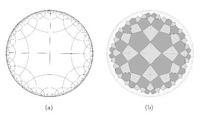
Figure 30: a) $\{5,4\}$ tiling of the hyperbolic plane. b) The rectified tiling r$\{5,4\}$ can be constructed by connecting the midpoints of the edges in the $\{5,4\}$ tiling. The original $\{5,4\}$ tiling is also shown with light solid lines for comparison

If one prefers to work with a form similar to the surface code which was described in Section II, where qubits lie on the lattice sites and all stabilizers are given by plaquette operators, one can use the rectified lattice, denoted by r$\{p,q\}$, which is constructed by connecting the midpoints of the edges in a $\{p,q\}$ lattice(Fig. 30b). The rectified lattice tiles the plane with regular $p$-sided and $q$-sided polygons. In this new form, qubits lie on the vertices and $p$ and $q$ sided plaquettes represent $X$ and $Z$ stabilizers respectively.

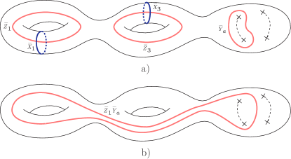
Figure 31: a) Hyperbolic surface with $2$ handles (genus $g=2$) encoding $4$ logical qubits and four twist defects to encode the ancilla qubit. Logical qubits are encoded by using non-trivial loops on the surface. Some logical operators are shown in the figure as examples. The $\bar{X}_{2}$ and $\bar{X}_{4}$ ($\bar{Z}_{2}$ and $\bar{Z}_{4}$) operators are given by Pauli-$X$(Pauli-$Z$) strings that trace out the same loops as $\bar{Z}_{1}$ and $\bar{Z}_{3}$ ($\bar{X}_{1}$ and $\bar{X}_{3}$) operators respectively. b) A sample two qubit parity operator.

The joint measurement circuits for implementing Clifford gates can be used in the hyperbolic codes as well. As in the discussion of the surface code in Sec. IV, we can again consider a set of ancilla qubits that comprise a CAT state in order to help us measure operators that consist of $\bar{Y}_{a}$.

Alternatively, as in the surface code discussion, we do not need any CAT states if we use bulk twist defects to encode a logical ancilla. One can use the original $\{p,q\}$ lattice and create defects in the bulk by following a procedure similar to what was described in Section II.3. However one should be careful not to decrease the code distance and to keep track of what happens to other logical qubits. A more straightforward approach would be to select an arbitrary plaquette, divide it into a $2d\times 2d$ square lattice and create a pair of dislocation lines to encode the logical ancilla qubit. Dividing a plaquette by a square lattice clearly does not change the topology of the surface and keeps the code distance fixed.

Having a logical ancilla qubit encoded with twist defects in hand, performing joint measurements and implementing the quantum circuits described in Section III is straightforward. The single and two qubit parity operators used for Clifford group gates would be given by simple Pauli strings running through the hyperbolic plane (Fig. 31a) . Using the string measurement method, these operators can be measured fault-tolerantly using $d$ rounds of error correction. Fig. 31b shows a typical Pauli string representing a two-qubit parity operator.

There is another variant of the hyperbolic code, the semi-hyperbolic code Breuckmann et al. (2017), where one divides all polygons of a $\{p,q\}$ tilling by a $l\times l$ square lattice. For large $l$ the code would be essentially a normal surface code placed over a topologically non-trivial surface and all efficiency of the hyperbolic construction would be lost. However, it would improve the error threshold of the code Breuckmann et al. (2017). The optimal $l$ should be chosen according to this trade-off. Our joint measurement scheme can be straightforwardly applied to the semi-hyperbolic codes as well, in the same way as the hyperbolic codes.

VI Color code

Color codes are another form of 2D topological codes, with the advantage of higher encoding rates and also allowing for natural transversal logical operations on the qubits. However, color codes usually have smaller error thresholds compared to surface codes. Nevertheless the trade-off between overhead and error thresholds could potentially favor the color codes in future experiments. Although there are already known methods for fault-tolerant quantum computing with color codes Bombin and Martin-Delgado (2006); Fowler (2011); Landahl and Ryan-Anderson (2014), here we point out that implementing the logical Clifford gates using the joint measurement techniques of this paper could have its own advantages. Specifically, performing long-range two-qubit gates are more efficient with our method as compared with the transversal or lattice surgery methods. In contrast to the case of the surface code (without CAT states), our joint measurement protocols can be implemented in the color code in the case where the logical ancilla arises from a hole-based encoding.

The color code can be defined on any three-colorable, three-valent lattice. Qubits lie on the lattice sites and each plaquette corresponds to both $X$ and $Z$ stabilizer operators. The lattice structure ensures that all stabilizers commute with each other. Each stabilizer violation corresponds to a particle. To label the particles we use the color and type of the stabilizer it violates. So, $r_{x}$ denotes a particle detected by a $X$ stabilizer corresponding to a red plaquette. Since we have three different color plaquettes (say red, blue and green), and each plaquette corresponds to two stabilizers, naively there seems to be $6$ independent particles in the theory. However, it can be shown that one can annihilate three particles of the same type and different colors with each otherBombin and Martin-Delgado (2006). Thus, only $4$ out of $6$ are really independent particles. By considering composites of these $4$ types, we find that there are $16$ topologically distinct particles. Indeed, it can be shown that the color code is equivalent (after a finite-depth local unitary transformation) to two copies of the surface code,Kubica et al. (2015) which has a total of $16$ topologically distinct particles.

Just like the surface code, topologically distinct particles always appear in pairs and each pair is connected via Pauli string operators. Since particles carry color, the string operators also would be red, blue or green. For example, a red Pauli-$Z$ string connects two $r_{x}$ particles. Note that a Pauli-$Z$ string violates $X$ stabilizers at its ends but commutes with $Z$ stabilizers.

Similar to the two topologically distinct $e$ and $m$ boundaries in the surface code, the color code can have $6$ topologically distinct types of boundaries, given that it is equivalent to two copies of the surface code (see Ref. Levin, 2013; Barkeshli et al., 2013c, b for a classification of topologically distinct boundary conditions in topological phases). In paticular, the color code can have red, blue and green boundaries where red, blue and green particles can condense.

As in the case of the surface code, logical qubits can be defined through boundary defects, holes, bulk twist defects, or by having non-trivial genus Bridgeman et al. (2017); Fowler (2011); Bombin (2011); Teo et al. (2013).

Holes are created by simply not measuring stabilizers within some region. To create a hole with a red boundary, for example, we consider a closed loop of red string, and stop measuring the stabilizers inside the loop. We also modify the stabilizers on the edge accordingly. Then we have created a hole with a red boundary where red strings can start or end on it without violating stabilizers.

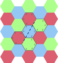
Figure 32: (Color online) Making a twist defect in the color code. To make a twist defect, we first draw the dislocation line (dashed blue line) and remove the qubits which lie on the line. Then we merge pairs of $X$ and $Z$ stabilizers on the sides of the dislocation line into one. Note that in color code each plaquette represents two stabilizers. In this figure half of modified stabilizers are shown. For each stabilizer shown there is another one with $X$ and $Z$ operators exchanged. If the dislocation line passes through a plaquette (like the blue plaquette in the middle), one should merge the $X$ and $Z$ stabilizers corresponding to the same plaquette.

The procedure to create bulk twist defects in the color code is similar to the case of the surface code. One chooses a dislocation line, removes the physical qubits over that line and merges pairs of $X$ and $Z$ stabilizers on either sides into one. Twist defects in surface codes transform $e$ particles to $m$ particles and vice versa. Since color codes have more particles, there are more types of twist defects one can createBarkeshli et al. (2014). In Fig. 32 we have shown one possible example of a pair of twist defects connected to each other with a dislocation line. The one shown in Fig. 32 changes $r_{x}$ to $g_{z}$, $r_{z}$ to $g_{x}$, $b_{x}$ to $b_{z}$ and vice versa, as the particles enircle the twist defect.

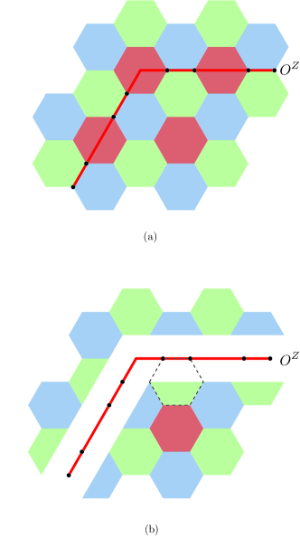
Figure 33: (Color online) String measurement in color codes. a) If we want to measure the red (dark gray) Pauli-$Z$ string operator $O^{Z}$, first we detach the qubits of $O^{Z}$ from neighboring stabilizers and turn off all red (dark gray) stabilizers in its way. b) Then we measure individual qubits in $Z$ basis and multiply the results to find the value of $O^{Z}$. One can correct errors by comparing the value of individual measurements and modified stabilizers with the original value of complete stabilizers. For example, the syndrome of the green stabilizer corresponding to the dashed plaquette before cutting the code, should be equal to the product of measurement outcomes of those two individual qubits and the $4$ qubit stabilizer bellow them.

Based on the underlying encoding scheme, different methods for initialization, measurement and realization of quantum gates can be used. Most of the techniques used in surface codes like lattice surgery and hole braiding have counterparts in color codesLandahl and Ryan-Anderson (2014); Fowler (2011). To measure a string operator, one can practically follow the same procedure used in surface codes. An example is shown in Fig. 33. Let us say we want to measure the red Pauli-$Z$ string operator $O^{Z}$ shown in Fig. 33a. First, we detach from the stabilizers the qubits that lie on $O^{Z}$. This will change some of the green and blue stabilizers from $6$ qubit to $4$ qubit stabilizers. We also need to turn off all red stabilizers which $O^{Z}$ passes through. After the modification, the color code will look like Fig. 33b. Note that this has effectively created a red boundary along the string, where red error strings can start and end without detection. But, just as in the case of the surface code, these undetected errors will not change the value of $O^{Z}$. In the next step, we measure each individual qubit on $O^{Z}$ in the $Z$ basis and also measure all stabilizers. By combining the outcome of individual measurements and modified stabilizers and comparing them with the value of the complete stabilizers, we can detect any error that happens during the measurement process. After correcting the errors, multiplying the outcome of individual measurements would give the value for the measurement outcome of $O^{Z}$.

The joint measurement circuits discussed in this paper for implementing the Clifford group can also be implemented in color codes. If qubits are encoded in a single patch, for example using holes or dislocations, the quantum circuits described in section III can be implemented using a single logical ancilla encoded with twist defects. The rest of the protocol is directly analogous to the case of the surface code.

However, unlike the surface code, in color codes we are not restricted to use twist defects as the logical ancilla to implement the joint measurement method. An interesting feature of color codes is that one can measure not only $X$-type and $Z$-type strings fault tolerantly, but also $Y$-type strings. The reason is that in the color code, in contrast to the surface code, for a given plaquette we measure both $X$ and $Z$ stabilizers and the product of these outcomes gives the value of the corresponding $Y$ stabilizer (we need to multiply it by $(i)^{n}$ where $n$ is the number edges in the plaquette). This feature is a result of the fact that the color code is a CSS code Nielsen and Chuang (2010) constructed from two copies of a single classical code. It is the same property that makes transversal methods natural in this architecture. This in turn enables us to create logical qubits where $\bar{Y}$ is given by a simple Pauli string, without using twist defects.

To implement measurements involving $\bar{Y}$ with a hole encoding, we encode the logical ancilla qubit using three holes associated with different colors, similar to the proposed hole-based encoding in Ref. Fowler, 2011, but with a small modification. Consider the three holes and the graph $G$ that connects them, shown in Fig. 34a. We define $\bar{X}$ as the $G^{X}$ operator, which means the product of Pauli-$X$ operators along the graph, and, similarly, the $\bar{Z}$ as the $G^{Z}$ operator. Since the graph $G$ consists of an odd number of qubits, $G^{X}$ anti-commutes with $G^{Z}$. The advantage of this scheme is that the logical $Y$ operator would be a Pauli-$Y$ graph operator, denoted $G^{Y}$ (in contrast to the proposed method in Ref. Fowler, 2011) and can be measured fault tolerantly.

If we encode the ancilla qubit in the aforementioned three hole structure, no matter how the data qubits are encoded, as long as the logical $X$ and $Z$ operators of the data qubits are given by deformable strings, we can use joint measurement for quantum computation. The idea is similar to what was described in surface codes. For parity measurements, we deform the strings to overlap and measure the resulting string (Fig. 34b). Since the $G$ graph has all three different colors, we can deform it to overlap with any other string operator along a line. Then, the string measurement method can be used to find the parity value fault tolerantly.

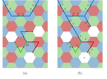
Figure 34: a) Three holes and the $G$ graph that connects them encode the logical ancilla qubit. Blank plaquettes represent holes where we do not measure any stabilizer. $\bar{X}_{a}$, $\bar{Z}_{a}$ and $\bar{Y}_{a}$ are given by $G^{X}$, $G^{Z}$ and $G^{Y}$ respectively. At the top, part of a Pauli string is shown which is a portion of $\bar{X}$ operator related to another logical qubit. b) To measure two qubit parity operator $\bar{Y}_{a}\bar{X}$ one should deform $G$ in such a way to overlap with the string related to $\bar{X}$ and measure the resulting string.

VII Resource analysis

In this section we discuss how our proposed methods inform the design of efficient surface code encoding schemes, and we analyze the associated resource costs and compare them to other proposed methods of quantum computation with the surface code.

In particular, we analyze the resource costs associated with both small and large numbers of logical qubits. For small logical qubits, we propose new surface code schemes for encoding one and two logical data qubits and one logical ancilla qubit, which allow implementation of the full Clifford group using our joint measurement circuits. We compare the resource costs in terms of number of physical qubits required for a given code distance with other proposals presented in the literature. For two logical qubits and being able to perform all Clifford group operations, our proposal is optimal; as such, we expect it could play a useful role in near-term experimental demonstrations of fault-tolerant quantum eror correction.

For large numbers of qubits, we argue that the most optimal method to date for the surface code uses a lattice of dislocations, and we compare the resource costs in terms of number of physical qubits for a given code distance for such an encoding scheme with other proposed methods.

We remark that the hybrid scheme of Ref. Brown et al., 2017 is not included in this comparison. Although the proposed scheme does not use state distillation for implementing Clifford gates and hence is a promising candidate for near term surface code realization, an exact analysis of resource costs for few qubits has not been performed. Ref. Brown et al., 2017 analyzed its asymptotic space overhead scaling for large $d$, although our considerations (not summarized here) of their approach yield different results, so we leave a definitive analysis for future work.

VII.1 Single qubit codes

Let us first consider small codes that admit implementation of all single qubit gates in the Clifford group. In the case of color codes, we only need one logical qubit and we can implement all single qubit Clifford gates transversally. However in some variants of surface codes, we need at least an extra logical ancilla qubit to apply single qubit Clifford gates on logical qubits. The hole-based encoding and lattice surgery methods proposed so far rely on state injection and distillation for implementing the full Clifford group gate set, whereas triangle codes and the surface code with joint measurement, presented in this paper, do not.

A minimal setup that allows one to implement all single qubit Clifford gates using the joint measurement methods of this paper is shown in Fig. 35a. In this configuration, the logical data and ancilla qubits are encoded with both boundary and bulk twist defects. For large $d$, this configuration requires $\sim 4d^{2}$ physical qubits. The explicit $d=3$ lattice construction corresponding to this configuration is shown in Fig. 36.

$d$	$3$	$5$	$7$	$d$
Surface Code (surgery / without distillation)	$27$	$75$	$147$	$\sim 3\,d^{2}$
Surface Code (surgery / one round of distillation)	$55$	$138$	$259$	$\sim 4.75\,d^{2}$
Surface Code (surgery / two rounds of distillation)	$76$	$271$	$343$	$\sim 6.06\,d^{2}$
Surface Code (Triangular)	$37$	$91$	$169$	$\sim 3\,d^{2}$
Surface Code (Joint Measurement)	$40$	$106$	$204$	$\sim 4\,d^{2}$

Table 1: The number of physical qubits needed in order to implement all single qubit Clifford gates in various schemes. We explain the calculation of the overhead costs for the state distillation protocols in Appendix B.

In Table 1, we list the number of physical qubits each design uses to implement all single qubit Clifford gates. The syndrome qubits which are used for the stabilizer measurements are not included in any of the counting. In case of the triangular code, three different schemes have been proposed for implementing single qubit Clifford gatesYoder and Kim (2017); here we used the code conversion (CC) approach for comparison since in this approach single qubit gates are actually implemented rather than kept track of classically. Furthermore, a special design of the triangular code for $d=3$ is proposed in Ref. Yoder and Kim, 2017 which uses only 7 qubits. However, since it cannot be generalized to larger code distances, it is not included in this comparison.

In the case of the surface code proposal using the planar encoding with lattice surgery, we have included the number of physical qubits needed for implementing the full Clifford gate set using zero, one, and two rounds of state distillation. Higher numbers of distillation rounds exponentially decreases the error probability in the purified state. One round of distillation using the Steane codeSteane (1996) uses $7$ instances of noisy logical qubits in the $\ket{Y}$ state to generate a less noisy $\ket{Y}$ state Fowler et al. (2012a). If the input state has error probability $p$, the output state will have $7p^{3}$ probability of having error. So, performing $k$ rounds of state distillation to reduce the error probability to $7^{(3^{k}-1)/2}p^{3^{k}}$, needs $7^{k}$ extra logical ancilla qubits (However they need not be prepared with the full code distance. See Appendix B). Apart from the noisy ancilla qubits initialized in the $\ket{Y}$ state, the distillation process has a number of other overhead costs as well. These include other ancilla qubits initialized in the standard computational basis and additional ancilla qubits required in the planar code layout to perform the logical gate operations with lattice surgery Horsman et al. (2012). The latter for example raises the overhead to $4\times 7^{k}$ logical ancilla qubits. The numbers for one and two rounds of distillation in Table 1 only include the number of physical qubits one needs to prepare the initial noisy $\ket{Y}$ states, thus not including these additional resource costs.

The necessary number of distillation rounds depends on the required accuracy of the purified state. If we assume preparation error and storage error are of the same order, it is reasonable to perform $k\sim\mathcal{O}(\log d)$ rounds of error correction to keep the logical error probability at $\mathcal{O}(p^{d/2})$. This implies that the asymptotic scaling of the space overhead for protocols that require state distillation is $\mathcal{O}(d^{3})$.

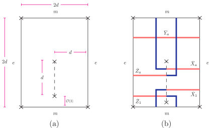
Figure 35: a) The general layout used to encode a logical data qubit and a logical ancilla qubit with distance $d$ that enables one to do all single qubit Clifford gates explicitly. b) The Pauli strings corresponding to logical operators of the main qubit ($\bar{X}_{1}$ and $\bar{Z}_{1}$) and the ancilla qubit ($\bar{X}_{a}$,$\bar{Y}_{a}$ and $\bar{Z}_{a}$).

Figure 36: Distance $d=3$ surface code encoding a logical qubit and an ancilla qubit. Logical operators are defined according to Fig. 35.

VII.2 Two qubit codes

Now we consider small codes that allow full implementation of the Clifford group on two logical qubits, which thus includes the CNOT gate. Almost all proposed designs use the circuit shown in Fig. 5 for performing CNOT, which requires an additional logical ancilla qubit. Two important exceptions are the braiding of bulk defects and transversal methods. Braiding methods need a large space to move defects around and are not suitable for small numbers of qubits. For example the qubit overhead for the double hole implementation scales like $\sim 37/2d^{2}$, which is much worse than other methodsHorsman et al. (2012) and will not be considered here. The transversal methods, in contrast, allow implementation of logical CNOT by independent application of CNOT among physical qubits from different code patches. This uses the minimum number of qubits by eliminating the need for any logical ancilla qubit. However in a two-dimensional single-layer planar geometry, this method relies on long-range interactions when the system scales up to large numbers of qubits and large code distance $d$. We restrict our comparison to methods that utilize only local interactions on a planar geometry in this limit, hence omitting transversal methods from the comparison.

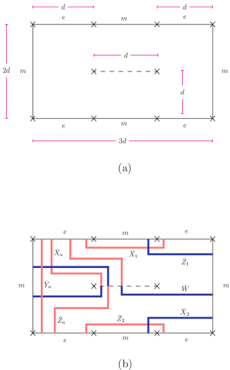
Figure 37: a) The general layout used to encode two logical data qubits and a logical ancilla qubit that enables one to do all Clifford gates explicitly. b) The Pauli strings corresponding to logical operations. The one belonging to the ancilla is specified by $a$ subscript. The $\bar{W}$ string is an idle string that should be initialized to $+1$ so one can use it for fault tolerant joint measurements.

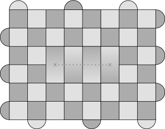
Figure 38: Distance $d=3$ surface code encoding two logical qubit and one ancilla qubit. Logical operators are defined according to Fig. 37.

Fig. 37a is a minimal surface code configuration that can be used to encode two logical data qubits and one logical ancilla qubit, which allows us to implement all Clifford gates using the joint measurement protocols. The ancilla qubit is encoded with twist defects and the logical qubits are encoded using boundary defects. For large $d$, this construction uses $\sim 6d^{2}$ physical qubits. The explicit $d=3$ lattice construction corresponding to this configuration is also shown in Fig. 38.

$d$	$3$	$5$	$7$	$d$
Surface Code (surgery / without distillation)	$36$	$100$	$196$	$\sim 4\,d^{2}$
Surface Code (surgery / one round of distillation)	$64$	$163$	$308$	$\sim 5.75\,d^{2}$
Surface Code (surgery / two rounds of distillation)	$85$	$296$	$392$	$\sim 7.06\,d^{2}$
Surface Code (Triangular)	$74$	$182$	$338$	$\sim 6\,d^{2}$
Surface Code (Joint Measurement)	$60$	$160$	$308$	$\sim 6\,d^{2}$

Table 2: The number of physical qubits to implement all Clifford group gates including CNOT. We use the results of Appendix B for the state distillation overhead costs.

Table 2 lists the number of physical qubits that various methods use to implement the full Clifford group. Again, the numbers for surface code with distillation reflect only the number of qubits used in encoding noisy $\ket{Y}$ states in the lowest layer of distillation. As one can see, the joint measurement method of this paper uses the minimum number of physical qubits among other surface code variants, but scales the same as the triangular code for large $d$.

VII.3 Many qubit codes

The two previous sections discussed encodings for one or two logical qubits (and a logical ancilla). If we consider large scale quantum computing with more than just three total qubits, there are more clear advantages for using the proposed joint measurement design for gates.

First, the joint measurement protocol naturally allows CNOT gates between two logical qubits that are arbitrarily far apart from each other. By encoding all logical qubits within the same patch of surface code (e.g. using bulk twist defects or holes), we can measure arbitrarily long strings with no additional space-time overhead. This means that even the logical ancilla qubit in the CNOT circuit does not need to be physically near the control and target logical qubits. On the other hand, the lattice surgery based methods (which is used by both planar and triangular surface codes) only allow operations between adjacent patches of the code. Thus, a CNOT gate between far-separated qubits requires bringing the two patches near each other first. Apart from the time overhead this operation imposes, it necessitates sufficient blank patches between data qubits, which results in increased space overhead; One can show that for a typical arrangement of square patches of planar codes, only a quarter of patches can be used for storing data and other patches should be reserved as blank spaces to be used for moving data patches aroundHorsman et al. (2012).

A natural question now is which particular type of encoding is most efficient, in the limit of large numbers of logical qubits, for minimizing the number of physical qubits for a given code distance. We find that the optimal encoding is with a lattice of bulk twist defects (dislocations). Such a dislocation code was discussed in Ref. Hastings and Geller, 2014; however our proposal and results for resource estimates differ somewhat from those reported previously. Specifically, we consider an arrangement of twist defects as shown in Fig. 28. The twist defects are placed on a rotated square lattice with lattice constant $d/\sqrt{2}$, in contrast to the square lattice with lattice constant $d/2$ that was proposed in Ref. Hastings and Geller, 2014. We require this modification to protect the code from Pauli-$Y$ error strings that can start and end on the twist defects.

Furthermore, since long-range CNOT gates require measuring long-range string operators, it is important to keep the code distance $d$ throughout the measurement process. To ensure this, we initialize the idle strings (like $\bar{W}$ in Fig. 28) to $+1$ and by utilizing them, we thread the strings through the available space between the defects in such a way that every twist defect is at least distance $d/4$ apart from the measured string, as is shown in Fig. 28. This ensures that no short error string could happen while measuring the strings. More details can be found in the caption. By adding one ancilla qubit to the patch and using the joint measurement method, one can apply all Clifford gates fault tolerantly.

In Table 3, we have listed encoding rates for various schemes for comparison. For the lattice surgery method on planar codes, the $(7/4)^{k}~{}d^{2}$ term arises from the additional logical ancilla qubits needed for state distillation(See Appendix B). As was explained in Sec. VII.1, one needs $\mathcal{O}(\log d)$ rounds of state distillation to obtain $\sim p^{d/2}$ logical error probability. This in turn means the additional cost due to state distillation grows like $d^{3}$ and dominates the resource usage. In the case of the triangular code, Ref. Yoder and Kim, 2017 proposed several protocols; in Table 3, we quoted the encoding rate when one keeps track of single qubit gates at the classical level instead of applying them directly on the quantum code (referred to as the basis-state conversion (BC) scheme). We see that the joint measurement method with a lattice of bulk twist defects performs better than both of these.

We note that the direct comparison of different encoding schemes summarized in Table 3 involves some subtleties as the different schemes also have various relative advantages. For example, the joint measurement estimate assumes a single logical ancilla for an arbitrary number of logical gates, while the estimates for the other schemes assume a number of logical ancillas that grows with the number of logical qubits. On the other hand, the joint measurement scheme allows arbitrarily long-range CNOT gates, while the other two schemes do not. Furthermore, we note that Ref. Litinski and von Oppen, 2017a has proposed an alternative patch-based scheme that allows classical tracking of the single-qubit Clifford gates; however a direct comparison with that proposal is more complicated, as it allows for many possible distinct designs.

Scheme	$N_{phys}/N_{L}$
Surface Code (Surgery / $k$ rounds of distillation)	$4(1+\quantity(\frac{7}{4})^{k})\,d^{2}\sim d^{3}$
Surface Code (Triangular)	$9/4\,d^{2}$
Surface Code (Joint Measurement)	$3/2\,d^{2}$

Table 3: Asymptotic encoding ratio for large number of logical qubits, while being able to implement all Clifford gates.

One can improve these scaling relations for the encoding rate by using non-local interactions and thus implementing hyperbolic codes. As discussed in Sec. V, our joint measurement proposal is so far the only proposed method to implement the full Clifford group in hyperbolic codes.

VIII Conclusion

We have shown that every encoding scheme in the surface code admits a fault-tolerant implementation of the full Clifford gate set, without the need for state distillation or conversion between different types of encodings as required in a number of previous proposals. If the logical ancilla is encoded using boundary defects, holes, or through non-trivial genus, then a CAT state can be used to implement the required topological charge measurements. On the other hand, if the logical ancilla is encoded with bulk twist defects, then the CAT state is not necessary, and the full Clifford gate set can be directly implemented. We have further shown how these methods allow implementations of the Clifford group in the 3D surface code with a sphere encoding. We also used these methods to provide the first proposals for implementing the full Clifford group in hyperbolic codes, and a new scheme for implementing them in the color code, which allows arbitrarily long-range CNOT gates.

Our joint measurement proposal also informs efficient surface code designs. In particular, we have proposed designs for one and two logical qubits and one logical ancilla qubit, which admit fault-tolerant implementation of the full Clifford group. In the case of two logical qubits and one ancilla, our proposal is an improvement over all previous proposals in terms of number of physical qubits required for a given code distance $d$. As such, they may be of use for near-term experiments to demonstrate fault-tolerant implementation of logical gates.

For large numbers of logical qubits, we have found that a lattice of twist defects (the dislocation code) is optimal in terms of spatial overhead. While such a code was studied in Ref. Hastings and Geller, 2014, our analysis of the resource overhead and scheme for performing long-range CNOT gates is distinct.

Ultimately, for quantum computing applications, an added advantage of the dislocation code, as pointed out in Ref. Hastings and Geller, 2014, is that the single-qubit Clifford gates add nothing to the time overhead, as they can effectively be absorbed into the CNOT gates by picking different strings to measure along. Similar advantages exist in the triangular codeYoder and Kim (2017) and certain patch-based proposals, as discussed in Ref. Litinski and von Oppen, 2017a. We have shown that similar advantages exist for our protocols as well and thus exist for any encoding scheme, as long as logical ancilla qubits are implemented in the surface code with twist defects. In contrast, the single qubit Clifford gates will need to be performed for the proposals of Ref. Fowler et al., 2012a; Horsman et al., 2012. Nevertheless, it presumably would be useful to actually implement single-qubit Clifford gates in small near-term quantum computers in order to demonstrate experimentally the possibility of implementing fault-tolerant logical gates.

IX Acknowledgment

We thank Isaac Kim for helpful discussions. This work is supported by NSF CAREER (DMR-1753240) and JQI-PFC-UMD.

Appendix A Time overhead estimate for CAT state measurements

Here we discuss the time overhead for utilizing CAT states for performing logical measurements. In order to measure a string operator $S=\Pi_{i=1}^{d}\sigma_{i}$ using cat states, first we prepare the measurement qubits in the $\ket{+}^{d}$ state and then measure $Z_{i}Z_{i+1}$ stabilizers for $d$ rounds. Next we perform controlled $\sigma_{i}$ gates between the measurement qubits and corresponding data qubits and at last we measure measurement qubits in $X_{i}$ basis and infer the measurement results form the overall parity of outcome.

Bit flip errors are generally taken care of by the syndrome measurements so here, we concentrate on the phase flip errors. Since phase flip errors cannot be detected by stabilizer measurements, we need to repeat the measurement many times and decide on the value of measurement by taking a majority vote. Here we provide an estimate on the number of measurements $r$ one needs to achieve fault tolerance.

We only consider phase flip errors that occur during storage intervals. It is reasonable to expect that including other types of errors will not change the answer significantly.

We have $d$ measurement qubits. During preparation of the CAT state, we perform $d$ rounds of stabilizer measurements. So during preparation, we consider $d^{2}$ space-time points where phase flip errors can happen. Applying controlled $\sigma_{i}$ gates can be done simultaneously in one step, therefore it adds $d$ places to the potential locations for phase flip errors. Thus there are $\mathcal{O}(d^{2})$ spots where phase flip errors can happen during a single round of CAT state measurement. For simplicity we take this number to be $d^{2}$.

Let’s say the probability of a phase flip error affecting a single qubit during a single time step is given by $p$. Note that if an even number of such errors occur during a round of measurement, we still get the right answer. To find the probability of this happening, we use the following recursive expression for having even number of errors in the first $n$ locations,

$$P_{n+1}=P_{n}(1-p)+(1-P_{n})p.$$ (12)

This difference equation can be solved easily to get,

$$q\equiv P_{d^{2}}=\frac{1}{2}+\frac{1}{2}(1-2p)^{d^{2}}.$$ (13)

Although this result is exact, we are only interested in the $p\ll 1$ limit:

$$q=\frac{1}{2}+\frac{1}{2}e^{-2p\,d^{2}}$$ (14)

$q$ gives the probability of getting the right answer after a single measurement. If $pd^{2}\ll 1$, then we have,

$$q=1-pd^{2},$$ (15)

and therefore to reduce the probability of failure to $p^{d/2}$, it suffices to repeat the measurement $\mathcal{O}(d)$ times,

$$r\sim\mathcal{O}(d),\qquad pd^{2}\ll 1.$$ (16)

However, if $pd^{2}\gg 1$, $q$ will be exponentially close to $1/2$ and we need a huge number of measurements to make sure the majority vote gives the right answer.

To find out how many times we need to repeat the measurement, we can use the central limit theorem. First we define the following statistical variable:

$$X=\begin{cases}1&\text{with probability }q\\ 0&\text{with probability }1-q\end{cases}$$ (17)

basically $X$ would be $1$ when we get the right answer and $0$ otherwise. Note that the mean and variance of $X$ is given by $\expectationvalue{X}=q$ and $\sigma^{2}_{X}=q(1-q)$ respectively. If we repeat the measurements $r$ times, the quantity which we are interested in is given by,

$$S=\frac{\sum_{i=1}^{r}X_{i}}{r}$$ (18)

If $S>1/2$ the majority vote gives the right answer and if $S<1/2$ we get the wrong answer. It is well known that for $r\gg 1$, the distribution function of $S$ can be well approximated by a normal distribution around $\mu_{S}=\expectationvalue{X_{i}}$ with standard deviation $\sigma_{S}=\frac{\sigma_{X}}{\sqrt{r}}$.

Using this distribution, it is easy to see that the probability of getting $S>1/2$ is given by:

$$P_{\text{failure}}=\frac{1}{2}\,\operatorname{erfc}(e^{-2pd^{2}}\sqrt{\frac{r}{2}})$$ (19)

where $\operatorname{erfc}(x)$ is the complementary error function given by,

$$\operatorname{erfc}(x)=\frac{2}{\sqrt{\pi}}\int_{x}^{\infty}e^{-t^{2}}\differential t.$$ (20)

For large $x$s, $\operatorname{erfc}(x)$ can be approximated by,

$$\operatorname{erfc}(x)=\frac{e^{-x^{2}}}{\sqrt{\pi}x}(1+\mathcal{O}(x^{-1}))$$ (21)

using this asymptotic form alongside Eq.(19), one can see that for $pd^{2}\ll 1$, to get $P_{\text{failure}}\sim p^{d}$, we need to repeat the measurement exponentially many times,

$$r\sim\mathcal{O}(e^{\alpha d^{2}}),\qquad pd^{2}\gg 1.$$ (22)

We remark that although this will make the method fault tolerant, it renders this method quite unpractical in this regime.

Appendix B Space overhead for state distillation

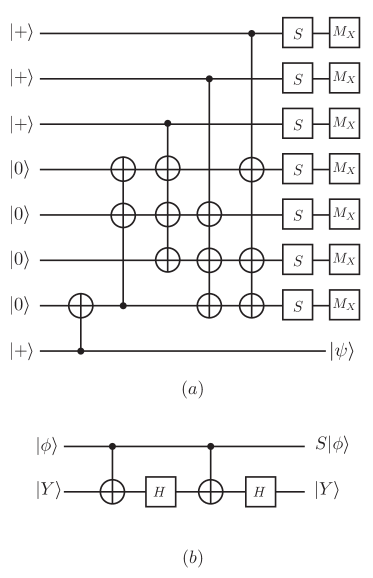
Figure 39: a)The quantum circuit used to purify $\ket{Y}$ states. b) The quantum circuit used to implement $S$ gates in the distillation circuit which uses an ancilla prepared in $\ket{Y}$ state. The ancilla is either initialized by state injection technique(in the lowest layer of distillation) or is the purified output of previous rounds of distillation.

In this section we briefly estimate the space overhead incurred by state distillation and thus explain how the numbers in Tables 1 and 2 were calculated.

The distillation circuit for logical $\ket{Y}$ state based on the Steane codeSteane (1996) is illustrated in Fig.39aFowler et al. (2012a). We will not cover the details of this circuit here; the interested reader can consult Refs.Fowler et al., 2012a; Steane, 1996 for a through explanation. Basically, in each round of distillation seven noisy $\ket{Y}$ states are input into the circuit through the $S$ gates (as shown in Fig.39bFowler et al. (2012a)) and after the final measurements, with some finite fixed probability, $\ket{\psi_{L}}$ will collapse to a purified version of $\ket{Y}$ (or $\bar{Z}\ket{Y}$ which can be corrected easily).

For $k$ rounds of distillation, one starts with $7^{k}$ noisy logical qubits prepared in the $\ket{Y}$ state using state injection. After the first round of distillation, $7^{k-1}$ purified states would be produced, which then will be used for the next round of distillation. Applying distillation $k-1$ more times by using the output of previous rounds as the input to the next round will result in a single distilled $\ket{Y}$ state with error probability $\sim p^{3^{k}}$. A lower bound for the space overhead of distillation can be obtained by only counting the number of qubits used in preparing those $7^{k}$ initial $\ket{Y}$ states.

When performing many layers of distillation, there is no point in using logical qubits with the full distance $d$ in every layer, as required in the final layer of distillation, since the input states are noisy anyways. Instead one can, for example, halve the code distance at each lower level to reduce the space overhead. Considering this, initial $\ket{Y}$ states can be prepared using surface codes of distance $\frac{d}{2^{k}}$. If $\frac{d}{2^{k}}<1$ then there is no need to encode the initial states into the surface code by state injection; one can just start with $7^{k}$ physical qubits initialized in $\ket{Y}$ state.

Therefore in this scheme we need a total of

$$N=7^{k}\times\Big{\lceil}\frac{d}{2^{k}}\Big{\rceil}^{2}$$ (23)

physical qubits just to encode the noisy $\ket{Y}$ states in the lowest level. Note that this is a lower bound on the overhead incurred by state distillation, since we have not included other ancilla qubits which are used in distillation circuit. The numbers in Tables 1 and 2 for surface code with distillation are calculated by adding this overhead to basic resource costs. We also note that it may be possible to further optimize the state distillation protocol and thus further reduce the constant factors involved in the space overhead; a complete analysis of such an optimization is beyond the scope of this paper.

References

- Terhal (2015) B. M. Terhal, Rev. Mod. Phys. 87, 307 (2015).
- Campbell et al. (2017) E. T. Campbell, B. M. Terhal, and C. Vuillot, Nature 549, 172 (2017).
- Fowler (2013a) A. G. Fowler, Phys. Rev. A 87, 040301 (2013a).
- Kitaev (2003) A. Kitaev, Annals Phys. 303, 2 (2003), arXiv:quant-ph/9707021 .
- Wang (2008) Z. Wang, Topological Quantum Computation (American Mathematical Society, 2008).
- Nayak et al. (2008) C. Nayak, S. H. Simon, A. Stern, M. Freedman, and S. D. Sarma, Rev. Mod. Phys. 80, 1083 (2008).
- Bravyi et al. (2010) S. Bravyi, D. Poulin, and B. Terhal, Physical review letters 104, 050503 (2010).
- Bravyi and Kitaev (1998) S. Bravyi and A. Y. Kitaev, (1998), arXiv:quant-ph/9811052 .
- Dennis et al. (2002) E. Dennis, A. Kitaev, A. Landahl, and J. Preskill, Journal of Mathematical Physics 43, 4452 (2002), https://doi.org/10.1063/1.1499754 .
- Fowler et al. (2012a) A. G. Fowler, M. Mariantoni, J. M. Martinis, and A. N. Cleland, Phys. Rev. A 86, 032324 (2012a).
- Stephens (2014a) A. M. Stephens, Physical Review A 89, 022321 (2014a).
- Bombin and Martin-Delgado (2006) H. Bombin and M. A. Martin-Delgado, Phys. Rev. Lett. 97, 180501 (2006).
- Freedman et al. (2002) M. H. Freedman, D. A. Meyer, and F. Luo, in Mathematics of Quantum Computation (Chapman and Hall, London, U.K., 2002) pp. 287–320.
- Breuckmann and Terhal (2016) N. P. Breuckmann and B. M. Terhal, IEEE Transactions on Information Theory 62, 3731 (2016).
- Breuckmann et al. (2017) N. P. Breuckmann, C. Vuillot, E. Campbell, A. Krishna, and B. M. Terhal, Quantum Science and Technology 2, 035007 (2017).
- Kubica et al. (2015) A. Kubica, B. Yoshida, and F. Pastawski, New Journal of Physics 17, 083026 (2015).
- Stephens (2014b) A. M. Stephens, arXiv preprint arXiv:1402.3037 (2014b).
- Landahl and Ryan-Anderson (2014) A. J. Landahl and C. Ryan-Anderson, (2014), arXiv:1407.5103 .
- Horsman et al. (2012) C. Horsman, A. G. Fowler, S. Devitt, and R. V. Meter, New Journal of Physics 14, 123011 (2012).
- Hastings and Geller (2014) M. B. Hastings and A. Geller, (2014), arXiv:1408.3379 .
- Litinski and von Oppen (2017a) D. Litinski and F. von Oppen, (2017a), arXiv:1709.02318 .
- Yoder and Kim (2017) T. J. Yoder and I. H. Kim, Quantum 1, 2 (2017).
- Brown et al. (2017) B. J. Brown, K. Laubscher, M. S. Kesselring, and J. R. Wootton, Phys. Rev. X 7, 021029 (2017).
- Bonderson et al. (2009) P. Bonderson, M. Freedman, and C. Nayak, Annals of Physics 324, 787 (2009).
- Barkeshli and Freedman (2016) M. Barkeshli and M. Freedman, Phys. Rev. B 94, 165108 (2016).
- Cong et al. (2016) I. Cong, M. Cheng, and Z. Wang, (2016), arXiv:1609.02037 .
- Litinski and von Oppen (2017b) D. Litinski and F. von Oppen, (2017b), arXiv:1708.05012 .
- Freedman and Meyer (2001) M. H. Freedman and D. A. Meyer, Foundations of Computational Mathematics 1, 325 (2001).
- Edmonds (1965a) J. Edmonds, Canadian Journal of mathematics 17, 449 (1965a).
- Edmonds (1965b) J. Edmonds, Journal of Research of the National Bureau of Standards B 69, 55 (1965b).
- Heim et al. (2016) B. Heim, K. M. Svore, and M. B. Hastings, arXiv preprint arXiv:1609.06373 (2016).
- Baireuther et al. (2018) P. Baireuther, M. Caio, B. Criger, C. Beenakker, and T. O’Brien, arXiv preprint arXiv:1804.02926 (2018).
- Duclos-Cianci and Poulin (2010) G. Duclos-Cianci and D. Poulin, Physical review letters 104, 050504 (2010).
- Duclos-Cianci and Poulin (2013) G. Duclos-Cianci and D. Poulin, arXiv preprint arXiv:1304.6100 (2013).
- Fowler (2013b) A. G. Fowler, arXiv preprint arXiv:1307.1740 (2013b).
- Wang et al. (2003) C. Wang, J. Harrington, and J. Preskill, Annals of Physics 303, 31 (2003).
- Fowler (2012) A. G. Fowler, Phys. Rev. Lett. 109, 180502 (2012).
- Watson and Barrett (2014) F. H. Watson and S. D. Barrett, New Journal of Physics 16, 093045 (2014).
- Fowler et al. (2012b) A. G. Fowler, A. C. Whiteside, A. L. McInnes, and A. Rabbani, Physical Review X 2, 041003 (2012b).
- Raussendorf et al. (2007) R. Raussendorf, J. Harrington, and K. Goyal, New Journal of Physics 9, 199 (2007).
- Fowler et al. (2012c) A. G. Fowler, A. C. Whiteside, and L. C. Hollenberg, Physical review letters 108, 180501 (2012c).
- Bombin and Martin-Delgado (2009) H. Bombin and M. Martin-Delgado, Journal of Physics A: Mathematical and Theoretical 42, 095302 (2009).
- Fowler et al. (2009) A. G. Fowler, A. M. Stephens, and P. Groszkowski, Physical Review A 80, 052312 (2009).
- Raussendorf et al. (2006) R. Raussendorf, J. Harrington, and K. Goyal, Annals of Physics 321, 2242 (2006).
- Bombin (2010) H. Bombin, Phys. Rev. Lett. 105, 030403 (2010), arXiv:1004.1838 .
- Barkeshli and Qi (2012) M. Barkeshli and X.-L. Qi, Phys. Rev. X 2, 031013 (2012), arXiv:1112.3311 .
- Barkeshli and Wen (2010) M. Barkeshli and X.-G. Wen, Phys. Rev. B 81, 045323 (2010), see Sec. V. A, arXiv:0909.4882 .
- Barkeshli et al. (2013a) M. Barkeshli, C.-M. Jian, and X.-L. Qi, Phys. Rev. B 87, 045130 (2013a), arXiv:1208.4834 .
- Barkeshli et al. (2013b) M. Barkeshli, C.-M. Jian, and X.-L. Qi, Phys. Rev. B 88, 235103 (2013b).
- Teo et al. (2013) J. C. Teo, A. Roy, and X. Chen, (2013), arXiv:1306.1538 .
- Barkeshli et al. (2014) M. Barkeshli, P. Bonderson, M. Cheng, and Z. Wang, (2014), arXiv:1410.4540 .
- Clarke et al. (2013) D. J. Clarke, J. Alicea, and K. Shtengel, Nature Comm. 4, 1348 (2013), arXiv:1204.5479 .
- Cheng (2012) M. Cheng, Phys. Rev. B 86, 195126 (2012), arXiv:1204.6084 .
- Lindner et al. (2012) N. H. Lindner, E. Berg, G. Refael, and A. Stern, Phys. Rev. X 2, 041002 (2012), arXiv:1204.5733 .
- Alicea and Fendley (2016) J. Alicea and P. Fendley, Annual Review of Condensed Matter Physics 7, 119 (2016), https://doi.org/10.1146/annurev-conmatphys-031115-011336 .
- Kitaev and Kong (2012) A. Kitaev and L. Kong, Comm. Math. Phys. 313, 351 (2012).
- You and Wen (2012) Y.-Z. You and X.-G. Wen, Phys. Rev. B 86, 161107 (2012).
- You et al. (2013) Y.-Z. You, C.-M. Jian, and X.-G. Wen, Phys. Rev. B 87, 045106 (2013).
- Note (1) Fig. 10 illustrates dislocation lines that run perpendicularly to their Burgers vectors. It is also possible to consider a lattice geometry with dislocation lines parallel to the Burgers vectors, so that qubits do not need to be removed to create a dislocation.
- Delfosse et al. (2016) N. Delfosse, P. Iyer, and D. Poulin, (2016), arXiv:1606.07116 .
- Brooks and Preskill (2013) P. Brooks and J. Preskill, Physical Review A 87, 032310 (2013).
- Nielsen and Chuang (2002) M. A. Nielsen and I. Chuang, “Quantum computation and quantum information,” (2002), see Section 10.6.3.
- Fowler (2011) A. G. Fowler, Phys. Rev. A 83, 042310 (2011).
- Levin (2013) M. Levin, Phys. Rev. X 3, 021009 (2013).
- Barkeshli et al. (2013c) M. Barkeshli, C.-M. Jian, and X.-L. Qi, Phys. Rev. B 88, 241103(R) (2013c).
- Bridgeman et al. (2017) J. C. Bridgeman, S. D. Bartlett, and A. C. Doherty, arXiv preprint arXiv:1708.08930 (2017).
- Bombin (2011) H. Bombin, New Journal of Physics 13, 043005 (2011).
- Nielsen and Chuang (2010) M. A. Nielsen and I. L. Chuang, “Quantum computation and information theory,” (2010).
- Steane (1996) A. Steane, in Proceedings of the Royal Society of London A: Mathematical, Physical and Engineering Sciences, Vol. 452 (The Royal Society, 1996) pp. 2551–2577.