Vibrational Satellites of C2S, C3S, and C4S:                                                                                                               Microwave Spectral Taxonomy as a Stepping Stone to the Millimeter-Wave Band${}^{\dagger}$
	Brett A. McGuire,${}^{a,b,{\ddagger}}$ Marie-Aline Martin-Drumel,${}^{b,\S}$ Kin Long Kelvin Lee,${}^{b}$ John F. Stanton,${}^{c}$ Carl A. Gottlieb,${}^{b}$ and Michael C. McCarthy${}^{\ast,b,d}$
	We present a microwave spectral taxonomy study of several hydrocarbon/CS2 discharge mixtures in which more than 60 distinct chemical species, their more abundant isotopic species, and/or their vibrationally excited states were detected using chirped-pulse and cavity Fourier-transform microwave spectroscopies. Taken together, in excess of 85 unique variants were detected, including several new isotopic species and more than 25 new vibrationally excited states of C2S, C3S, and C4S, which have been assigned on the basis of published vibration-rotation interaction constants for C3S, or newly calculated ones for C2S and C4S. On the basis of these precise, low-frequency measurements, several vibrationally exited states of C2S and C3S were subsequently identified in archival millimeter-wave data in the 253–280 GHz frequency range, ultimately providing highly accurate catalogs for astronomical searches. As part of this work, formation pathways of the two smaller carbon-sulfur chains were investigated using ${}^{13}$C isotopic spectroscopy, as was their vibrational excitation. The present study illustrates the utility of microwave spectral taxonomy as a tool for complex mixture analysis, and as a powerful and convenient ‘stepping stone’ to higher frequency measurements in the millimeter and submillimeter bands.

1 Introduction

Quantitative chemical analysis of complex mixtures is of interest to a broad range of fields ranging from atmospheric and combustion science,¹ to the food industry,² and astrochemistry.³ Because of their high sensitivity, mass spectrometry and gas chromatography, either separately or in combination, are widely used analytical techniques. Although capable of discriminating mixtures comprising ${\sim}$100 compounds ^{4, 5}, both techniques become laborious as the number of components increases, and may lack unambiguous molecular specificity for large compounds. Recent studies of flames of 2,5-dimethylfuran – a promising biofuel alternative to ethanol due to its higher energy density ⁶ and ease of production from biological sources – provide a good illustration of the strengths and weaknesses of these approaches.⁷ In the study by Wu et al., the combustion products of 2,5-dimethylfuran were investigated using molecular beam photoionization mass spectrometry (PIMS). ⁸ The same system was studied again in 2014 by a separate team using gas chromatography.⁹ Although the two studies agree on many compounds, there are marked differences in the molecular assignments of the C${}_{2}$H${}_{6}$O, C${}_{4}$H${}_{6}$O, C${}_{4}$H${}_{8}$O, and C${}_{5}$H${}_{8}$O isomers. For example, where one study assigned signal from C${}_{2}$H${}_{6}$O to be dimethyl ether (CH${}_{3}$OCH${}_{3}$),⁹ the other does not.

Advances in microwave spectroscopy in the last decade provide a promising, complementary approach to complex mixture analysis. The development of broadband or chirped-pulse (CP) Fourier transform microwave (FTMW) spectroscopy has revolutionized the field, allowing data over many GHz of bandwidth to be collected simultaneously.¹⁰ As the spectral resolution is normally very high, and rotational transitions provide a unique diagnostic for each chemical species since they are dictated by the three moments of inertia of the species, it is now possible to identify the presence of many chemical compounds in a mixture and quantify their abundance with no ambiguity in the atomic connectivity or molecular structure. Because a rich array of astronomical molecules can often be produced when an electrical discharge is combined with a supersonic jet source ¹¹, much laboratory effort has been devoted to characterizing the resulting rotational spectra, with the expectation that entirely new species of astronomical interest might be detected. Due to the non-specificity of this production method, however, the simultaneous production of both familiar and exotic molecules creates a challenge in rapid spectral analysis and identification.

Astronomical sources, analogous to biofuels, are extremely complex mixtures due to their highly diverse and unusual chemistry: conditions depart significantly from thermodynamic equilibrium,¹² and are known to have considerable spatio-chemical variation. This complexity has become even more apparent and daunting with the advent of powerful radio interferometers, specifically the Atacama Large Millimeter/sub-millimeter Array (ALMA), which can perform spectral line surveys in 8 GHz frequency intervals with unprecedented sensitivity and angular resolution. In doing so, many new spectral lines have been reported, but a sizable fraction of these remain unassigned due to the absence of supporting laboratory data.^{13, 14, 15} Some of these unassigned astronomical lines may arise from entirely new molecules, which are critical to advancing our understanding of interstellar chemistry. Equally likely, however, is that many instead arise from a relatively small number of highly abundant, known interstellar species, but in previously unanalyzed, low-lying vibrational states or isotopic forms.¹⁶

One of the richest and most chemically diverse astronomical sources is IRC+10216, a carbon-rich evolved star. Nearly 50% of the nearly 200 known astronomical molecules have been observed there, including unsaturated carbon and sulfur-containing species in vibrationally excited states.^{15, 17, 18} While other chemically rich sources such as Sgr B2(N) are challenging to analyze due to the complexity brought about by line-confusion, especially in the ALMA era¹³, spectra of IRC+10216 do not yet approach this limit, even at high sensitivity. Nevertheless, the number of unassigned features is shockingly large.¹⁵ For this reason there is great value in conducting laboratory investigations that mimic — in a very general sense — the chemistry in IRC+10216, in an attempt to understand the rich but enigmatic spectrum of this source.

The traditional experimental approach to investigating the rotational spectrum of a molecule is a successful, if laborious, procedure in which the species of interest is selectively produced, and quantum numbers are then assigned to new transitions on the basis of a model Hamiltonian in a largely step-wise fashion.¹⁹ This method has the benefit of providing predictive fits which are nominally accurate for lines not directly measured in the laboratory; the extent to which this extrapolation remains valid is closely related to the spectral complexity of the molecule and the robustness of the model.²⁰

Another approach, pioneered in recent years, eschews the assignment of quantum numbers, and instead provides a ‘complete’ list of frequencies and intensities for all transitions of a single molecule observed within a narrowly-constrained range of excitation temperatures.²¹ This approach has been used to successfully identify a significant number of previously unassigned lines in molecular line survey data, ¹⁶ and has the distinct advantage of not needing to selectively target one vibrational state at a time for analysis. All excited states which have a detectable population at a given excitation temperature are analyzed and cataloged. While it has the merit of including large numbers of transitions which may be missing from the traditional Hamiltonian-based catalogs, there are two main drawbacks: first, the end-product line catalogs have no predictive power, and therefore cannot be used outside the frequency – and to a lesser extent temperature – range of the experiment, and second, the non-specificity in target selection is itself problematic: in astronomical spectra, there is no obvious way to readily distinguish between weak lines of the ground vibrational state and lines of excited vibrational states. We recently developed an alternative approach, microwave spectral taxonomy (MST), to identify unknown species in complex mixtures – new molecules as well as vibrational satellites and isotopologues of known species – without an a priori bias of atomic composition or molecular structure.¹¹

Here, we present a MST reaction-screening study of C- and S-chemistry relevant to an astronomical source such as IRC+10216. By using a S-bearing precursor gas, carbon disulfide (CS2), and either acetylene (HCCH) or diacetylene (HC4H), and subjecting these reactants to a dc electric discharge in combination with a supersonic jet, a rich array of transient species, many of direct relevance to the chemistry of IRC+10216, were produced in high abundance. In the course of our analysis, many entirely new spectral lines were observed with high signal-to-noise ratios (SNRs), and found to be lie close in frequency to those predicted from published or new theoretical vibration-rotation interaction constants for C2S, C3S, or C4S. By extrapolating these precise low-frequency measurements to high $J$, attempts were then made to detect higher frequency transitions in legacy millimeter-wavelength direct-absorption spectra starting from the same reactants. The large number of new states enables one to study mode-specific excitation in each chain in detail and the extent of vibrational excitation as a function of chain length; ${}^{13}$C isotopic studies have also been performed to test possible formation pathways for C2S and C3S in our discharge source.

2 Methodology

2.1 Spectroscopy of C2S, C3S, and C4S

Both C2S and C4S are open-shell molecules possessing ${}^{3}\Sigma^{-}$ electronic ground states ^{22, 23}. C2S possesses three vibrational modes, two stretching, $\nu_{1}$ at 1634 cm${}^{-1}$ and $\nu_{3}$ at 846 cm${}^{-1}$ above ground, and a doubly-degenerate bending $\nu_{2}$ at 134 cm${}^{-1}$ (Table A1); C4S possesses a total of seven modes, four stretching and three bending modes (Table A1). C3S has a closed-shell ${}^{1}\Sigma^{+}$ electronic ground state²⁴ and five fundamental vibrations, three stretches, $\nu_{1}$ to $\nu_{3}$, respectively at 2046, 1560, 731 cm${}^{-1}$, and two doubly-degenerated bends, $\nu_{4}$ and $\nu_{5}$ at 490 and 150 cm${}^{-1}$. Fig. 1 and LABEL:egy_diag_c4s show the vibrational energy level diagram of C2S, C3S, and C4S along with the deformation associated with each vibration.

As with any linear polyatomic molecule, vibrationally excited states with one or more quanta of excitation in a bending mode require an additional quantum number, $l$, with $l=\sum\limits_{i}l_{i}$ where $l_{i}=|v_{i}|,|v_{i}-2|,|v_{i}-4|,\cdots$ with $v_{i}$ the quanta of excitation in the $\nu_{i}$ mode. Selection rules for pure rotational transitions are $\Delta J=\pm 1$, $\Delta l=0$. As a consequence, pure rotational transitions from the first excited state of a bending $l=\pm 1$ mode will appear as doublets, while triplets are expected for the second excited state ($l=0,\pm 2$), etc.

To avoid confusion or ambiguity in notation, we have adopted the following convention throughout the paper: vibrational states are labelled simply as $v_{i}=u_{i}$, or when appropriate $v_{i}=u_{i}^{l_{i}}$ and $(v_{i},v_{j})=(u_{i},u_{j})$, if more than one vibration is excited with $u_{i}/u_{j}$ the quanta of excitation in the $\nu_{i}/\nu_{j}$ modes, respectively, e.g., $v_{2}=1$ or $(v_{3},v_{4})=(2,2^{0})$. The only exception is Figure 1, where the notation ($v_{1}\ v_{2}\ v_{3}$) for C2S and ($v_{1}\ v_{2}\ v_{3}\ v_{4}\ v_{5}$) for C3S has been used for the sake of simplicity (Fig. LABEL:egy_diag_c4s adopts the same formalism for C4S).

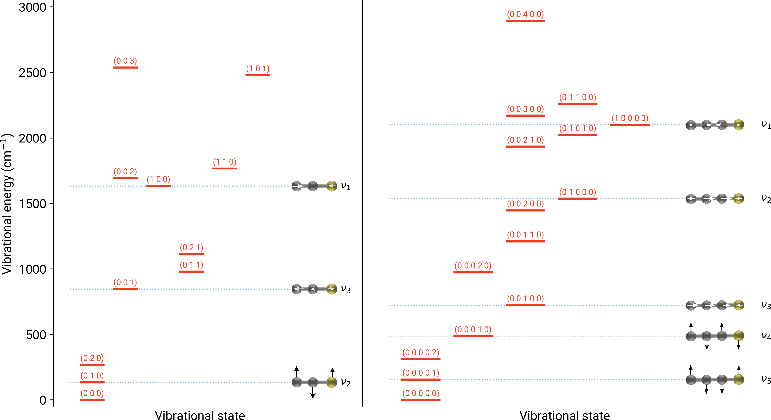
Fig.  1: Vibrational energy level diagram of C2S (left) and C3S (right). The mode deformation associated with each fundamental vibration is represented pictorially. Vibrational quantum numbers for each state are indicated using the convention ($v_{1}\ v_{2}\ v_{3}[\cdots]$) in which $v_{i}$ is the quanta of excitation in the $\nu_{i}$ modes. For brevity, the $l$ quantum number associated with the bending modes has been omitted. For C2S, levels for which pure rotational transitions have been observed in this work are shown with plain lines (in red), while some indicative levels which are not observed are represented with dashed lines (in gray). Owing to the high density of states for C3S, only observed and fundamental vibrational states are shown.

2.2 Microwave spectral taxonomy

In the centimeter-wave regime, FTMW techniques have been a workhorse of molecular spectroscopy for more than 30 years.²⁵ In either the CP or cavity variants of this method, a short pulse of microwave radiation, typically of order a few $\mu$s, creates a coherent macroscopic polarization, provided that one or molecules possesses a rotational transition in the FT-limited frequency bandwidth of the pulse. Because the timescale of the free-induction decay (FID) is typically at least an order of magnitude longer than the excitation step, the molecular signal can be detected with a sensitive microwave receiver in a ‘background-free’ regime. The Fourier-transform of the time-domain signal in combination with the frequency of the microwave radiation yields the precise frequencies of the rotational transitions.

Cavity FTMW spectroscopy is widely used because it provides high sensitivity, albeit with a very narrow instantaneous bandwidth, of order 0.5 MHz at each setting of the Fabry-Perot cavity. In contrast, CP-FTMW extends the instantaneous spectral coverage to many GHz — at a modest reduction (a factor of $\sim$40) in sensitivity and spectral resolution (a factor of $\sim$10) compared to the cavity variant — allowing the acquisition of enormous portions of a rotational spectrum simultaneously.¹⁰ Because CP-FTMW has a fairly flat instrumental response, relative abundances of multiple species can often be determined with far greater accuracy than with cavity measurements.

To exploit the unique strengths of CP-FTMW and cavity-FTMW, MST was recently developed. In this procedure, the chirped spectrum is first used as a survey tool to detect active, or ‘bright,’ resolution elements. The spectral features lying within the frequency range of the CP-FTMW spectrum (typically 2–8 or 8–18 GHz) are analyzed using a program such as SPECData, which is a newly developed in-house database query system that rapidly assigns transitions of known species, common contaminants, and instrumental artifacts, in a semi-automated fashion.²⁶ The remaining, unidentified features are then scrutinized using cavity spectroscopy for rapid characterization, because of its higher instantaneous sensitivity and spectral resolution. Part of this analysis is to categorize each spectral line based on a set of quantifiable properties: dipole moment; precursor dependence; magnet susceptibility; requirement of an excitation source (e.g., electrical discharge or laser ablation). Following classification, lines that share a common set of characteristics may be then subjected to exhaustive double resonance (DR) tests to determine those transitions that share a common upper or lower energy level, and thus arise from the same carrier. Previous studies of large aromatic compounds²⁷ found that only a handful of linkages may be needed to determine all three rotational constants of a molecule. Details of the two spectrometers used in the present investigation have been described in detail elsewhere¹¹, and will only be discussed briefly.

2.3 Centimeter-wave Measurements

In this study, CP-FTMW spectra were acquired in the 7.5–18 GHz band using several precursor combinations: a sulfur source (CS2) and one of two hydrocarbons (HCCH and HC4H), heavily diluted in argon, and then expanded in neon. The various gas mixtures, their concentrations, and total number of FIDs acquired in each experiment are summarized in Table 1. In all cases, the gas mixture was subject to a dc discharge just after the pulsed nozzle source, but prior to supersonic expansion into the large vacuum chamber. The pulsed nozzle was operated at a repetition rate of 5 kHz, the backing pressure behind the nozzle was 2.5 kTorr (333 kPa), and the discharge voltage was typically 1.5 kV. Finally, 10 FIDs were collected per gas pulse during the CP-FTMW measurements. In addition to recording spectra of the two CS2/hydrocarbon mixtures, spectra starting with only CS2 or HC4H were also acquired, to determine which species required the presence of both reactants.

After acquisition, features with a specified SNR (greater than five) were automatically flagged in each CP-FTMW spectrum, and subjected to further processing to identify those that coincided with transitions of well-known molecules or are instrumental in origin. Roughly 50% of the original features were removed in this step; the remaining features were then scrutinized further with a cavity FTMW spectrometer using essentially identical experimental conditions. A by-product of the cavity studies is improved frequency accuracy (2 kHz or better) compared with CP-FTMW spectroscopy, by roughly an order of magnitude (10 to 50). If a new series of nearly harmonically related lines was identified between 7.5 and 18 GHz, the measurements were routinely extended to 40 GHz in the cavity instrument with the same level of accuracy. Double resonance techniques were also used to extend measurements above the frequency range of the cavity instrument, providing that the higher-frequency line shared an energy level with a strong centimeter-wave line (see Tables A3 and A5).

Table 1: Precursor gases (diluted in Ar), mixing ratios, and number of averages collected in the CP-FTMW experiments.

Precursor Gases	Mixing Ratio${}^{a}$	dc voltage /kV	FIDs /million
2% CS2 : 0.75% HC4H	1:1:7	1.15	1.25
1% CS2 : 2% HCCH	3:6:5	1	1.60
2% CS2	1:9	1.15	1.25
0.75% HC4H	1:4	1.15	1.25

${}^{a}$ The buffer gas was Ne in each experiment and its ratio is the last value reported.

2.4 Millimeter-wave Measurements

Evidence for millimeter-wave lines of vibrationally excited C2S and C3S was found in archival spectra taken during previous searches for the HCCS ²⁸ and HC3S radicals²⁹. Spectra were acquired between 253 and 280 GHz using a 3 m long free space absorption spectrometer that has been described in detail previously ^{30, 31}, in which a low pressure (35 mTorr) dc discharge (200 mA) was struck through HCCH, CS2, and helium (He) in a molar ratio of 10:5:1, with the walls of the discharge cell cooled to 190 K using liquid nitrogen. In this frequency range, strong lines of both HCCS and HC3S were observed, as were lines of C2S and C3S. For C2S, two rotational transitions ($J^{\prime}=21-20$ and $20-19$) were covered, while five transitions ($J^{\prime}=48-44$) of C3S lie in the same frequency range due to its smaller rotational constant.

Tunable millimeter-wave radiation, generated by a phase-locked Gunn oscillator in combination with a frequency multiplier ($\times$2 or $\times$3), passed twice through the absorption cell to improve the SNR. Before entering the cell, radiation first passed through a grid polarizer and then, after passing through a lens, propagated along the length of the discharge cell where it was then reflected by a roof top mirror; reflection rotates the plane of polarization by 90${}^{\circ}$. After counter-propagating back through the cell, radiation was reflected by the grid polarizer and focused onto a sensitive, liquid He cooled indium antimonide (InSb) detector. To suppress 1/$f$ noise, frequency modulation combined with lock-in detection at $2f$ was used, resulting in line profiles that are well described by the second-derivative of a Lorentzian.

Because the Gunn oscillator is a resonant device with limited frequency agility, spectra were acquired in 200 MHz segments before the oscillator required manual re-tuning; the resulting segments were then concatenated together to produce a survey with continuous frequency coverage over many GHz. To distinguish between rotational lines of radicals and non-radicals, each frequency segment was recorded twice, once in the absence of a strong axial magnetic field, and then again in the presence of the magnetic field using otherwise identical conditions. By subtracting these two spectra, it is possible to identify only open-shell species such as C2S, as non-magnetic lines are typically subtracted out, with residuals at the level of a few percent. In contrast, lines of closed-shell C3S are expected to be present in both spectra. Because each rotational transition of C2S is magnetic and consists of a closely spaced triplet, this combination provided a distinct spectral signature for new lines of C2S, even though only two of its transitions fall in the range of the existing survey.

2.5 Quantum chemical calculations

Calculations of the molecular structures and vibration-rotation interactions were performed using the CFOUR suite of electronic structure programs. ³² The molecular geometries of C2S and C4S were optimized using coupled-cluster methods with single, double, and perturbative triple excitations [CCSD(T)], based on an unrestricted Hartree-Fock (UHF) reference wavefunction to treat the triplet multiplicity of these species. The calculations were performed with the frozen-core (fc) approximation using the correlation consistent basis sets of Dunning (i.e. cc-pVXZ). ³³ The geometry optimizations were converged to a root-mean-squared value for the molecular gradient to less than $10^{-7}$ hartrees/bohr. The resulting structures were verified to be minimum energy geometries by harmonic frequency analysis. Subsequently, the vibration-rotation coupling constants were calculated to first order ($\alpha_{i}$) using second-order vibrational perturbation theory (VPT2) as implemented in CFOUR, with the required cubic force-fields computed via finite-differences of analytic gradients.

The exothermocity of the reaction between linear C3 and S ($\mathrm{{}^{3}P}$) were calculated using the HEAT345(Q) scheme. The method is well-documented in previous publications,^{34, 35} and thus only briefly summarized here. The molecular geometries of linear C3 and C3S are first optimized at the ae-CCSD(T)/cc-pVQZ level of theory. Based on the structure obtained at this level, the HEAT345(Q) energy ($E_{\mathrm{HEAT}}$) is given by the sum of additive terms:

$$E_{\mathrm{HEAT}}=E^{\infty}_{\mathrm{HF}}+E^{\infty}_{\mathrm{CCSD(T)}}+E_{\Delta\mathrm{T-(T)}}+E_{\mathrm{(Q)}}+E_{\mathrm{ZPE}}+E_{\mathrm{DBOC}}+E_{\mathrm{Rel.}}$$ (1)

where $E^{\infty}_{\mathrm{HF}}$ and $E^{\infty}_{\mathrm{CCSD(T)}}$ are the extrapolated Hartree-Fock and CCSD(T) correlation contributions based on calculations with aug-cc-pCVXZ (where X=T,Q,5) basis, $E_{\Delta\mathrm{T-(T)}}$ is the extrapolated difference between the fc-CCSDT and fc-CCSD(T) energies with cc-pVXZ (where X=T,Q) basis, $E_{\Delta\mathrm{HLC}}$, $E_{(Q)}$ is the correlation contribution from perturbative quadruple excitations from an fc-CCSDT(Q)/cc-pVDZ calculation, $E_{\mathrm{ZPE}}$ is the harmonic zero-point energy, $E_{\mathrm{DBOC}}$ is the diagonal Born-Oppenheimer correction, and $E_{\mathrm{Rel.}}$ denotes the scalar relativistic corrections to the energy based sum of the mass-velocity, one and two-electron Darwin terms. Details on the extrapolation schemes used can be found in Reference 34. The CCSDT(Q) calculation was performed using the MRCC program interfaced with CFOUR. ³⁶

3 Results

Although there is considerable variance in the chemical richness of the four discharge mixtures (Table 2), all produce molecules of astronomical interest. While CS2 alone only yields the shortest carbon-sulfur chains (C2S to C4S) in detectable abundances, evidence was found for more than a dozen acetylenic free radicals, carbenes, and methyl polyynes in the HC4H discharge, nearly all of which have been detected in space. Addition of a hydrocarbon to a CS2 discharge results in a plethora of carbon and sulfur compounds, of which 36% have already been observed in space. As illustrated in Figure 2 and Tables 2–A2, one of the most striking features in the CS2/hydrocarbon discharges is the remarkably high SNR of small reactive species such as C3S, and the large number of newly identified lines close in frequency (within a few per cent) to these strong features. Indeed, the SNR is high enough for C3S that we were able to observe CCC^33S in natural abundance in both the CS2 + HC4H and CS2 + HCCH spectra, and assign its rotational spectrum for the first time (see Tables A10 & LABEL:ccc33s_freqs). Due to the high sensitivity of the measurements, evidence was routinely found for common contaminants such as SO2 and OCS in our chirped-pulse spectra. In particular, the CS2 + HCCH mixture experiment was performed immediately after an experiment using SO2 as a precursor, yielding strong lines of this species, its vibrational satellites, and isotopologues in the broadband spectrum. It is also worth noting a weak C3S line was detected in the CP-FTMW spectrum nominally containing only HC4H and carrier gas, a testimony to the ease with which C3S can be produced even when trace quantities of CS2 are apparently present.

Table 2: Pure hydrocarbon and sulfur-containing species identified in each reaction mixture whose frequencies were known prior to present work. Numbers in the Table represent the signal-to-noise ratio of the strongest line assigned for each species.

Species${}^{a}$	CS2 + HC4H	CS2 + HCCH	CS2	HC4H
C2S	161	75	19	3
CC${}^{34}$S	19	3	3
${}^{13}$CCS	2
C${}^{13}$CS	2
C3S	2040	598	18	18
$v_{1}=1\>^{d}$	16
$v_{4}=1^{1}\>{}^{d}$	138	67	3	2
$v_{5}=1^{1}\>{}^{d}$	3	17	2	2
$v_{3}=1$	130	76	3	2
CCC${}^{34}$S	109	23	2	2
${}^{13}$CCCS	19	3
C${}^{13}$CCS	18	5
C4S	302	19	5	5
C5S	125	103		4
C5 ^34S	7
C6S	12	3
C7S	20	12
C8S	3
HC3S	50	152		3
HC4S	215	110	2	3
HC5S	23	13		5
HC6S	17	17
HC7S	2	2
HC8S	5	2
H2C2S	2	5
H2C3S	21	35
H2C4S	17	23
H2C5S	6	12
H2C6S		3
HCSC2H	14	7
HCSC4H	9	11
$c$-C3H	13	23		54
C4H	20			171
C5H	26	9		230
C6H	3			49
C7H	4			77
C8H	3			60
C9H				32
C10H				7
C11H				4
$c$-C3H2	8	372		16
$v_{6}=1$	3	5		7
$v_{3}=1$		5
$v_{2}=1$		3
C${}^{13}$CHCH ${}^{b}$		3
C4H2	6			16
$l$-C5H2	3			35
$c$-C5H2	16	3		70
C5H2 ${}^{c}$				25
C6H2				3
C7H2				6
CH3C2H	17			9
CH3C4H	2	3		21
SH ${}^{e}$	2	48
$v=1$ ${}^{d}$		10

${}^{a}$ Main isotopologue in its ground vibrational state, unless otherwise noted.

${}^{b}$ Refers to the isotopic variant in which ${}^{13}$C has been substituted at one of the two equivalent carbon atoms.

${}^{c}$ Refers to the bent-chain isomer, i.e. isomer 3 in Ref. 37.

${}^{d}$ Centimeter-wave lines observed for the first time, using rotational constants determined from previous works ^{38, 39, 40}. See Tables A8 and LABEL:sh_cm_freq for a complete listing of observed transitions.

${}^{e}$ One additional hyperfine line reported compared to Ref. 41 (see Table LABEL:sh_cm_freq).

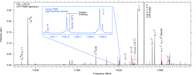
Fig.  2: A portion of the CP-FTMW spectrum obtained between 7.5 and 18 GHz, through an electrical discharge of dilute CS2 + HC4H in Ne/Ar, showing features near the $J=2-1$ transition of C3S. All C3S lines that have been assigned from the present analysis are labeled in black, with newly identified transitions highlighted in red. The intensity of the ground state C3S line has been truncated in this plot, to more easily illustrate less intense features, many of which are observed with high SNR; its peak value (4.1) is roughly 15 times that of the next strong feature in the frequency range. Lines that remain unidentified are marked with asterisks. The inset shows a high-resolution cavity FTMW spectrum of several closely-spaced transitions; owing to the Doppler effect, each line in this spectrum consists of a closely-spaced doublet.

Nearly all of the species observed in the CS2 + HC2H spectrum are also found in the CS2 + HC4H discharge, with the latter mixture generally resulting in much stronger lines for most carbon-rich molecules (Table 2). Because this mixture yields the richest array of compounds, it is the main focus of the spectral analysis presented here. In this spectrum, 59 unique variants (including isotopic and vibrational states) from 42 chemical species were assigned; among these are five vibrational satellite transitions of C3S and SH, which were observed in the centimeter domain for the first time using previously reported rotational constants (see Tables 2, A8, and LABEL:sh_cm_freq). Once transitions of these species were assigned in the CP spectra, exhaustive binary DR tests were performed on the remaining transitions to identify other features that might arise from a common carrier or carriers. Many DR linkages were found, but most connect only two lines separated by $\sim$5.8 GHz, implying a rotational constant close to that of C3S ($\sim$2.9 GHz), since this molecule has two transitions within the range of the CP-FTMW spectrum, one at 11.5 GHz ($J=2-1$) and another at 17 GHz ($J=3-2$), both of which lie close in frequency to the new DR linkages. Taken together, these findings strongly suggest the presence of many new vibrationally excited states of C3S. Surprisingly, some of the unidentified lines are comparably in intensity to lines from the $v_{5}=1^{1}$ (CCS bending), $v_{4}=1^{1}$ (CCC bending) and $v_{3}=1$ states of C3S, which were previously observed by Tang and Saito,³⁸ and Crabtree et al. ¹¹, respectively (see Fig 2).

Working under the operative assumption that these unidentified lines arise from still other vibrationally excited states of C3S, and that additional transitions should obey a simple linear-molecule progression, follow-up cavity measurements were undertaken to detect higher-frequency ($>$18 GHz) transitions. Because the predicted frequencies of the higher-$J$ lines are simply related to one another by ratios of integers, little search was required. On the basis of theoretical vibration-rotation constants calculated previously ⁴² and those in §2.5, nearly 20 series have now been assigned to vibrationally excited normal C3S or one it is more abundant isotopic species. Table 3 summarizes the newly-assigned transitions, while the measured centimeter-wave frequencies are given in Table A8.

Table 3: New states of C2S, C3S and C4S assigned in this work. Numbers in brackets indicate the signal-to-noise ratio of the strongest assigned transition of the state in the CS2 + HC4H reaction mixture chirped-pulse spectrum. Remaining states were observed only in the cavity instrument.

C2S		C3S						C4S
main		main		^13CCCS	C^13CCS	C${}_{3}^{\,34}$S	C${}_{3}^{\,33}$S	main	C${}_{4}^{\,34}$S
$v_{1}\leavevmode\nobreak\ =\leavevmode\nobreak\ 1$	$[19]$	$v_{2}\leavevmode\nobreak\ =\leavevmode\nobreak\ 1$		$v_{3}=1$	$v_{3}=1\;[3]$	$v_{3}=1\;[8]$	GS $[9]$	$v_{6}=1^{1}\;[8]$	GS $[7]$
$v_{2}\leavevmode\nobreak\ =\leavevmode\nobreak\ 1^{1}$		$v_{3}\leavevmode\nobreak\ =\leavevmode\nobreak\ 2$	$[24]$			$v_{4}=1\;[5]$		$v_{7}=1^{1}\;[5]$
$v_{2}\leavevmode\nobreak\ =\leavevmode\nobreak\ 2^{0}$		$v_{3}\leavevmode\nobreak\ =\leavevmode\nobreak\ 3$	$[7]$
$v_{3}\leavevmode\nobreak\ =\leavevmode\nobreak\ 1$	$[38]$	$v_{3}\leavevmode\nobreak\ =\leavevmode\nobreak\ 4$
$v_{3}\leavevmode\nobreak\ =\leavevmode\nobreak\ 2$		$v_{4}\leavevmode\nobreak\ =\leavevmode\nobreak\ 2^{0,2}$	$[28]$
$v_{3}\leavevmode\nobreak\ =\leavevmode\nobreak\ 3$		$(v_{1},v_{3})\leavevmode\nobreak\ =\leavevmode\nobreak\ (1,2)$	$[2]$
$(v_{1},v_{2})\leavevmode\nobreak\ =\leavevmode\nobreak\ (1,1^{1})$		$(v_{2},v_{3})\leavevmode\nobreak\ =\leavevmode\nobreak\ (1,1)$	$[10]$
$(v_{1},v_{3})\leavevmode\nobreak\ =\leavevmode\nobreak\ (1,1)$	$[6]$	$(v_{3},v_{4})\leavevmode\nobreak\ =\leavevmode\nobreak\ (1,1^{1})$	$[10]$
$(v_{2},v_{3})\leavevmode\nobreak\ =\leavevmode\nobreak\ (1^{1},1)$		$(v_{2},v_{4})\leavevmode\nobreak\ =\leavevmode\nobreak\ (1,1^{1})$	$[2]$
$(v_{2},v_{3})\leavevmode\nobreak\ =\leavevmode\nobreak\ (2^{0},1)$

Note: Transitions of C3S in $v_{1}=1$, $v_{4}=1$, $v_{5}=1,2$, and $(v_{1},v_{3})=(1,1)$ have also been observed for the first time in the centimeter domain using previously reported spectroscopic constants for these states^{38, 39}, see Table A8.

The presence of vibrationally excited lines of C3S in our spectra suggests that C2S and even C4S may be excited similarly. Only the $J_{N}=2_{1}-1_{0}$ transition of C2S near 11 GHz, however, lies in the frequency range of the CP-FTMW spectrum, with the next strong transition lying closer to 22 GHz; consequently, no new lines of C2S can be identified by DR using only the CP-FTMW coverage. Nevertheless, in CP-FTMW spectra where C3S lines are strong, vibrationally excited lines typically fall within a few % (i.e. a few 100 MHz near 11 GHz) of the ground state (see Fig. 2). To establish if some of the unidentified lines near 11 GHz arise from vibrationally excited C2S, surveys covering roughly $\pm 2$% in frequency around the $J_{N}=1_{2}-2_{1}$ transition of the ground state near 22 GHz were subsequently performed using cavity FTMW spectroscopy. Several unidentified lines were observed in this frequency region, and soon afterwards linked to low-frequency lines in the CP-FTMW spectrum by DR. Still higher-frequency transitions were then measured with the cavity spectrometer up to 40 GHz, and an additional line was often detected by DR spectroscopy between 40 and 60 GHz. On the basis of the close agreement between the measured lines and predictions from the vibration-rotation constants in §2.5, these lines have been assigned to the $\nu_{1}$ and $\nu_{2}$ stretching modes, two quanta of the $\nu_{3}$ bending mode, or some combination of the three. Table A3 summarizes the centimeter-wave measurements of the new vibrational states.

Although no DR linkages implicate new vibrationally excited states of C4S, careful inspection of the four rotational transitions that lie in our CP-FTMW spectra revealed a weak cluster of features displaced to slightly higher frequency compared to the ground state line for each transition. Subsequent assays, chemical tests, and DR measurements established that these lines behave as the ground state, and on the basis of the vibration-rotation constants given in Table 4, were assigned to the two lowest-frequency bending modes ($v_{6}=1$ and $v_{7}=1$); these transition frequencies are summarized in Table LABEL:c4s_cm_freqs. Under optimized experimental conditions, lines of $v_{6}=1$ are roughly 50 times weaker than the same lines of the ground state, while those of $v_{7}=1$ are closer to a 100 times weaker, implying T${}_{\rm vib}\sim 130$ K and $\sim 40$ K respectively. Despite the comparably high SNR of lines of C5S (Table 2), and some prior experimental work in the infrared,⁴³, no vibrationally excited lines were found for this species.

On the basis of the newly measured lines of vibrationally excited C2S and C3S at low frequency, predictions were then made between 253 and 280 GHz, a frequency region that coincides with a survey previously performed in a low pressure, long-path dc glow spectrometer (§2.4). Because the expected uncertainty in line positions obtained by extrapolation is only a few MHz at these frequencies, assignments of higher-$J$ transitions of vibrationally excited C2S ($J^{\prime}=20,21$) and C3S ($J^{\prime}=44-48$) were fairly straightforward (see Tables A5 and 1). Fits that combine both sets of measurements were then performed for each new state using the CALPGM (SPFIT/SPCAT) suite of programs.⁴⁴ The best-fit constants are given in Tables A6 and A10 for C2S and C3S, respectively; those for C4S are summarized in Table LABEL:c4s_constants. The data set for many vibrational states is limited to centimeter-wave measurements. In these cases, the centrifugal distortion constant $D$ was fixed to the value of the normal isotopic species.

In addition to vibrational satellite lines of C2S and C3S, transitions from vibrationally excited CS, C${}^{34}$S, ${}^{13}$CS, and C${}^{33}$S were also identified in the course of our re-analysis of the millimeter-wave survey. These measurements are summarized in Table LABEL:cs_vibstates.

4 Discussion

4.1 MST as a stepping stone for millimeter-wave assignment and astrophysical implications

The present work demonstrates a simple but highly useful aspect of MST – the ability to rapidly and confidently identify new vibrational satellite transitions of abundant, well-studied molecules in a reaction mixture containing familiar and transient species. As demonstrated here, an electrical discharge of two small-molecule precursors, CS2 and either HCCH or HC4H, produced a mixture of considerable complexity in which in excess of 70 unique chemical species, their more abundant isotopic variants and/or in their vibrationally excited states are present in detectable abundances; in total, 31 vibrational states or new isotopic were assigned for the first time. Because this reaction screening technique can be implemented relatively easily, it may be an appealing alternative to traditional methods for detecting new species of plausible astronomical interest, their isotopic species, and in vibrationally excited states. Although many transitions have been assigned, a large fraction ($\sim$40%) remain unidentified, implying the discovery space for entirely new compounds is still sizable.

The use of CP-FTMW spectroscopy as a tool for molecular discovery was illustrated several years ago in the astronomical identification of ethaninimine (CH3CHNH)³ and E-cyanomethanimine (HNCHCN).⁴⁵ In that study, a nearly identical discharge source was employed, and acetonitrile (CH3CN) and ammonia (NH3) were used as precursors. By directly comparing cm-wave CP-FTMW spectra to a frequency-coincident molecular line survey of the Sagittarius B2(N) star-forming region, several frequency coincidences were found, strongly suggesting a common carrier; subsequent laboratory work ultimately established the presence of both species in the interstellar medium (ISM) for the first time. Both CH3CHNH and HNCHCN, however, were studied at least to some extent in previous microwave investigations. ^{46, 47, 48} In this sense, MST extends previous efforts by its ability to systematically and rapidly identify lines that arise from a unique species, regardless of whether the identity of the carrier is known from prior work. In combination with theoretical calculations and other tests and assays, it is then often possible to deduce the elemental composition and structure of the carrier, as recent work on the isomers of H2C5O and other long-chain cumulenones demonstrates.⁴⁹

By performing laboratory measurements at centimeter wavelengths with a jet source, where the detection sensitivity and the spectral resolution are both very high, and spectral confusion is not an issue, measurements can be extended with little uncertainty to millimeter-wavelengths, where powerful millimeter-wave interferometers such as ALMA operate. Because spectral confusion is also much more common in laboratory spectra at these wavelengths, there is great practical utility in using microwave data as a ‘stepping stone’ to higher frequencies. The identification and assignment of a significant number of new transitions of C2S and C3S in legacy spectra from our laboratory are but one such example. Because the fits span both high and low-frequency data, transitions at intermediate frequencies can be trivially predicted with high accuracy.

Finally, the fairly exhaustive analysis of the microwave spectra by MST enables a comprehensive characterization of the chemical and physical processes that are operative in an electrical discharge starting with either CS2 alone, or in combination with a hydrocarbon, either HCCH or HC4H. Several examples highlighting this point are given in the sections that follow, including the formation pathways of C2S and C3S, their vibrational excitation, and the abundances of long-chain molecules in comparison to the ISM.

4.2 Formation of C2S and C3S

Following the detection of the simplest C${}_{n}$S thiocumulenes, C2S and C3S, in the ISM,^{22, 24} in the late 1980s, the formation pathways of these molecules and longer members has been a topic of considerable debate. While ion-neutral reactions involving S${}^{+}$ were originally believed to be sufficient to reproduce the observed abundances,⁵⁰ detailed modeling based on these reactions revealed a sizable discrepancy (of several orders of magnitude) between predicted and observed abundances in IRC+10216.^{51, 52} Subsequent theoretical investigations suggested that neutral-neutral and radical-neutral reactions likely play a significant role,^{53, 54} a supposition which has recently been supported by observations of unequal ${}^{13}$C ratios in C2S and C3S towards the cold, dark molecular cloud TMC-1.⁵⁵ Indeed, from the observed [C${}^{13}$CS]/[${}^{13}$CCS] abundance ratio of $\sim$4 in the cold molecular clouds TMC-1 and L1521E, Sakai et al.⁵⁵ concluded that reactions involving S/S${}^{+}$ are not the main pathway to C2S, and this species is instead likely formed from two reactants, each of which contributes a C atom. An analogous argument has been put forth for C3S ⁵⁶.

In the laboratory, it is well established from prior experiments that, as in the interstellar medium, S and CS are the major fragmentation products in an CS2 electrical discharge⁵⁷, and that the fractional ionization is very low, of order $10^{-5}$ or less, when a heavy inert atom such Ne and Ar is used as the buffer gas ⁵⁸. As a result, the steady-state abundance of S${}^{+}$ should be several orders of magnitude lower than atomic S, and the ion-molecule reactions probably contribute little to the operative chemistry.

Reactions between neutral and radical species are instead expected to dominate, where hydrocarbon fragments are likely formed via several competing reactions:

$$\ce{HCCH} \rightarrow 2\ \ce{CH}$$ (2)

$$\rightarrow \ce{C2H}+\ce{H}$$ (3)

$$\ce{HC4H} \rightarrow 2\ \ce{C2H}$$ (4)

$$\rightarrow \ce{C4H}+\ce{H}$$ (5)

$$\rightarrow \ce{C3H}+\ce{CH}$$ (6)

In our laboratory experiments, formation pathways for C2S include:

$$\ce{CH}+\ce{CS} \rightarrow \ce{C2S}+\ce{H}$$ (7)

$$\ce{C2H}+\ce{S} \rightarrow \ce{C2S}+\ce{H}$$ (8)

In fact, Eq. 7 is thought to be the most probable route to produce C2S in TMC-1.⁵⁵ Electrical discharge sources are notorious for their lack of specificity and rapid isotopic scrambling, and so we carried out C2S isotopic experiments with acetylene and ${}^{13}$CS2 in place of CS2, the results of which point to the importance of Eq. 8. Under our experimental conditions, relatively little ${}^{13}$C enhancement is observed for either ${}^{13}$CCS or C${}^{13}$CS, despite strong lines of normal CCS, an indication that the acetylenic unit remains largely intact during molecule formation, and that ${}^{13}$C from ${}^{13}$CS2 serves largely as a spectator. This finding is consistent with earlier laboratory studies by Ikeda et al. ⁵⁹ who first reported the rotational spectrum of ${}^{13}$CCS and C${}^{13}$CS. In that study, they concluded the C$\equiv$C bond in acetylene did not cleave efficiently, as the use of an enriched sample of H${}^{13}$C${}^{13}$CH did not result in stronger lines of either of the two ${}^{13}$C species. In fact, lines of the double-substituted species ${}^{13}$C${}^{13}$CS were readily observed instead.

The formation of C3S through the radical-radical recombination reaction

$$\ce{C2H}+\ce{CS}\rightarrow\ce{C3S}+\ce$$ (9)

would appear to be a particularly promising route to form C3S in our discharge experiments, since both radicals are known to be produced in high abundance from their respective precursors, and because radical-radical reactions are normally exothermic and barrierless. If a major pathway, it follows that the C-S bond should remain intact during molecule formation. Analogous experiments to those performed on C2S with ${}^{13}$CS2, however, suggest a different pathway to C3S than Eq. 4.2. Under a wide range of conditions, including low concentrations of both precursors and very low discharge voltages, ${}^{13}$C insertion appeared to occur facilely but with little selectively, with C${}^{13}$CCS or ${}^{13}$CCCS only at most a factor of two less abundant than CC${}^{13}$CS. Equally surprising was the presence of strong lines of normal C3S under the same conditions. Taken together, these findings suggest that: (1) C3 or a closely-related species such as C3H radical serves as a key reaction partner, but one that must be formed via a cyclic intermediate or transition state so as to produce a nearly statistically distribution of ${}^{13}$C in the carbon chain; and (2) a subsequent reaction with free sulfur then yields C3S. Previous experimental and theoretical studies conclude that the reaction:

$$\ce{C3}+\ce{H2}\rightarrow\ce{c-C3H2}$$ (10)

is the most energetically stable product channel starting from HCCH and either C(${}^{1}$D) or C(${}^{3}$P). This pathway is barrierless for C(${}^{1}$D) insertion, and while the same reaction with C(${}^{3}$P) is spin-forbidden, it is still thought to proceed efficiently via intersystem crossing ⁶⁰. If relevant to our discharge chemistry, this reaction may also help explain why ${}^{13}$C isotopic scrambling in longer hydrocarbon chains such as C5H, C6H, and C7H is so prevalent ⁶¹.

4.3 Vibrational Excitation

Molecules produced in high abundance in our discharge source frequently possess some degree of vibrational excitation, and C2S and C3S are no exception. As demonstrated in earlier studies ^{62, 63}, rotational satellite transitions from vibrationally excited states are commonly observed for small abundant molecules despite the very low rotational temperature in the jet expansion (typically $\sim$1-3 K). The vibrational distribution is highly non-thermal due to the competition between excitation, which includes collisions with electrons having an average kinetic energy of 1–3 eV and the excess internal energy that the molecule may possess as a result of formation, and relaxation which is dominated by collisional cooling. As a consequence of these two competing factors, vibrational modes that have frequencies much below room temperature can be efficiently cooled on the timescale of the expansion, while one or more modes usually lying slightly above room temperature are "frozen out"; lines from high-frequency stretches are uniformly weak, ostensibly because the density of states increases quickly with vibrational energy, and there is a commensurate increase in the rate of internal vibrational relaxation (IVR). Given the complexity of IVR processes in polyatomic molecules, it is almost impossible to predict details of this behavior in advance, especially when the formation pathway and internal energy distribution of the molecule are rarely known. Nevertheless, the degree of vibrational excitation in our discharge experiments tends to fall off quickly with increasing size of the molecule, and is only infrequently observed for carbon chains with more than about six heavy (carbon-like) atoms. For C5S, for example, no lines that could be attributed to vibrationally excited states were identified in our CP-FTMW spectra, despite detection of lines of C${}_{5}^{34}$S in natural abundance.

Because C3S has a ${}^{1}\Sigma^{+}$ ground state with a harmonically-related transitions, analysis of its rotational satellite transitions is fairly straightforward, and consequently many vibrational states from either the normal or its rare isotopic species were assigned for the first time (Table 3). As indicated in Fig. 2, transitions from $\nu_{3}$, the lowest-energy stretching mode, and the $\nu_{4}$ bend are particularly intense, regardless of whether acetylene or diacetylene is used as the hydrocarbon source. Excitation of $\nu_{3}$ is especially prominent in that states with as much as four quanta ($E\approx$2892 cm${}^{-1}$) have been assigned. Table 4 provides a comparison of the experimentally-derived vibration-rotation constants $\alpha_{i}$ to those predicted for C3S and C2S, in which $\alpha_{i}$ were obtained by differences of the rotational constants with respect to the ground state using the expression:

$$\Delta B=B_{0}-B_{v_{i}}\approx v_{i}\cdot\alpha_{i}$$ (11)

where $i$ refers to the mode $\nu_{i}$. For the $\nu_{3}$ mode, in which transitions from multiple quanta were observed, $\alpha_{3}$ was derived from linear regression as a function of the vibrational quantum number, $v_{3}$ (Fig. 3) this analysis yields a precise, best-fit value within 10% of that predicted from Seeger et al.⁴².

How excess energy is partitioned among the five vibrational modes of C3S may provide clues as to its formation mechanism. It is perhaps not surprising that significant energy would be concentrated in the $\nu_{3}$ mode (Fig. 4) because it involves motion of the C–S unit, and the reaction of S atom with C3 (or a hydrocarbon fragment with the same number of C atoms) has been implicated as an important pathway to form C3S: based on our calculations with HEAT345(Q) thermochemistry, the association of C3 + S -> C3S is highly exothermic (-594.8 kJ mol${}^{-1}$). Regarding how the reaction may occur, we can attempt to speculate on a mechanism based on the observed partitioning of this excess energy. As seen in Figure 4, vibrational temperatures of order 700 K are found for $\nu_{3}$ and $\nu_{4}$. This effective temperature is remarkably similar to those previously derived in our laboratory for chains such as HC3N. ⁶³ Assuming the reaction proceeds barrierlessly, as is typical for radical-radical recombination reactions, the excess energy should be partitioned statistically. While the vibrational temperatures of $\nu_{3}$ and $\nu_{4}$ are comparable and therefore suggestive of a statistical distribution of states, the remaining vibrational modes ($\nu_{1}$, $\nu_{2}$, and $\nu_{3}$) are also observed, but are much less intense. However, as mentioned earlier in this section, vibrations with frequencies that deviate from room temperature significantly are generally cooled efficiently, or scrambled through IVR. Given the large body of experimental measurements that are now available for C3S, it may be feasible to construct an accurate global potential energy surface, and trajectory simulations may prove enlightening.

Table 4: Theoretical and experimental vibration-rotation ($\alpha_{i}$) interaction constants of C2S, C3S, and C4S (in MHz).

Iso.	Vib.	$\alpha_{i}$
Species	Mode	Theory ${}^{a}$	Experiment
C2S	$v_{1}$	$46.6$	$47.1$
	$v_{2}$	$19.0$	$20.0$
	$v_{3}$	$-27.8$	$-29.7$
C3S	$v_{1}$	$15.2\;^{b}$	$14.8\>^{c}$
	$v_{2}$	$11.1\>^{b}$	$11.2$
	$v_{3}$	$4.2\>^{b}$	$3.79$
	$v_{4}$	$-5.2\>^{b}$	$-5.6\>^{d}$
	$v_{5}$	$-11.2\>^{b}$	$-12.4\>^{d}$
C4S	$v_{1}$	$6.81$
	$v_{2}$	$4.86$
	$v_{3}$	$3.52$
	$v_{4}$	$1.34$
	$v_{5}$	$-1.88$
	$v_{6}$	$-2.62$	$-2.61$
	$v_{7}$	$-3.28$	$-3.07$

${}^{a}$ Unless otherwise noted, the theoretical constants were calculated at the fc-CCSD(T)/cc-pVDZ level of theory.

${}^{b}$ Ref. 42

${}^{c}$ Ref. 39.

${}^{d}$ Ref. 38.

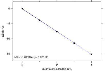
Fig.  3: Differences between the rotational constants of C3S ($\Delta B=B_{v}-B_{0}$) in the ground and vibrationally excited levels of the $\nu_{3}$ mode versus vibrational quantum number, $v_{3}$. The experimental value for $\alpha_{3}$ was determined from a least-squares optimization (blue trace, $r$= 0.99997; see text).

C2S possesses a ${}^{3}\Sigma^{-}$ ground state with a very large spin-spin constant ($\lambda$), which makes a detailed analysis of its vibrational excitation more challenging because the transitions are not strictly related to one another by ratios of integers at low $J$. Nevertheless, rotational lines from 10 vibrational states have been assigned either in our CP-FTMW spectra or in subsequent cavity searches at higher frequency, guided by theoretical calculations of the vibration-rotation coupling constants (§2.5). These include either the fundamental or overtone of each mode or some combination of the three. This degree of excitation appears fairly common for small molecules, e.g. triatomics, that are either produced or subjected to an electrical discharge. Strong satellites transitions are frequently observed in most or all of the vibrational modes, presumably because coupling between modes is relatively inefficient due to a low density of states, and because rotational spectra of many small molecules can frequently be observed with very high SNRs. Although evidence was also found for all five vibrational modes of C3S, several are very weak in our spectra. In contrast, only two modes of C4S and no modes of C5S were found under the same experimental conditions, strongly suggesting that IVR plays a prominent role in rapidly and efficiently dissipating internal energy. The experimental $\alpha$’s derived for each state of C2S compare quite favorably to those calculated (Table 4), indicating that the current theoretical treatment is adequate.

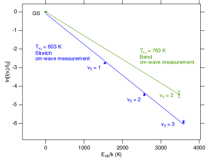
Fig.  4: Vibrational temperature diagram of $\nu_{4}$ and $\nu_{3}$ of C3S in the cm-wave CP-FTMW spectra. Error bars (1$\sigma$) arise from uncertainties in the intensities that were derived from Gaussian fits to the line profiles.

4.4 Production of Longer Sulfur-Terminated Carbon-Chains

The longest carbon chains detected in the ISM are C8H/C8H^-, HC9N, C3S, and HC5O, for hydrogen, nitrogen, sulfur, and oxygen-bearing species, respectively.^{64, 65, 66, 67, 68, 69, 70} In TMC-1, for example, lines of single ${}^{13}$C-C3S have been reported, but no evidence has been found for C5S, despite the availability of precise laboratory rest frequencies ⁷¹ for more than 20 years, and construction of new single-dish telescopes, such as the 100 m GBT telescope, which have even greater collecting area. A tentative detection has been reported at higher frequencies in IRC+10216.⁷² In contrast, radio lines of neutral and negatively-charged acetylenic chains as long as C8H/C8H^- have been found in TMC-1. Under our experimental conditions, spectra of chains as long as C7S and C8H are simultaneously observed in CP-FTMW spectra, suggesting there is no obvious kinetic or thermodynamic obstacle to formation of sulfur-terminated chains beyond C3S. Rather, the stability of C3S combined with the well-known depletion of sulfur in dense, cold molecular clouds (at the level of 99.9% relative to the cosmic value⁷³) point to elemental abundance as a mitigating factor in the production of longer sulfur-terminated chains in this source.

4.5 Further Analysis

Despite attempts to comprehensively analyze the spectra of hydrocarbon-sulfur discharges, about 40% of the lines in our CP-FTMW spectra with a SNR in excess of 3 remain unassigned; the strongest of these are observed with a SNR close to 100. Undoubtedly some fraction of these lines arise from still higher quanta or combination modes of normal and isotopic C2S, C3S and C4S or other abundant discharge molecules, such as HC3S, HC(S)C${}_{2}$H, etc. while others may arise from relatively light molecules such as $c$-C3H2, which only possess a single transition in the 8–18 GHz frequency range of the CP-FTMW spectrometer. Because these features will have no DR matches in the measurement range, further analysis and assignment is challenging. Some of the strongest unidentified lines in the HC4H discharge, for example, were recently assigned to one or more quanta in the $v_{6}$ mode of $c$-C3H2 in an unrelated study ⁷⁴. To more easily identify light molecules and more routinely detect multiple DR linkages of the same molecule, a three-band system for CP-FTMW operating between 2 and 26.5 GHz will soon be implemented.

5 Conclusions

An extensive MST analysis of several hydrocarbon/CS2 discharges has revealed the presence of many vibrationally excited states of C2S, C3S, and C4S. Subsequent analysis using new or existing theoretical vibration-rotation constants has enabled a total 27 new vibrational states of the three chains to be assigned; in combination with previously identified species, 90 unique products were assigned in the CS2 + HC4H discharge. Predictions from the centimeter-wave data allowed previously unidentified lines of these species in archival millimeter-wave data to be identified and assigned with confidence. In this way, complete and accurate spectral catalogs of species over the entire range of interest to radio astronomers can be compiled for subsequent use in analyzing complex interstellar mixtures. This approach is particularly appealing for vibrationally excited species, which serve as excellent probes of physical conditions in the ISM, and offer access to different spatial scales than their ground vibrational state counterparts, particularly in regions where the lowest-energy species is optically thick. Finally, isotopic spectroscopy using ${}^{13}$CS${}_{2}$ indicated that the dominant formation pathway for C2S in our laboratory discharge likely proceeds through C2H + S, while C3S appears to be formed from a cyclic intermediate, since ${}^{13}$C is found to be nearly randomly distributed along the chain.

Table A1: Ab initio vibrational frequencies and first order vibration-rotation coupling constants ($\alpha$) for ground state C2S ($\tilde{X}\leavevmode\nobreak\ ^{3}\Sigma^{-}$) and C4S ($\tilde{X}\leavevmode\nobreak\ ^{3}\Sigma^{-}$) computed at the fc-CCSD(T)/cc-pVDZ level of theory using VPT2. Frequencies are given in cm${}^{-1}$ while $\alpha$ is provided in MHz.

Species	Mode	Harmonic frequency	Anharmonic frequency	$\alpha$
C2S	$\nu_{1}$	$1782.41$	$1632.77$	$46.62$
	$\nu_{3}$	$847.36$	$845.79$	$18.95$
	$\nu_{2}$	$257.25$	$134.03$	$-27.79$
C4S	$\nu_{1}$	$2085.17$	$2043.99$	$6.82$
	$\nu_{2}$	$1783.96$	$1743.71$	$4.87$
	$\nu_{3}$	$1207.79$	$1208.14$	$3.52$
	$\nu_{4}$	$602.86$	$575.73$	$1.34$
	$\nu_{5}$	$519.47$	$290.92$	$-1.50$
	$\nu_{6}$	$326.01$	$266.97$	$-2.50$
	$\nu_{7}$	$129.15$	$112.42$	$-3.21$

Table A2: Oxygen-, nitrogen-, sulfur-, and argon-containing species identified in each reaction mixture whose frequencies were known prior to present work. Numbers in the Table represent the signal-to-noise ratio of the strongest line assigned for each species.

Species${}^{a}$	CS2 + HC4H	CS2 + HCCH	CS2	HC4H
C3O		5		21
C5O				3
HC3O	13	2		9
HC4O	7			15
HC5O				3
HC6O				3
HC7O				3
H2CO	4			8
H2C5O	7			8
CH3CHO		99
CH3OCHO		71
HCOC2H	6	5		7
C2H5OH		2
OH		2
SO2	2	163
$v_{1}=1$		17
$v_{2}=1$		77
$v_{2}=2$		29
$v_{2}=3$		3
$(v_{1},v_{2})=(1,1)$		12
^34SO2		11
HC3N		4		3
HC5N	9			15
HC7N				3
CH3CN		3
CH3NO		3
H2O–H2O	3	2	5
H2O–HC2H		3
H2O–HC4H	11
OCS	5	6	2
SNO		3

${}^{a}$ Main isotopologue in its ground vibrational state, unless otherwise noted.

Table A3: Measured centimeter-wave transitions of the ground and vibrationally excited normal and isotopic C2S (in MHz).

Iso.	Vib.	Transition, $J^{\prime}_{N^{\prime}}-J^{\prime\prime}_{N^{\prime\prime}}$
Species	State	$2_{1}-1_{0}$	$1_{2}-2_{1}$	$2_{3}-1_{2}$	$3_{4}-2_{3}$	$2_{2}-1_{1}$	$3_{2}-0_{1}$	$3_{3}-2_{2}$
C${}_{2}^{\,34}$S	GS ${}^{a}$		$21930.4756$	$33111.8370$
C2S	$(v_{1},v_{3})=(1,1)$	$11027.0403$	$22154.5032$	$33457.0705$	$44971.725$
C2S	$v_{3}=3$	$11053.8201$	$22205.5507$	$33528.4000$	$45059.175$
C2S	$v_{1}=1$	$11036.2863$	$22177.3620$	$33500.5144$	$45043.037$
C2S	$v_{3}=2$	$11078.3628$	$22256.5671$	$33609.0152$
C2S	$v_{3}=1$	$11102.8764$	$22307.6307$	$33689.9173$	$45287.000$
C2S	$(v_{1},v_{2})=(1,1^{1})$	$-$	$22125.9220$	$33452.0276$	$45019.275$
		$-$	$22179.3904$	$33530.1076$	$45120.400$
C2S	GS ${}^{a}$	$11119.4452$	$22344.0305$	$33751.3699$	$45379.020$	$25911.015$	$29477.700$	$38866.417$
C2S	$(v_{3},v_{2})=(1,1^{1})$	$-$	$22270.2587$	$33658.5184$	$45280.525$
		$-$	$22323.5767$	$33736.5616$	$45381.850$
C2S	$v_{2}=1^{1}$	$-$	$22304.5697$	$33718.0178$	$45371.475$
		$-$	$22357.3069$	$33795.1252$	$45471.425$
C2S	$(v_{2},v_{3})=(2^{0},1)$	$11158.0445$	$22425.5719$	$33882.7887$	$45567.600$
C2S	$v_{2}=2^{0}$	$11174.1680$	$22461.5174$	$33944.4177$	$45661.000$

Note: Estimated measurement uncertainties are 2 kHz below 40 GHz. Above this frequency, transitions have been measured using double resonance techniques resulting in a 25 kHz uncertainty. For states with $l=1$, the $2_{1}-1_{0}$ transition is not allowed, as indicated by a dash symbol in the corresponding lines.

${}^{a}$ Several centimeter-wave lines were previously reported with a higher uncertainty in Refs. 22 and 75.

Table A4: Measured centimeter–wave transitions of ${}^{13}$C isotopologues of C2S (in MHz).

$N^{\prime}_{J^{\prime}}\leavevmode\nobreak\ -\leavevmode\nobreak\ N^{\prime\prime}_{J^{\prime\prime}}$	$F^{\prime}\leavevmode\nobreak\ -\leavevmode\nobreak\ F^{\prime\prime}$	${}^{13}$CCS	C${}^{13}$CS
$2_{1}\leavevmode\nobreak\ -\leavevmode\nobreak\ 1_{0}$	$0.5\leavevmode\nobreak\ -\leavevmode\nobreak\ 0.5$	$10699.9518$	$11078.4014$
	$1.5\leavevmode\nobreak\ -\leavevmode\nobreak\ 0.5$	$10706.9119$	$11075.2940$
$1_{2}\leavevmode\nobreak\ -\leavevmode\nobreak\ 2_{1}$	$1.5\leavevmode\nobreak\ -\leavevmode\nobreak\ 1.5$	$21487.4534$	$22259.7156$
	$1.5\leavevmode\nobreak\ -\leavevmode\nobreak\ 0.5$	$21494.4117$	$22256.6071$
	$2.5\leavevmode\nobreak\ -\leavevmode\nobreak\ 1.5$	$21498.6616$	$22254.7319$
$2_{3}\leavevmode\nobreak\ -\leavevmode\nobreak\ 1_{2}$	$2.5\leavevmode\nobreak\ -\leavevmode\nobreak\ 1.5$	$32440.1924$	$33615.1718$
	$3.5\leavevmode\nobreak\ -\leavevmode\nobreak\ 2.5$	$32443.9526$	$33613.5400$

Note: Estimated measurement uncertainties are 2 kHz. Several centimeter-wave lines were previously reported with a higher uncertainty in Ref. 59.

Table A5: Measured millimeter-wave transitions in the ground, $v_{1}=1$ and $v_{3}=1$ vibrationally excited states of C2S (in MHz).

$J^{\prime}_{N^{\prime}}\leavevmode\nobreak\ -\leavevmode\nobreak\ J^{\prime\prime}_{N^{\prime\prime}}$	GS${}^{a}$	$v_{1}=1$	$v_{3}=1$
$0_{1}\leavevmode\nobreak\ -\leavevmode\nobreak\ 1_{2}$	162749.178
$1_{1}\leavevmode\nobreak\ -\leavevmode\nobreak\ 2_{1}$	183257.261	181634.082	184483.054
$2_{2}\leavevmode\nobreak\ -\leavevmode\nobreak\ 1_{2}$	186824.217
$0_{1}\leavevmode\nobreak\ -\leavevmode\nobreak\ 1_{0}$	196212.630
$3_{2}\leavevmode\nobreak\ -\leavevmode\nobreak\ 2_{1}$	214570.887
$20_{19}\leavevmode\nobreak\ -\leavevmode\nobreak\ 19_{18}$	258274.283	256395.149	257460.718
$20_{20}\leavevmode\nobreak\ -\leavevmode\nobreak\ 19_{19}$	259055.427		258254.193
$20_{21}\leavevmode\nobreak\ -\leavevmode\nobreak\ 19_{20}$	259700.932	257811.769	258910.073
$21_{20}\leavevmode\nobreak\ -\leavevmode\nobreak\ 20_{19}$	271292.242	269318.144	270439.575
$21_{21}\leavevmode\nobreak\ -\leavevmode\nobreak\ 20_{20}$	272002.244		271160.971
$21_{22}\leavevmode\nobreak\ -\leavevmode\nobreak\ 20_{21}$	272592.955	270610.151	271761.284

Note: Estimated measurement uncertainties are 25 kHz. Transitions below 250 GHz have been measured using double resonance technique in the cavity FT instrument.

${}^{a}$ Some of these transitions were previously reported by Refs. 22 and 75 with a 20 kHz uncertainty.

Table A6: Spectroscopic constants of the ground and vibrationally excited normal and isotopic C2S (in MHz, sorted by increasing $B$ value or by isotopic variant).

Iso.	Vib.	$B$	$10^{3}D$	$\gamma$	$10^{3}\gamma_{D}$	$\lambda$	$10^{3}\lambda_{D}$	$q/2$	$p/2$	N${}^{a}$	weighted
Species	State										ave.${}^{b}$
${}^{13}$CCS	GS ${}^{c}$	6188.0867(4)	1.5720(5)	-14.06(1)	0.037	97204.0(2)	24.5(3)			56	0.83
C${}_{2}^{\;34}$S	GS	6335.8839(3)	1.6543(5)	-14.386(7)	0.037	97195.1(1)	26.8(2)			30	0.99
C2S	$(v_{1},v_{3})=(1,1)$	6411.057(4)	1.7271	-14.711	0.037	97323.7(3)	27.0			4	0.22
C2S	$v_{3}=3$	6417.230(4)	1.7271	-14.711	0.037	98259.4(4)	27.0			4	0.62
C2S	$v_{1}=1$	6430.6293(3)	1.7271	-12.353(3)	0.037	96341.31(1)	27.0			9	0.57
C2S	$v_{3}=2$	6437.336(4)	1.7271	-14.711	0.037	98039.0(4)	27.0			3	0.19
C${}^{13}$CS	GS ${}^{c}$	6446.9655(5)	1.7119(7)	-14.63(1)	0.037	97226.7(2)	28.1(4)			45	0.79
C2S	$v_{3}=1$	6457.7175(2)	1.7271	-14.542(3)	0.037	97800.18(1)	27.0			11	1.11
C2S	$(v_{1},v_{2})=(1,1^{1})$	6460.987(3)	1.7271	-14.711	0.037	94920.1(2)	27.0	-4.597(5)	-26.47(3)	6	4.51
C2S	GS	6477.7496(2)	1.7271(3)	-14.711(2)	0.037(5)	97195.651(6)	27.0(2)			52	0.78
C2S	$(v_{2},v_{3})=(1^{1},1)$	6487.104(3)	1.7271	-14.711	0.037	96699.5(3)	27.0	-4.716(5)	-25.79(3)	6	3.67
C2S	$v_{2}=1^{1}$	6507.496(3)	1.7271	-14.711	0.037	96077.5(3)	27.0	-4.609(5)	-25.72(3)	6	3.58
C2S	$(v_{2},v_{3})=(2^{0},1)$	6513.254(4)	1.7271	-14.711	0.037	96614.2(3)	27.0			4	0.54
C2S	$v_{2}=2^{0}$	6534.040(4)	1.7271	-14.712	0.037	95972.5(3)	27.0			4	0.35
C2S	GS	6477.7496(2)	1.7271(3)	-14.711(2)	0.037(5)	97195.651(6)	27.0(2)			52	0.78
	$v_{1}=1$	6430.6293(3)	1.7271	-12.353(3)	0.037	96341.31(1)	27.0			9	0.57
	$v_{2}=1^{1}$	6507.496(3)	1.7271	-14.711	0.037	96077.5(3)	27.0	-4.609(5)	-25.72(3)	6	3.58
	$v_{2}=2^{0}$	6534.040(4)	1.7271	-14.712	0.037	95972.5(3)	27.0			4	0.35
	$v_{3}=1$	6457.7175(2)	1.7271	-14.542(3)	0.037	97800.18(1)	27.0			11	1.11
	$v_{3}=2$	6437.336(4)	1.7271	-14.711	0.037	98039.0(4)	27.0			3	0.19
	$v_{3}=3$	6417.230(4)	1.7271	-14.711	0.037	98259.4(4)	27.0			4	0.62
	$(v_{1},v_{2})=(1,1^{1})$	6460.987(3)	1.7271	-14.711	0.037	94920.1(2)	27.0	-4.597(5)	-26.47(3)	6	4.51
	$(v_{1},v_{3})=(1,1)$	6411.057(4)	1.7271	-14.711	0.037	97323.7(3)	27.0			4	0.22
	$(v_{2},v_{3})=(1^{1},1)$	6487.104(3)	1.7271	-14.711	0.037	96699.5(3)	27.0	-4.716(5)	-25.79(3)	6	3.67
	$(v_{2},v_{3})=(2^{0},1)$	6513.254(4)	1.7271	-14.711	0.037	96614.2(3)	27.0			4	0.54
C${}_{2}^{\;34}$S	GS	6335.8839(3)	1.6543(5)	-14.386(7)	0.037	97195.1(1)	26.8(2)			30	0.99
${}^{13}$CCS	GS ${}^{c}$	6188.0867(4)	1.5720(5)	-14.06(1)	0.037	97204.0(2)	24.5(3)			56	0.83
C${}^{13}$CS	GS ${}^{c}$	6446.9655(5)	1.7119(7)	-14.63(1)	0.037	97226.7(2)	28.1(4)			45	0.79

Note: Uncertainties (1$\sigma$) are in units of the last significant digit. Best-fit constants derived from pure rotational frequencies reported in the literature^{22, 75, 59} and line frequencies in Tables A3, A4, and A5, using a standard linear molecule Hamiltonian in a ${}^{3}\Sigma$ electronic state, with or without $l$-type doubling. Values with no associated uncertainties were constrained to the value derived for the normal isotopic species. We note that the RMS values involving the $\nu_{2}$ state are significantly larger than those for other vibrational states. This difference arises in part due to the small dataset combined with the need to include several lambda-doubling terms. A smaller RMS should be achieved by varying additional terms, but, for simplicity, we have chosen to report a fit in which only the leading constants were varied, and are well determined.

${}^{a}$ Refers to the number of lines in the fit.

${}^{b}$ Dimensionless.

${}^{c}$ The ${}^{13}$C hyperfine terms $b$ and $c$ are omitted here and are reported in Table A7

Table A7: Hyperfine spectroscopic constants of ${}^{13}$C isotopic variants of C2S (in MHz),

Parameter	${}^{13}$CCS	C${}^{13}$CS
$b$	$18.6(6)$	$-19.2(6)$
$c$	$-50.(2)$	$-16.(2)$

Table A8: Measured centimeter-wave transitions of the ground and vibrationally excited normal and isotopic C3S (in MHz).

Iso.	Vib.	Transition, $J^{\prime}-J^{\prime\prime}$
Species	State	$2-1$	$3-2$	$4-3$	$5-4$	$6-5$
${}^{13}$CCCS	$v_{3}=1$	11117.8715	16676.7930	22235.7098	27794.5918	33353.4555
${}^{13}$CCCS	GS	11132.2395${}^{a}$	16698.3481${}^{a}$	22264.4418${}^{a}$	27830.5140${}^{a}$	33396.5590
C${}_{3}^{\,34}$S	$v_{3}=1$	11266.5956	16899.8806	22533.1503	28166.3989	33799.6182
C${}_{3}^{\,34}$S	GS	11281.468${}^{b}$	16922.1924${}^{a}$	22562.8997${}^{a}$	28203.5870${}^{a}$	33844.2426
C${}_{3}^{\,34}$S	$v_{4}=1^{1}$	11300.6585	16950.9732	22601.2722	28251.5511	33901.8087
		11306.4008	16959.5927	22612.7667	28265.9189	33919.0458
C${}^{13}$CCS	$v_{3}=1$	11430.3317	17145.4856	22860.6204	28575.7375	34290.8264
C${}^{13}$CCS	GS	11445.4767${}^{a}$	17168.2027${}^{a}$	22890.9123${}^{a}$	28613.6016${}^{a}$	34336.2592
C${}_{3}$S	$(v_{1},v_{3})=(1,2)$	11470.6766	17206.0013	22941.3100	28676.5972	34411.8556
C${}_{3}$S	$(v_{1},v_{3})=(1,1)\,^{d,e}$	11486.9578	17230.4235	22973.8700	28717.2944
		11487.0135	17230.5062	22973.9831	28717.4367
C${}_{3}$S	$v_{3}=4$	11500.9602	17251.4245	23001.8723	28752.2983
C${}_{3}$S	$(v_{2},v_{3})=(1,1)$	11501.4629	17252.1815	23002.8831	28753.5630	34504.2175
C${}_{3}$S	$v_{1}=1\,^{e}$	11502.2624	17253.3805	23004.4807	28755.5607	34506.6142
C${}_{3}$S	$v_{3}=3$	11515.8557	17273.7704	23031.6688	28789.5478	34547.3957
C${}_{3}$S	$v_{2}=1$	11516.7518	17275.1133	23033.4615	28791.7862
C${}_{3}$S	$v_{3}=2$	11530.9586	17296.4249	23061.8746	28827.3029	34592.7057
C${}_{3}$S	$(v_{2},v_{4})=(1,1^{1})$	11535.7961	17303.6763	23071.5442	28839.3851	34607.2016
		11541.8122	17312.7127	23083.5936	28854.4462	34625.2725
C${}_{3}$S	$v_{3}=1$	11546.1972${}^{c}$	17319.283${}^{c}$	23092.3522${}^{c}$	28865.4002${}^{c}$	34638.4213${}^{c}$
C${}_{3}$S	GS	11561.5099${}^{a}$	17342.2564${}^{a}$	23122.9836${}^{a}$	28903.6913${}^{a}$	34684.3676
C${}_{3}$S	$(v_{3},v_{4})=(1,1^{1})$	11568.3746	17352.5444	23136.7006	28920.8350	34704.9434
		11574.9783	17362.4574	23149.9186	28937.3568	34724.7708
C${}_{3}$S	$v_{4}=1^{1}\,{}^{f}$	11581.0824	17371.6094	23162.1189	28952.6085	34743.0697
		11587.1082	17380.6511	23174.1755	28967.6795	34761.1548
C${}_{3}$S	$v_{5}=1^{1}\,{}^{f}$	11602.8885	17404.3150	23205.7261	29007.1130	34808.4727
		11618.7422	17428.1009	23237.4398	29046.7555	34856.0407
C${}_{3}$S	$v_{4}=2^{0}$	11603.1367	17404.6924	23206.2315	29007.7498	34809.2416
C${}_{3}$S	$v_{4}=2^{2}$	–	17409.7432	23212.9647	29016.1635	34819.3362
C${}_{3}$S	$v_{5}=2^{0\,^{f}}$	11660.5482	17490.7982	23321.0138	29151.1892

Note: This work, unless otherwise noted. Estimated measurement uncertainties are 2 kHz. Previously identified isotopic species and vibrationally excited states are included for completeness.

${}^{a}$ Ref. 76.

${}^{b}$ Ref. 77.

${}^{c}$ Ref. 11.

${}^{d}$ A closely-spaced doublet was observed. The centroid was used in the least-squares fit.

${}^{e}$ First observation of the centimeter-wave transitions; assignments based on the infrared measurements in Ref. 39.

${}^{f}$ First observation of the centimeter-wave transitions; assignments based on the millimeter observations in Ref. 38.

Table A9:  Measured millimeter-wave transitions of C3S (in MHz).

$J^{\prime}\leavevmode\nobreak\ -\leavevmode\nobreak\ J^{\prime\prime}$	GS${}^{a}$	$v_{3}=1$	$v_{3}=2$	$v_{4}=1^{a}$	$v_{4}=2^{0}$	$v_{4}=2^{2,\leavevmode\nobreak\ b}$	$v_{5}=1^{a}$	$v_{5}=2^{0\,a}$	$(v_{3},v_{4})=(1,1^{1})$
$44\leavevmode\nobreak\ -\leavevmode\nobreak\ 43$	254277.025	253940.217	253605.042	254706.569	255194.240	255261.620	255181.712	256384.431
				254839.022		255264.687	255526.635		254573.768
$45\leavevmode\nobreak\ -\leavevmode\nobreak\ 44$	260052.472	259708.080	259365.169	260491.715	260990.594	261059.157	260977.450	262204.508	260206.900
				260627.185		$\cdots$	261330.010
$46\leavevmode\nobreak\ -\leavevmode\nobreak\ 45$	265827.668	265475.613		266276.624	266786.708	266856.464	266772.916	268024.150
				266415.084		266860.017	267133.140		266137.984
$47\leavevmode\nobreak\ -\leavevmode\nobreak\ 46$	271602.622	271242.975		272061.270	272582.580	272653.499	272568.145	273843.340
				272202.742		272657.295	272935.981		271919.853
$48\leavevmode\nobreak\ -\leavevmode\nobreak\ 47$	277377.316	277009.990	276644.223	277845.724	278378.196	278450.302
				277990.158		278454.324

$J^{\prime}\leavevmode\nobreak\ -\leavevmode\nobreak\ J^{\prime\prime}$	C${}_{3}\>^{34}$S${}^{a}$	${}^{13}$CCCS	C${}^{13}$CCS
$44\leavevmode\nobreak\ -\leavevmode\nobreak\ 43$	253755.288
$45\leavevmode\nobreak\ -\leavevmode\nobreak\ 44$	259390.744		257443.430
$46\leavevmode\nobreak\ -\leavevmode\nobreak\ 45$	265025.964	255960.830	263160.721
$47\leavevmode\nobreak\ -\leavevmode\nobreak\ 46$		261521.591	268877.730
$48\leavevmode\nobreak\ -\leavevmode\nobreak\ 47$		267082.092	274594.608
$49\leavevmode\nobreak\ -\leavevmode\nobreak\ 48$		272642.376
$50\leavevmode\nobreak\ -\leavevmode\nobreak\ 49$		278202.381

Note: Estimated measurement uncertainties are 25 kHz.

${}^{a}$ Several of the Lines were previously reported in Refs. ^{24, 38}.

${}^{b}$ Centroid used in least-squares fit.

Table A10: Spectroscopic constants of the ground and vibrationally excited normal and isotopic C3S (in MHz, sorted by increasing $B$ values or by isotopic species).

Iso. Species	Vib. State	$B_{v}$	$10^{3}D_{v}$	$10^{9}H_{v}$	$q/2$	$10^{6}q_{J}/2$	Weighted ave.${}^{a}$	$N^{b}$
${}^{13}$CCCS	GS	2783.06176(6)	0.20782(3)	0.063			0.62	11
${}^{13}$CCCS	$v_{3}=1$	2779.4698(3)	0.211(5)	0.063			1.40	5
C${}_{3}^{\,34}$S	$v_{3}=1$	2816.6510(1)	0.22441	0.063			0.45	5
C${}_{3}^{\,34}$S	GS	2820.36928(6)	0.21389(2)	0.063			1.05	20
C${}_{3}^{\,34}$S	$v_{4}=1^{1}$	2825.8842(1)	0.212(2)	0.063	0.71829(5)		0.64	10
C${}_{3}^{\,33}$S	GS${}^{d}$	2854.3868(2)	0.222(4)	0.063			1.12	9
C${}^{13}$CCS	$v_{3}=1$	2857.5849(1)	0.22441	0.063			0.49	5
C${}^{13}$CCS	GS	2861.37104(6)	0.21959(3)	0.063			0.98	9
C${}_{3}$S	$(v_{1},v_{3})=(1,2)$	2867.6709(1)	0.22441	0.063			0.30	5
C${}_{3}$S	$(v_{1},v_{3})=(1,1)$	2871.7479(1)	0.22441	0.063			0.61	4
C${}_{3}$S	$v_{3}=4$	2875.2412(1)	0.22441	0.063			0.83	4
C${}_{3}$S	$v_{1}=1$	2875.5673(1)	0.22441	0.063			0.23	5
C${}_{3}$S	$(v_{2},v_{3})=(1,1)$	2875.3676(1)	0.22441	0.063			0.18	5
C${}_{3}$S	$v_{3}=3$	2878.9658(1)	0.22441	0.063			0.41	5
C${}_{3}$S	$v_{2}=1$	2879.1898(1)	0.22441	0.063			0.36	4
C${}_{3}$S	$v_{3}=2$	2882.7415(1)	0.22392(5)	0.063			0.46	8
C${}_{3}$S	$(v_{2},v_{4})=(1,1^{1})$	2884.7028(1)	0.22441	0.063	0.7530(1)		1.46	10
C${}_{3}$S	$v_{3}=1$	2886.5512(1)	0.22387(4)	0.063			1.06	11
C${}_{3}$S	GS	2890.38018(5)	0.22441(2)	0.063(4)			0.93	41
C${}_{3}$S	$v_{4}=1^{1}$	2896.02580(5)	0.22756(2)	0.079(3)	0.75353(3)	-0.238(5)	0.93	92
C${}_{3}$S	$(v_{3},v_{4})=(1,1^{1})$	2892.92123(7)	0.2317(6)	2.6(2)	0.82607(7)	0.41(4)	0.77	14
C${}_{3}$S	$v_{5}=1^{1}$	2902.70573(7)	0.24674(3)	0.138(5)	1.98217(5)	-5.735(9)	0.91	88
C${}_{3}$S	$v_{4}=2^{0}$	2900.7860(1)	0.22007(4)	0.063			0.10	10
C${}_{3}$S	$v_{4}=2^{2}$	2901.6282(1)	0.23533(4)	0.063			0.38	8
C${}_{3}$S	$v_{5}=2^{0\,c}$	2915.1410(1)	0.4398(1)	1.40(5)			0.71	43
C${}_{3}$S	GS	2890.38018(5)	0.22441(2)	0.063(4)			0.93	41
	$v_{1}=1$	2875.5673(1)	0.22441	0.063			0.23	5
	$v_{2}=1$	2879.1898(1)	0.22441	0.063			0.36	4
	$v_{3}=1$	2886.5512(1)	0.22387(4)	0.063			1.06	11
	$v_{3}=2$	2882.7415(1)	0.22392(5)	0.063			0.46	8
	$v_{3}=3$	2878.9658(1)	0.22441	0.063			0.41	5
	$v_{3}=4$	2875.2412(1)	0.22441	0.063			0.83	4
	$v_{4}=1^{1}$	2896.02580(5)	0.22756(2)	0.079(3)	0.75353(3)	-0.238(5)	0.93	92
	$v_{4}=2^{0}$	2900.7860(1)	0.22007(4)	0.063			0.10	10
	$v_{4}=2^{2}$	2901.6282(1)	0.23533(4)	0.063			0.38	8
	$v_{5}=1^{1}$	2902.70573(7)	0.24674(3)	0.138(5)	1.98217(5)	-5.735(9)	0.91	88
	$v_{5}=2^{0\,c}$	2915.1410(1)	0.4398(1)	1.40(5)			0.71	43
	$(v_{1},v_{3})=(1,1)$	2871.7479(1)	0.22441	0.063			0.61	4
	$(v_{1},v_{3})=(1,2)$	2867.6709(1)	0.22441	0.063			0.30	5
	$(v_{2},v_{3})=(1,1)$	2875.3676(1)	0.22441	0.063			0.18	5
	$(v_{2},v_{4})=(1,1^{1})$	2884.7028(1)	0.22441	0.063	0.7530(1)		1.46	10
	$(v_{3},v_{4})=(1,1^{1})$	2892.92123(7)	0.2317(6)	2.6(2)	0.82607(7)	0.41(4)	0.77	14
C${}_{3}^{\,34}$S	GS	2820.36928(6)	0.21389(2)	0.063			1.05	20
	$v_{3}=1$	2816.6510(1)	0.22441	0.063			0.45	5
	$v_{4}=1^{1}$	2825.8842(1)	0.212(2)	0.063	0.71829(5)		0.64	10
${}^{13}$CCCS	GS	2783.06176(6)	0.20782(3)	0.063			0.62	11
	$v_{3}=1$	2779.4698(3)	0.211(5)	0.063			1.40	5
C${}^{13}$CCS	GS	2861.37104(6)	0.21959(3)	0.063			0.98	9
	$v_{3}=1$	2857.5849(1)	0.22441	0.063			0.49	5
C${}_{3}^{\,33}$S	GS${}^{d}$	2854.3868(2)	0.222(4)	0.063			1.12	9

Note: Uncertainties (1$\sigma$) are in units of the last significant digit. Best-fit constants derived from line frequencies in Tables A8 & 1 and available pure rotational data from the literature^{77, 56, 24, 38, 11}, using a standard linear molecule ${}^{1}\Sigma$ Hamiltonian, either with or without $l$-type doubling. Values with no associated uncertainties were constrained to the value of the normal isotopic species.
${}^{a}$ Dimensionless.
${}^{b}$ Refers to the number of lines in the fit.
${}^{c}$ An additional CD-term, $L=0.207(6)\times 10^{-12}$ MHz, was required to fit the dataset to experimental accuracy.
${}^{d}$ Hyperfine constant: $\chi_{aa}$(S) = -15.889(9) MHz.

References

- Taatjes et al. 2008 C. A. Taatjes, N. Hansen, D. L. Osborn, K. Kohse-Höinghaus, T. A. Cool and P. R. Westmoreland, Phys. Chem. Chem. Phys., 2008, 10, 20–34.
- Semmelroch and Grosch 1995 P. Semmelroch and W. Grosch, LWT - Food Science and Technology, 1995, 28, 310–313.
- Loomis et al. 2013 R. A. Loomis, D. P. Zaleski, A. L. Steber, J. L. Neill, M. T. Muckle, B. J. Harris, J. M. Hollis, P. R. Jewell, V. Lattanzi, F. J. Lovas, O. J. Martinez, M. C. McCarthy, A. J. Remijan, B. H. Pate and J. F. Corby, The Astrophysical Journal Letters, 2013, 765, L9.
- Kowalsick et al. 2014 A. Kowalsick, N. Kfoury, A. Robbat, S. Ahmed, C. Orians, T. Griffin, S. B. Cash and J. R. Stepp, Journal of Chromatography A, 2014, 1370, 230 – 239.
- Teixeira and Rodrigues 2014 M. A. Teixeira and A. E. Rodrigues, Industrial & Engineering Chemistry Research, 2014, 53, 9875–9882.
- Daniel et al. 2011 R. Daniel, G. Tian, H. Xu, M. L. Wyszynski, X. Wu and Z. Huang, Fuel, 2011, 90, 449–458.
- Rosatella et al. 2011 A. A. Rosatella, S. P. Simeonov, R. F. M. Frade and C. A. M. Afonso, Green Chem., 2011, 13, 754–40.
- Wu et al. 2009 X. Wu, Z. Huang, T. Yuan, K. Zhang and L. Wei, Combustion and Flame, 2009, 156, 1365–1376.
- Togbé et al. 2014 C. Togbé, L.-S. Tran, D. Liu, D. Felsmann, P. Oßwald, P.-A. Glaude, B. Sirjean, R. Fournet, F. Battin-Leclerc and K. Kohse-Höinghaus, Combustion and Flame, 2014, 161, 780–797.
- Brown et al. 2008 G. G. Brown, B. C. Dian, K. O. Douglass, S. M. Geyer, S. T. Shipman and B. H. Pate, Rev Sci Instrum, 2008, 79, 053103–14.
- Crabtree et al. 2016 K. N. Crabtree, M.-A. Martin-Drumel, G. G. Brown, S. A. Gaster, T. M. Hall and M. C. McCarthy, J Chem Phys, 2016, 144, 124201–13.
- Garrod et al. 2008 R. T. Garrod, S. L. W. Weaver and E. Herbst, Astrophys J, 2008, 682, 283–302.
- Belloche et al. 2016 A. Belloche, H. S. P. Müller, R. T. Garrod and K. M. Menten, Astronomy & Astrophysics, 2016, 587, A91–66.
- Jørgensen et al. 2016 J. K. Jørgensen, M. van der Wiel, A. Coutens, J. Lykke, H. Muller, E. van Dishoeck, H. Calcutt, P. Bjerkeli, T. Bourke, M. Drozdovskaya, E. Fayolle, C. Favre, R. Garrod, S. Jacobsen, K. Öberg, M. Persson and S. Wampfler, Astronomy & Astrophysics, 2016, 595, A117.
- Cernicharo et al. 2013 J. Cernicharo, F. Daniel, A. Castro-Carrizo, M. Agúndez, N. Marcelino, C. Joblin, J. R. Goicoechea and M. Guélin, ApJ, 2013, 778, L25–6.
- Fortman et al. 2012 S. M. Fortman, J. P. McMillan, C. F. Neese, S. K. Randall, A. J. Remijan, T. L. Wilson and F. C. De Lucia, J Mol Spectrosc, 2012, 280, 11–20.
- Cernicharo et al. 2010 J. Cernicharo, L. B. F. M. Waters, L. Decin, P. Encrenaz, A. G. G. M. Tielens, M. Agúndez, E. De Beck, H. S. P. Müller, J. R. Goicoechea, M. J. Barlow, A. Benz, N. Crimier, F. Daniel, A. M. di Giorgio, M. Fich, T. Gaier, P. García-Lario, A. de Koter, T. Khouri, R. Liseau, R. Lombaert, N. Erickson, J. R. Pardo, J. C. Pearson, R. Shipman, C. Sánchez Contreras and D. Teyssier, A&A, 2010, 521, L8.
- Cernicharo et al. 2008 J. Cernicharo, M. Guélin, M. Agúndez, M. C. McCarthy and P. Thaddeus, The Astrophysical Journal, 2008, 688, L83.
- Müller et al. 2016 H. S. P. Müller, B. J. Drouin, J. C. Pearson, M. H. Ordu, N. Wehres and F. Lewen, Astronomy & Astrophysics, 2016, 586, A17–6.
- Carroll et al. 2010 P. B. Carroll, B. J. Drouin and S. L. Widicus Weaver, The Astrophysical Journal, 2010, 723, 845–849.
- Medvedev and de Lucia 2007 I. R. Medvedev and F. C. de Lucia, ApJ, 2007, 656, 621–628.
- Saito et al. 1987 S. Saito, K. Kawaguchi, S. Yamamoto, M. Ohishi, H. Suzuki and N. Kaifu, Astrophysical Journal, 1987, 317, L115–L118.
- Hirahara et al. 1993 Y. Hirahara, Y. Ohshima and Y. Endo, Astrophysical Journal, 1993, 408, L113–L115.
- Yamamoto et al. 1987 S. Yamamoto, S. Saito, K. Kawaguchi, N. Kaifu, H. Suzuki and M. Ohishi, Astrophysical Journal, 1987, 317, L119–L121.
- Balle and Flygare 1981 T. J. Balle and W. H. Flygare, Review of Scientific Instruments, 1981, 52, 33–45.
- Oliveira et al. 2017 J. Oliveira, M.-A. Martin-Drumel and M. C. McCarthy, SPECData: Automated Analysis Software for Broadband Spectra, 2017, For the current version, see https://github.com/jnicoleoliveira/SPECData.
- Martin-Drumel et al. 2016 M.-A. Martin-Drumel, M. C. McCarthy, D. Patterson, B. A. McGuire and K. N. Crabtree, J Chem Phys, 2016, 144, 124202.
- Vrtilek et al. 1992 J. M. Vrtilek, C. A. Gottlieb, E. W. Gottlieb, W. Wang and P. Thaddeus, Astrophysical Journal, 1992, 398, L73–L76.
- McCarthy et al. 1994 M. C. McCarthy, J. M. Vrtilek, E. W. Gottlieb, F.-M. Tao, C. A. Gottlieb and P. Thaddeus, The Astrophysical Journal Letters, 1994, 431, L127–L130.
- McCarthy et al. 1995 M. C. McCarthy, C. A. Gottlieb, A. L. Cooksy and P. Thaddeus, The Journal of Chemical Physics, 1995, 103, 7779–7787.
- Gottlieb et al. 2003 C. A. Gottlieb, P. C. Myers and P. Thaddeus, The Astrophysical Journal, 2003, 588, 655.
- Stanton et al. 2017 J. F. Stanton, J. Gauss, L. Cheng, M. E. Harding, D. A. Matthews, A. A. A. Szalay, P G, R. J. Bartlett, U. Benedikt, C. Berger, D. E. Bernholdt, Y. J. Bomble, O. Christiansen, F. Engel, R. Faber, M. Heckert, O. Heun, C. Huber, T. C. Jagau, D. Jonsson, J. Juselius, K. Klein, W. J. Lauderdale, F. Lipparini, T. Metzroth, L. A. Muck, D. P. O’Neill, D. R. Price, E. Prochnow, C. Puzzarini, K. Ruud, F. Schiffmann, W. Schwalbach, C. Simmons, S. Stopkowicz, A. Tajti, J. Vazquez, F. Wang and J. D. Watts, CFOUR, Coupled-Cluster techniques for Computational Chemistry, 2017, For the current version, see http://www.cfour.de.
- Dunning 1989 T. J. Dunning, The Journal of Chemical Physics, 1989, 90, 1007–1023.
- Harding et al. 2008 M. E. Harding, J. Vazquez, B. Ruscic, A. K. Wilson, J. Gauss and J. F. Stanton, Journal of Chemical Physics, 2008, 128, 114111.
- Bomble et al. 2006 Y. J. Bomble, J. Vazquez, M. Kallay, C. Michauk, P. G. Szalay, A. G. Csaszar, J. Gauss and J. F. Stanton, Journal of Chemical Physics, 2006, 125, 064108.
- Kállay et al. 2017 M. Kállay, Z. Rolik, J. Csontos, P. Nagy, G. Samu, D. Mester, J. Csóka, I. Ladjánszki, L. Szegedy, B. Ladóczki, K. Petrov, M. Farkas and B. Hégely, MRCC, a quantum chemical program suite, 2017, See www.mrcc.hu.
- Gottlieb et al. 1998 C. A. Gottlieb, M. C. McCarthy, V. D. Gordon, J. M. Chakan, A. J. Apponi and P. Thaddeus, The Astrophysical Journal Letters, 1998, 509, L141.
- Tang and Saito 1995 J. A. Tang and S. Saito, J Mol Spectrosc, 1995, 169, 92–107.
- Dudek et al. 2017 J. B. Dudek, T. Salomon, S. Fanghänel and S. Thorwirth, Int. J. Quantum Chem., 2017, 117, e25414–12.
- Martin-Drumel et al. 2012 M. A. Martin-Drumel, S. Eliet, O. Pirali, M. Guinet, F. Hindle, G. Mouret and A. Cuisset, Chemical Physics Letters, 2012, 550, 8–14.
- Meerts and Dymanus 1975 W. L. Meerts and A. Dymanus, Canadian Journal of Physics, 1975, 53, 2123–2141.
- Seeger et al. 1994 S. Seeger, P. Botschwina, J. Flügge, H. P. Reisenauer and G. Maier, Journal of Molecular Structure: THEOCHEM, 1994, 303, 213–225.
- Thorwirth et al. 2017 S. Thorwirth, T. Salomon, S. Fanghänel, J. R. Kozubal and J. B. Dudek, Chemical Physics Letters, 2017, 684, 262–266.
- Pickett 1991 H. M. Pickett, J Mol Spectrosc, 1991, 148, 371–377.
- Zaleski et al. 2013 D. P. Zaleski, N. A. Seifert, A. L. Steber, M. T. Muckle, R. A. Loomis, J. F. Corby, O. J. Martinez, K. N. Crabtree, P. R. Jewell, J. M. Hollis, F. J. Lovas, D. Vasquez, J. Nyiramahirwe, N. Sciortino, K. Johnson, M. C. McCarthy, A. J. Remijan and B. H. Pate, The Astrophysical Journal Letters, 2013, 765, L10.
- Lovas et al. 1980 F. J. Lovas, R. D. Suenram, D. R. Johnson, F. O. Clark and E. Tiemann, J Chem Phys, 1980, 72, 4964–10.
- Brown et al. 1980 R. D. Brown, P. D. Godfry and D. A. Winkler, Australian Journal of Chemistry, 1980, 33, 1.
- Takano et al. 1990 S. Takano, M. Sugie, K.-i. Sugawara, H. Takeo, C. Matsumura, A. Masuda and K. Kuchitsu, J Mol Spectrosc, 1990, 141, 13–22.
- McCarthy et al. 2017 M. C. McCarthy, L. Zou and M.-A. Martin-Drumel, The Journal of Chemical Physics, 2017, 146, 154301.
- Smith et al. 1988 D. Smith, N. G. Adams, K. Giles and E. Herbst, Astronomy & Astrophysics, 1988, 200, 191–194.
- Millar and Herbst 1990 T. J. Millar and E. Herbst, Astronomy & Astrophysics, 1990, 231, 466–472.
- Cernicharo et al. 1987 J. Cernicharo, C. Kahane, M. Guélin and H. Hein, Astronomy & Astrophysics, 1987, 181, L9–L12.
- Yamada et al. 2002 M. Yamada, Y. Osamura and R. I. Kaiser, Astronomy & Astrophysics, 2002, 395, 1031–1044.
- Petrie 1996 S. Petrie, Monthly Notices of the Royal Astronomical Society, 1996, 281, 666–672.
- Sakai et al. 2007 N. Sakai, M. Ikeda, M. Morita, T. Sakai, S. Takano, Y. Osamura and S. Yamamoto, ApJ, 2007, 663, 1174–1179.
- Sakai et al. 2013 N. Sakai, S. Takano, T. Sakai, S. Shiba, Y. Sumiyoshi, Y. Endo and S. Yamamoto, The Journal of Physical Chemistry A, 2013, 117, 9831–9839.
- Seaver et al. 1982 M. Seaver, J. W. Hudgens and J. D. Corpo, Chemical Physics, 1982, 70, 63 – 68.
- Lattanzi et al. 2010 V. Lattanzi, C. A. Gottlieb, P. Thaddeus, S. Thorwirth and M. C. McCarthy, The Astrophysical Journal, 2010, 720, 1717.
- Ikeda et al. 1997 M. Ikeda, Y. Sekimoto and S. Yamamoto, J Mol Spectrosc, 1997, 185, 21–25.
- Casavecchia et al. 2002 P. Casavecchia, N. Balucani, L. Cartechini, G. Capozza, A. Bergeat and G. G. Volpi, Faraday Discuss., 2002, 119, 27–49.
- McCarthy and Thaddeus 2005 M. C. McCarthy and P. Thaddeus, The Journal of Chemical Physics, 2005, 122, 174308.
- Sanz et al. 2003 M. E. Sanz, M. C. McCarthy and P. Thaddeus, J Chem Phys, 2003, 119, 11715–14.
- Sanz et al. 2005 M. E. Sanz, M. C. McCarthy and P. Thaddeus, J Chem Phys, 2005, 122, 194319–10.
- Cernicharo and Guélin 1996 J. Cernicharo and M. Guélin, Astronomy & Astrophysics, 1996, 309, L27.
- Remijan et al. 2007 A. J. Remijan, J. M. Hollis, F. J. Lovas, M. A. Cordiner, T. J. Millar, A. J. Markwick-Kemper and P. R. Jewell, The Astrophysical Journal, 2007, 664, L47.
- Brünken et al. 2007 S. Brünken, H. Gupta, C. A. Gottlieb, M. C. McCarthy and P. Thaddeus, ApJ, 2007, 664, L43–L46.
- Broten et al. 1978 N. W. Broten, T. Oka, L. W. Avery, J. M. MacLeod and H. W. Kroto, Astrophysical Journal, 1978, 223, L105–L107.
- Loomis et al. 2016 R. A. Loomis, C. N. Shingledecker, G. Langston, B. A. McGuire, N. M. Dollhopf, A. M. Burkhardt, J. Corby, S. T. Booth, P. B. Carroll, B. Turner and A. J. Remijan, Monthly Notices of the Royal Astronomical Society, 2016, 463, 4175–4183.
- Matthews et al. 1984 H. E. Matthews, W. M. Irvine, P. Friberg, R. D. Brown and P. D. Godfrey, Nature, 1984, 310, 125–126.
- McGuire et al. 2017 B. A. McGuire, A. M. Burkhardt, C. N. Shingledecker, S. V. Kalenskii, E. Herbst, A. J. Remijan and M. C. McCarthy, The Astrophysical Journal Letters, 2017, 843, L28.
- Kasai et al. 1993 Y. Kasai, K. Obi, Y. Ohshima, Y. Hirahara, Y. Endo, K. Kawaguchi and A. Murakami, Astrophysical Journal, 1993, 410, L45–L47.
- Agúndez et al. 2014 M. Agúndez, J. Cernicharo and M. Guélin, Astronomy & Astrophysics, 2014, 570, A45–9.
- Tieftrunk et al. 1994 A. Tieftrunk, G. Pineau des Forets, P. Schilke and C. M. Walmsley, Astronomy & Astrophysics, 1994, 289, 579–596.
- Gupta et al. 2017 H. Gupta, J. H. Baraban, B. Changala, S. Thorwirth, J. F. Stanton, M.-A. Martin-Drumel, O. Pirali, C. A. Gottlieb and M. C. McCarthy, International Symposium On Molecular Spectroscopy, 72nd Meeting, Abstract WF08.
- Yamamoto et al. 1990 S. Yamamoto, S. Saito, K. Kawaguchi, Y. Chikada, H. Suzuki, N. Kaifu, S. Ishikawa and M. Ohishi, The Astrophysical Journal, 1990, 361, 318–324.
- Sakai and Yamamoto 2013 N. Sakai and S. Yamamoto, Chemical Reviews, 2013, 113, 8981–9015.
- Ohshima and Endo 1992 Y. Ohshima and Y. Endo, J Mol Spectrosc, 1992, 153, 627–634.
- Gordon et al. 2001 V. D. Gordon, M. C. McCarthy, A. J. Apponi and P. Thaddeus, ApJS, 2001, 134, 311–317.
- Ahrens and Winnewisser 1999 V. Ahrens and G. Winnewisser, Zeitschrift für Naturforschung, 1999, 54a, 131–136.