Kinetic signature of cooperativity in the irreversible collapse of a polymer

Abstract

We investigate the kinetics of a polymer collapse due to the formation of irreversible crosslinks between its monomers. Using the contact probability $P(s)$ as a scale-dependent order parameter depending on the chemical distance $s$, our simulations show the emergence of a cooperative pearling instability. Namely, the polymer undergoes a sharp conformational transition to a set of absorbing states characterized by a length scale $\xi$ corresponding to the mean pearl size. This length and the transition time depend on the polymer equilibrium dynamics and the crosslinking rate. We confirm experimentally this transition using a DNA conformation capture experiment in yeast.

The collapse dynamic of a polymer chain has motivated multiple theoretical and experimental investigations (De Gennes, 1985; Grosberg et al., 1988; Chu et al., 1995; Buguin et al., 1996; Ostrovsky et al., 2001; Pitard and Bouchaud, 2001; Dokholyan et al., 2002; Halperin and Goldbart, 2000; Bunin and Kardar, 2015; Majumder et al., 2017). The seminal work of de Gennes, considering a collapse caused by solvent quality reduction with no effects of topological constraints, predicted a continuous conformational transition through successive crumpling stages commonly called the “expanding sausage model”  (De Gennes, 1985). Grosberg et al. proposed a two-stage model, where a fast collapse is followed by a slow unknotting of topological constraints through reptation (Grosberg et al., 1988). The meta-stable intermediate state, called “fractal-globule”, preserves the fractal features of a coil while being compact as a globule. The predicted existence of meta-stability was experimentally confirmed by Chu et al. (Chu et al., 1995). The stability of the fractal globule has been investigated in theoretical studies, which quantified the relaxation of this state towards an equilibrium globule (Schram et al., 2013; Chertovich and Kos, 2014). As another description of polymer collapse, Buguin et al. introduced the concept of pearling through the existence of a characteristic size, there explained by nucleation theory  (Buguin et al., 1996). Pearling has been subsequently studied in different works (Halperin and Goldbart, 2000; Pitard and Bouchaud, 2001; Ostrovsky et al., 2001; Dokholyan et al., 2002; Majumder et al., 2017). More recently Bunin and Kardar proposed an effective model of polymer collapse, consisting in a cascading succession of coalescence events of blobs actively compressed in a central potential (Bunin and Kardar, 2015).

All these studies investigate the collapse of a polymer under a deep quench: i.e. starting from an equilibrium conformation, interactions between the monomers are abruptly changed and the system relaxes to a new equilibrium state. Memory about the collapse process is lost in this final state. In contrast, we here study the collapse dynamics of a chain when it is caused by the cumulative effect of irreversible crosslinks between monomers, in the spirit of the pioneering study by Lifshitz, Grosberg, and Khokhlov (1976). In this case, crosslinks cannot be undone and the final state depends on the collapse dynamics. This process has important applications in materials science (e.g. vulcanization) and in molecular biology (e.g. cell fixation).

In order to describe the system, we consider here a scale-dependent order parameter: the contact probability curve $P_{t}(s)$, defined as the mean number of crosslinks present at time $t$ between two monomers at a chemical distance $s$. This order parameter has two important advantages: it reflects the appearance of local structures such as pearls, and it is a direct observable in the chromosome conformation capture experiments described at the end of this letter.

We run a rejection kinetic Monte Carlo simulation (Cacciuto and Luijten, 2006; Scolari and Lagomarsino, 2015) reproducing the Rouse phenomenology on 2048 beads connected initially by a linear chain of links of maximum length $b$. Each time two non-linked beads come in close vicinity (i.e. their distance fall less then $r_{int}=b/64$), a new link is made with a probability $p$ reflecting the crosslinking rate (details in Supplementary Materials (SM) §I.A). These links are then treated exactly as the links between consecutive monomers in the chain.

In the absence of crosslinking, the correlations of bead positions along time and along the chain satisfy the Rouse scaling relations with coefficients $C_{t}$ and $C_{s}$ (Doi and Edwards, 1988):

$$\begin{split}\left\langle\left|\vec{R}(0,t_{0})-\vec{R}(0,t+t_{0})\right|^{2}\right\rangle&\sim C_{t}\cdot t^{1/2},\\ \left\langle\left|\vec{R}(s_{0},0)-\vec{R}(s+s_{0},0)\right|^{2}\right\rangle&\sim C_{s}\cdot s.\end{split}$$ (1)

After thermal equilibration of the chain, crosslinking is introduced as a succession of irreversible and configuration-dependent changes in the chain topology. As a proxy for steric constraints, we limit the crosslink events to a maximum number per bead, $N_{max}$, known as the monomer functionality, and stop the simulation once this number is reached for all the beads. $N_{max}$ is equal to $4$ in the figures if not otherwise specified.

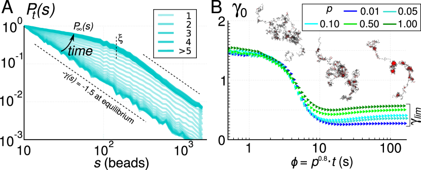
Figure 1: Kinetics of the pearling transition (simulation). (A) Time evolution of the contact probability curve $P_{t}(s)$ at fixed crosslink probability $p=0.1$, displayed as a superposition of semitransparent plots obtained at increasing simulation time $t$ (black arrow); the resulting color density is given in the inset. A crossover at a length $\xi$ arises at large enough times. Error bars are smaller than the thickness of the line. (B) Evolution of $\gamma_{0}$, the short-distance slope of the log-log plot of the $P_{t}(s)$, as a function of the rescaled time variable $\phi$, for different values of $p$. Inset: snapshots of the time evolution of the polymer conformation ($p=0.1$).

Given this dynamics, the contact probability $P_{t}(s;p,C_{s},C_{t})$ is a function of $s$, the crosslink probability $p$, the Rouse coefficients and the elapsed time $t$ from the crosslinking onset. At constant $p$, the time evolution of this curve displays a transition from the equilibrium contact probability, scaling as $\propto s^{-\gamma}$ with $\gamma={3/2}$, (De Gennes, 1980), to an asymptotic shape $P_{\infty}(s)$ displaying a crossover between two different scaling behaviors at short and long chemical distances  (Fig. 1A). This shape and the crossover length $\xi$ reflect the population average features of the absorbing states reached by the polymer at crosslink saturation. The exponent $\gamma_{0}(t)$, corresponding to the value at short distances of the local exponent $\gamma(s;t)$ defined from the discrete differential

$$\gamma(s;t)=-\frac{\Delta\ln[P(s;t)]}{\Delta\ln[s]},$$ (2)

presents a sharp decrease in time (Fig. 1B, cyan symbols).

We first investigated the effect of the crosslink probability $p$ on the asymptotic curve $P_{\infty}(s)$ (Fig. LABEL:fig:sim1A, upper panel). The crossover length $\xi$ can be estimated as the middle point in the transition of the asymptotic exponent $\gamma_{\infty}(s)$ from short-distance to large-distance values (Fig. LABEL:fig:sim1A, lower panel). This length $\xi$ corresponds to the average length of the polymer segments captured in the pearls, and will hereafter be referred as the pearling length. The characteristic length $\xi$ could also be recovered from the mean squared distance between monomers as a function of the chemical distance $s$ (data not shown). Individual pearls were identified by clustering together monomers on the contact graph Morlot et al. (2016) using the Louvain algorithm Blondel et al. (2008), and their size was computed in order to confirm that $\xi$ indeed reflects the average number of monomers in pearls. (see Suppl. Fig. 5). For $s>\xi$, $\gamma_{\infty}(s)={3/2}$, consistent with the initial equilibrium state of the polymer, whereas $\gamma_{\infty}(s)$ tends inside the pearls to a limiting value $\gamma_{lim}<1$ at small enough $s$.

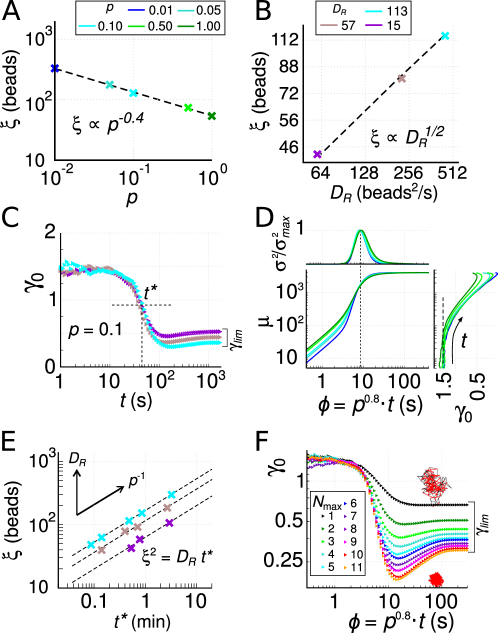
Figure 2: Dependence of the transition dynamics on the kinetic parameters (simulation) (A) Variation of the pearling length $\xi$ with the crosslink probability $p$. (B) Variation of the pearling length $\xi$ with the Rouse coefficient $D_{R}$. (C) Time evolution of $\gamma_{0}$ at different $D_{R}$, Eq. 27 at fixed $p=0.1$. (D) (Lower panel) Mean cumulative number $\mu$ of crosslink events and (Upper panel) its normalized variance $\sigma^{2}/\sigma^{2}_{max}$ as a function of $\phi$, and (Right panel) scatterplot of $\mu$ and $\gamma_{0}$. (E) Scatter plot of the pearling length $\xi$ and the transition time $t^{*}$; dashed lines are plotted using Eq. 8. (F) Evolution of $\gamma_{0}$ as a function of $\phi$ for different values of the monomer functionality $N_{max}$.

The length $\xi$ scales with the crosslink probability $p$ as $\xi\propto p^{-\delta}$, with $\delta=0.4$ (Fig. 2A), indicating that the extent along the chain of the crosslink-induced collapse is paradoxically more prominent for small $p$, i.e. low crosslinking rate. Indeed, conformation changes of polymer loops of size greater than $\xi$ are diffusion-limited, while for smaller loops, Rouse diffusion is faster than the crosslinking reaction. In this latter reaction-limited regime, many conformational fluctuations and contacts can occur and be fixed by crosslinks, producing pearls of mean size $\xi$. Based on this qualitative picture, we propose a mean-field calculation of the dependence of $\xi$ in $p$. The relaxation time for a fixed loop of size $s$ scales as:

$$\tau_{R}(s)=D_{R}^{-1}\cdot s^{2},\ \ \ \mathrm{with}\ \ \ D_{R}=\frac{\pi^{3}}{4}\left(\frac{C_{t}}{C_{s}}\right)^{2},$$ (3)

(detailed derivation in SM §II.E.4) while the average duration $\tau_{cross}$ needed to crosslink contacting beads is inversely proportional to the crosslink probability:

$$\tau_{cross}\propto p^{-1}.$$ (4)

Writing that the pearling length $\xi$ emerges from the competition between these two dynamical processes yields:

$$\xi(p)\propto p^{-\delta},$$ (5)

with $\delta=1/2$ correctly recapitulating the decrease of $\xi$ at increasing $p$. We here assumed that the dynamics is consistent with Rouse diffusion during the pearling formation and collapse. However, Rouse diffusion is not expected to apply to the mesh into what the initially linear polymer is transformed after enough crosslinks, which may explain the different value $\delta=0.4$ measured in the simulations (Fig. 2A). With the same argument we also predict that $\xi$ varies with the dynamical properties of the polymer. Simulations actually show that variation of the Rouse diffusion coefficient $D_{R}$ has a dramatic effect on $\xi$ (Fig. LABEL:fig:sim1B). For small $D_{R}$, $\xi$ is small and crosslinking has mostly a local effect. When $D_{R}$ increases, longer polymer segments can reach their equilibrium conformation between two crosslink events so that $\xi$ becomes larger. In the line of the above calculation, we expect a scaling

$$\xi(D_{R})\propto D_{R}^{1/2},$$ (6)

which is well reproduced in the simulations (Fig. 2B).

Our simulation moreover shows that the collapse happens abruptly. The short-distance exponent $\gamma_{0}$ presents a sharp decrease at a time $t^{*}$, which we call the pearling time. Before this transition ($t\ll t^{*}$), $\gamma_{0}$ coincides with the exponent at long distances, ${3/2}$, as expected for an equilibrium state. Only after the transition a smaller exponent is observed, with a limiting value $\gamma_{lim}<1$ depending on the kinetic parameters. $t^{*}$ depends on the crosslink probability with a scaling $t^{*}\propto p^{-0.8}$ prompting to define a re-scaled variable $\phi=p^{0.8}\cdot t$. The evolution of $\gamma_{0}$ as a function of $\phi$ re-scales at any $p$ into a single transition curve (Fig. 1B). The scaling of $t^{*}$ can also be explained with the above mean-field argument: as $t^{*}$ emerges from pearling (see polymer snapshots along the transition curve in Fig. 1B), it is equal to the relaxation time of pearls of mean size $\xi$: $t^{*}=\tau_{R}(\xi)$. From Eq. 27,

$$t^{*}\propto p^{-2\delta},$$ (7)

and $\phi^{*}=p^{2\delta}\cdot t$. As predicted by the above argument and confirmed in the simulation, the transition time does not depend on the Rouse diffusion coefficient $D_{R}$ (Fig. 2C). The pearling transition is the result of the cooperative effect of multiple crosslinks, that takes place only after relaxation of loops with length $s<\xi$. This effect is highlighted in Fig. 2D, lower panel, that shows the acceleration of crosslink events at the transition. This process is accompanied by the decrease of $\gamma_{0}$ (2D, right panel) and a large increase of crosslink number variability, due to the fluctuation in the size and time of pearl formation and consistent with a phase transition (2D, upper panel). Collecting the results from simulations performed at various values of crosslink probability $p$ and Rouse diffusion coefficient $D_{R}$, the transition points in the plane defined by pearling time $t^{*}$ and pearling length $\xi$ (Fig. 2E) satisfy the Rouse scaling relation:

$$t^{*}=D_{R}^{-1}\cdot\xi^{2};$$ (8)

that fully recapitulates the relationship between these physical quantities. We finally determine the influence of steric constraints on the final state by changing the monomer functionality $N_{max}$. While $\xi$ and $t^{*}$ do not depend on $N_{max}$, the pearl formation and final internal conformation do, as shown by the time behavior of $\gamma_{0}$. After a transition in $t^{*}$, this short-distance exponent transiently goes toward $0$ for large enough values of $N_{max}$ before plateauing to an asymptotic value $\gamma_{lim}$ varying from $0.3$ to $0.7$ when $N_{max}$ varies (see Fig. 2F and Suppl. Fig. 6). Examination of the conformational trajectories shows that this behavior can be explained by a two-stage dynamics taking place after the transition in $t^{*}$. The first stage is the formation of densely connected pearls (in red on the snapshots of Fig. 1A) linked by stretched linkers containing fewer monomers. In these pearls, virtually any monomer can contact any other monomer and $\gamma_{0}$ strongly decreases. A slower process then kicks in: the diffusion-limited crumpling of the stretched linkers between adjacent pearls (see the snapshots in Fig. 2F). In the stretched linkers, mostly adjacent monomers are able to come into proximity, hence the contribution of this collapse to $P(s)$ is such that $\gamma_{0}$ mildly increases.

In summary, our simulation has shown how the interplay between the polymer Rouse dynamics and the rate at which crosslinks are made induces a cooperative phase transition to pearled conformations with characteristic scale $\xi$. We thus obtained a two-stage pearling kinetics, what has already been described in the literature, however with some significant differences in the underlying mechanisms. Our irreversible scenario is not compatible with a simple nucleation and growth process: in the nucleation-inspired model of Buguin et al. (Buguin et al., 1996) pearls created with a minimal size of $\xi$ grow continuously until the overall polymer collapse. We can also exclude knotting effects: Grosberg et al. (Grosberg et al., 1988) focused on the role of knots in the conformational relaxation and predicted a dense globule with a fractal dimension of 3 and a relaxation through reptation. In contrast, we neglect volume interactions which are a necessary element for knot stability. To see whether the appearance of a specific length scale depends on the fact that we used phantom chain, we performed to extra simulation taking explicitly into account steric effect. We found in this case that the pearling dynamics of the transition is unchanged (see Suppl. Fig. 7). We also recovered the local formation of a crumple globule-like state in each pearl with $\gamma_{0}=1$. The emergence of the characteristic length $\xi$ however excludes fractality of the absorbing conformations. The scale-dependent behavior observed in our simulation reflects the presence of two different dynamics: reaction-limited pearling at short distances along the chain, diffusion-limited collapse at large distances.

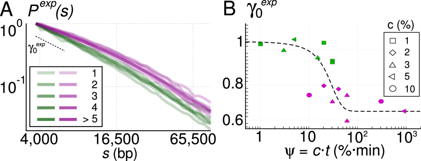
Figure 3: (A) Experimental contact probability curves $P^{exp}(s)$ for various crosslinker concentrations $c$, displayed as a superposition of semitransparent plots (see Fig. 1A). (B) Evolution of the experimental slope $\gamma_{0}^{exp}$ as a function of the re-scaled time variable $\psi=c\cdot t$ (see Fig. 1B). The color discriminates the experiments belonging to the two modalities for $\gamma_{0}^{exp}$, the dashed line is a guide for the eyes.

Experimental approaches in chromosome biology have been recently renewed by chromosome conformation capture (3C) that uses a succession of crosslinking, restriction, religation and sequencing steps to measure contact frequencies along a DNA molecule in vivo. This technique centrally exploits the unique opportunity offered by the DNA heteropolymer to have a single sequence identifier at each loci (for long enough identifiers) and so to derive a contact probability curve $P(s)$ from crosslink counts. In the seminal paper introducing the genome-wide 3C technique, Hi-C, Lieberman-Aiden et al.  (Lieberman-Aiden et al., 2009) fitted the resulting curve with a scaling relation $P(s)\propto s^{-\gamma}$, in the range between 1 and 10 millions base pairs (bp), with a value of $\gamma$ close to $1$ compatible with a fractal-globule state. However, an exponent of $0.75$ has also been reported at shorter scale, and other out-of-equilibrium mechanisms were invoked to explain this alternative exponent: the tension globule (Sanborn et al., 2015) or the extrusion of loops by molecular motors such as condensins  (Sanborn et al., 2015; Fudenberg et al., 2016). While these mechanisms can have a role in chromosome folding, the models do not take explicitly into account the potential distortion that the DNA polymer can undergo during the initial step of the experiment, consisting in chemically crosslinking DNA with formaldehyde. This crosslinking step prompted us to exploit this experimental technique to check the collapse scenario described in our simulations.

In order to start from configurations that are the closest possible to a simple homopolymer, we used synchronized yeast cells that are neither replicating nor dividing. We performed Hi-C (methods in SM §I.D and (Cournac et al., 2012; Lazar-Stefanita et al., 2017)) at different formaldehyde concentrations $c$ and exposure times $t$ in order to observe the evolution of polymer conformations during the crosslink-induced collapse. Not knowing the reaction order, we cannot establish an exact mapping between $k_{on}$ and $c$, so we used a simple ansatz, $\psi=c\cdot t$, for the re-scaled time variable. The experimental curves $P^{exp}(s)$ cluster around two different mean-curves differing by their slope at short distances $\gamma_{0}^{exp}$ (Fig. 3A). Plotting this exponent as a function of $\psi$, we observe a sharp transition (Fig. 3B) as predicted by the simulations. Two differences are nevertheless worth discussing. Before the transition, the short-distance exponent of yeast chromosomes is not equal to $1.5$ as in simulations (Fig. 1B), but to $1$ ($0.05\;s.d.$). This value might either correspond to an effect of volume interactions during the early phases of pearling collapse or to an in-vivo special organization of the DNA in chromosomes, potentially induced by the regular wrapping of DNA around the nucleosomal protein spools. For distances above 10 kb these constraints weaken and the chain follows a more typical random walk with an exponent closer to $1.5$. After transition, $\gamma_{0}^{exp}$ equals to $0.7$ ($0.06\;s.d.$), corresponding to the value observed for $N_{max}=1$ in simulations. This value is likely explained by strong steric constraints preventing a crosslinked locus to contact other loci. The precise estimation of $\xi$ was impaired by the higher biological, experimental and statistical noise on $P^{exp}(s)$ at increasing distance $s$, so that we could not measure experimentally the dependency of $\xi$ on the crosslinker concentration. Nevertheless, the experiment clearly demonstrate that a polymer experiencing a crosslink-induced collapse undergoes a sudden transition. It also confirms that inside pearls, at length scales lower than $\xi$, the polymer conformation in the absorbing asymptotic state is very compact, with an exponent $\gamma_{0}$ lower than $1$, whereas the polymer topology remains unchanged at longer length scales.

We thank Madan Rao, John Marko, Jean-Marc Victor, Benjamin Audit, Marco Cosentino-Lagomarsino, Maxim Dolgushev and Daniel Jost for the extremely useful discussions and suggestions, and Véronique Legrand and the DSI of Institut Pasteur for the computational power and assistance.

Supplementary Materials

I Methods

I.1 Simulation method

I.1.1 Source code

The code for reproducing the simulations contained in this manuscript is available on GitHub at https://github.com/scovit/crosslink and is compatible with the Linux operating system. Compilation requires a recent version of gcc, GNU make, OpenGL, OpenSSL, flex and bison and can be achieved by the command make. Hardware requirements include a recent x86-64 CPU with supports for the AVX instruction set. After compiling, the code can be run with the command ./crosslink[.gl] configuration.info. Sample configuration files are provided in the samples folder and the optional extension .gl activates the real-time graphical visualization of the simulation.

I.1.2 Algorithm description

We simulate the crosslinking process under the minimal assumptions that (1) chromosomes are ideal chains of monomers and (2) the effect of crosslinking is an irreversible topological change between distant monomers on the chain. We model a chromosome as a $2048$ beads polymer fluctuating in three dimensional space using a variant of the off-lattice bead-spring Monte-Carlo (MC) algorithm described in refs. cacciuto2006self, scolari2015combined. Each bead of the polymer represents a group of $3$ nucleosomes, or $500$ base pairs (as in ref. hajjoul2013high), adjacent beads are linked by an infinite spherical potential of radius $b$, thus forbidding any dynamical moves which would settle them at larger distances while allowing everything else, each MC move selects randomly a single bead and attempts a move in a random direction uniformly, normally sampling a sphere of radius $0.6\cdot b$. Different mean-square displacements (MSD) for a bead have been obtained by varying the size of the random move from $0.066\cdot b$ to $0.2\cdot b$.

We used the value of $b=24$nm, which is an estimation of the maximum distance that can be covered by three fully stretched nucleosomes, and one MC sweep as $6.7\cdot 10^{-4}\,$secs, estimated by fitting the motility of the tracking dynamics of single loci hajjoul2013high, see next section for details.

After a fixed thermalization time $t_{0}$, the crosslinking process is introduced in the simulation as an irreversible and configuration-dependent change in the chain topology. After each accepted MC move, if a couple of beads are found at a distance lower than $r_{int}=b/64$ units a link is introduced with a given probability $p$ that we consider as a proxy for the crosslinker concentration $c$, and the couple is added to the list of adjacent beads. Crosslinks are totally irreversible, and a maximum number of crosslinks $N_{max}$ for each bead is allowed, mimicking steric effects. When it is not otherwise specified, $N_{max}$ is taken equal to 4. Such events are then counted as contacts and mean contacts maps are built by summing all the contacts over a population of independently simulated chains.

I.1.3 Reproduction of the polymer equilibrium dynamics

The simulation integrates the stochastic Rouse dynamics as an effective model using a purely entropic dynamical Monte-Carlo (MC) algorithm. This section details the reproduction of Rouse dynamical features using the simulated dynamics. Rouse Dynamics predicts two power-law behaviors: (1) the trajectory of a polymer unit segment (monomer) displays a mean square displacement (MSD) scaling with time with a sub-diffusive exponent $1/2$, and (2) at any fixed time, the conformation of the polymer displays a mean square distance scaling with the backbone distance with an exponent $1$. The coefficients $C_{t}$ and $C_{s}$ are defined from these scaling behaviors according to:

$$\left\langle\left|\vec{R}(s,t_{0})-\vec{R}(s,t+t_{0})\right|^{2}\right\rangle=C_{t}\cdot t^{1/2}\quad\mathrm{and}\quad\left\langle\left|\vec{R}(s_{0},t)-\vec{R}(s+s_{0},t)\right|^{2}\right\rangle=C_{s}\cdot s,$$ (9)

where $\vec{R}(s,t)$ is the location at time $t$ of the monomer at position $s$ along the polymer chain, $\langle\cdot\rangle$ is the mean over a population/ensemble of chains, $t_{0}$ and $t+t_{0}$ are two observation times, and $s_{0}$ and $s+s_{0}$ are two genomic coordinates; for details and derivations see doi1988theory and Appendix, seq:relaxexac. In the experimental situation we considered, measurements of in-vivo Yeast chromatin reported the validity of both scaling behaviors bystricky2004long, hajjoul2013high, and provide a direct measurement of the two parameters $C_{t}$ and $C_{s}$ characterizing the equilibrium dynamics of the system.

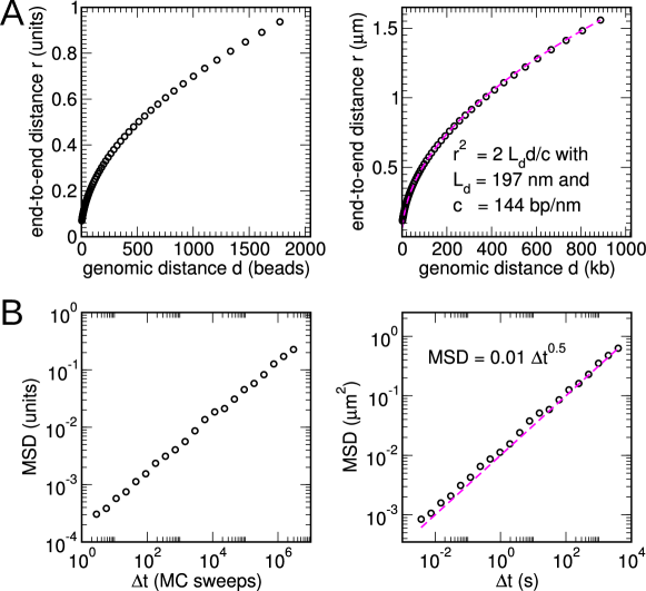
Suppl. figure 1: Rouse dynamics and reproduction by the simulated dynamics of published experimental coefficients: (A) measurement of the end-to-end distance as a function of the genomic distance at equilibrium; the left panel displays the numerical data from simulations, the right panel displays the data rescaled to fit with the observed coefficient $C_{s}=2\cdot 197/144\ {\rm nm^{2}/bp}$, adapted from (B) The unit of measure for time (s) has been defined by fitting the coefficient of power-law describing the MSD as a function of time with the observed motility coefficient $C_{t}=0.01{\rm\mu m^{2}/s^{1.2}}$, adapted from

It is possible to assign units of time ($sec$) and space ($nm$) to simulated quantities by relating the numerical coefficient $C_{t}$ and $C_{s}$ in the simulations and their values in the experimental results. The proof of concept is presented in Suppl. fig:fittone, demonstrating that it is possible to fit the experimentally measured behaviors and associated coefficients with those observed in the simulation. While this approach could allow us to fix the values of the biophysical units using the most up-to-date literature, we acknowledge that this approach presents the flaw that those two parameters depends on the experimental conditions and scale, see grosberg2016scale and Appendix, seq:relaxexac. Depending on the experimental conditions, the scale value can correspond to totally different microscopical quantities, namely it can depend on the size of the fluorescent locus during optical measurements javer2013short, the length of the DNA-linkers between nucleosomes in in-vitro experiments bednar1998nucleosomes, kornberg1977structure, a characteristic length dependent on the local density of monomers if the excluded-volume is predominant wyart2000viscosity, brochard1979conformations, a characteristic time dependent on active noise fluctuations in dynamical measurements weber2012nonthermal, osmanovic2017dynamics, or other constraints and microscopical properties of the chromatin, for instance weber2010bacterial, amitai2013polymer. Additionally, some of these elements weber2010bacterial, amitai2013polymer, weber2012nonthermal, osmanovic2017dynamics, as well as strong steric marenduzzo2006entropy and hydrodynamic doi1988theory effects, can alter the scaling behaviors of (9). The two experiments reproduced in Suppl. fig:fittone (bystricky2004long, hajjoul2013high) display a robust scaling, but are not made in identical controlled environments. As such, we decided to fix the simulation spatial unit through a definition of the maximum extension of linkers between three nucleosomes $b=24$nm and, after, to fit the temporal scaling behavior of MSD as in Suppl. fig:fittoneB for the definition of the unit of time.

To obtain Suppl. fig:fittone, the end-to-end distance as a function of the genomic distance, we measured the equilibrium conformation along time of 64 parallel polymer simulations, then calculated the mean distance in function of genomic distance and log-binned the data though a geometric progression of ratio of 2. To obtain the MSD as a function of time, we collected for the same 64 parallel equilibrium simulations the trajectories of the bead placed in the center of the polymer chain; then we subtracted from each trajectory the position at time zero and we calculated the square of each three-dimensional vector and log-binned the resulting curve through a geometric progression or ratio of 2.

I.1.4 Irreversible crosslinking process

The simulation implements Rouse dynamics with the addition of crosslinks, namely irreversible and configuration-dependent changes in the chain topology. In detail, after each accepted MC move, in case a couple of beads are found at a distance lower than $r_{int}=b/64$ units, a crosslink is introduced between them with a given probability $p$ that we consider as a proxy for the crosslinker concentration $c$ and the couple is added to the list of adjacent beads (in the 3D space). This section reconsiders this proxy connecting the parameter $p$ to physico-chemical quantities.

The problem of irreversible reactions can be restated as a first passage-time problem: in the most basic examples (e.g. the decay radioactive atomic nuclei), the on-rate of transition from state A to state B is a constant in time, which is called $K_{on}$. As such, considering a finite (continuous) amount of time $\Delta t$, the probability $p$ of passing from A to B in that amount of time can be calculated from the rate of doing the transition integrated over the elapsed time

$$p=1-e^{-K_{on}\Delta t}.$$ (10)

The general problem of polymer crosslinking reaction is more complex because at least two concurrent processes are contributing to the probability of making a crosslink: (1) the diffusion of the polymer is creating three-dimensional contacts, that is a necessary condition for the reaction to happen and (2) the reaction of the crosslinking agent with proteins and then with DNA fixes the contacts defined that way. The first process is simulated by the Rouse dynamics described in the previous section, i.e. contacts get continually activated and dissolved depending on the polymer parameters and the genomic distance. The second process, described in chemical details in Hoffman et al. hoffman2015formaldehyde, is, in our simulations, considered as an irreversible transition parameterized by a single parameter $p$ depending on crosslinker concentration and phenomenologically modeling the detailed description.

A study of the simple function in (10) reveals that if $\Delta t$ is small ($\Delta t\ll 1/K_{on}$), then the dependency between the probability $p$, the rate $K_{on}$ and time $\Delta t$ can be approximated by this linear relation: $p\simeq K_{on}\Delta t$. Since the distribution of $\Delta t$ in our simulations is short-tailed (see Suppl. fig:difflimB), we can take its mean as a value for $\Delta t$ in (10), connecting the parameter $K_{on}$ with the dimension of a rate (inverse of a time) to a crosslink probability $p$. The results of this approach are valid as long as the simulation is in this reaction-limited regime ($K_{on}\ll 1/\Delta t$ such that $p\ll 1$) at the lowest spatial scales.

Regarding the connection between $K_{on}$ and the crosslinker concentration $c$, the emergence of a single experimental collapse curve for the exponent $\gamma_{0}$ when it is considered as a function of the rescaled time variable $\psi=c\cdot t$ (see figure 4B, main text) suggests that the transition rate $K_{on}$ depends linearly on the concentration, although from this single experiment, we cannot exclude reaction orders smaller than 3. From the biophysical point of view, the dimensionless values of $p$ from simulations could be related quantitatively to experiments once a precise quantitative measurement of the reaction order and a quantitative measurement of the typical contact duration $\Delta t$ would have been performed.

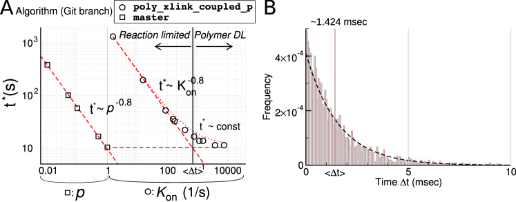
Suppl. figure 2: Transition between reaction-limited to diffusion-limited crosslinking dynamics: (A) Results from simulations using the poly_xlink_coupled_p algorithm (circles) show a scaling relationship with exponent $0.8$ between the transition time $t^{*}$ and the association constant $K_{on}$ in the reaction-limited regime (dashed red lines); they also evidence the transition for $\langle\Delta t\rangle\gg 1/K_{on}$ to a polymer diffusion-limited regime (DL). Results from simulations using the master algorithm (boxes) display a similar scaling in the reaction-limited regime upon rescaling $K_{on}$ by the transition value $\langle\Delta t\rangle^{-1}$. (B) The distribution of the duration $\Delta t$ of contacts in our algorithms depends on the Rouse chain parameters $C_{t}$ and $C_{s}$, and it might depend on additional biophysical constraints in experiments. The histogram presented here has been obtained with the same parameters as those used in the main text.

An alternative, but more complex, approach (code available in the poly_xlink_coupled_p branch in GitHub) to relate the crosslinking dynamics to the polymer dynamics, consists in having the simulation keeping track of the time a contact has been created, and, at the time when the contact is released, calculate the probability of having made a crosslink during that time as the discrete version of (10) above: $p=1-(1-k_{on})^{\Delta t}$ where $\Delta t$ is the discrete elapsed time expressed in terms of number of MC steps and $k_{on}$ is a dimensionless rate; then, according to a uniform sampling, decide if a crosslink has been made or not. A study of the results reveals the presence of a transition between a reaction-limited regime and a polymer-diffusion-limited regime: if $\Delta t$ is small ($\Delta t\ll 1/k_{on}$), then the system is in a reaction-limited regime, and the dependency between the probability $p$, the rate $k_{on}$ and time $\Delta t$ can be approximated by this linear relation: $p\simeq k_{on}\Delta t$. For larger $\Delta t$, the probability is instead equal to $p\simeq 1$, and the crosslink reaction becomes only polymer-diffusion-limited. We plotted the transition curve for $\gamma_{0}$ with this algorithm and show the presence of the two distinct behaviors for the dependency of the transition time on $k_{on}$: a power law with exponent $0.8$ in the reaction-limited regime (see main text) and no dependency on $k_{on}$ in the diffusion-limited regime (see Supplementary fig:difflimA, circles). The results, apart from a rescaling, are similar to the results of the simpler algorithm (Supplementary fig:difflimA, squares).

Finally, we speculate that taking into account the transition from diffusion-limited to reaction-limited regimes, the expressions for pearling size $\xi$ and time $t^{*}$ will be (denoting $\xi_{cr}$ and $t^{*}_{cr}$ the pearling size and time for $p=1$):

$$\begin{split}&\frac{t^{*}-t^{*}_{cr}}{t^{*}_{cr}}=p^{-2\delta},\ \ \ \mathrm{and}\\ &\frac{\xi-\xi_{cr}}{{t^{*}_{cr}}^{1/2}}=D_{R}^{1/2}p^{-\delta},\ \ \ \mathrm{with}\\ &\xi_{cr}^{2}=D_{R}\cdot t^{*}_{cr}\ \mathrm{and}\ \delta=0.4;\end{split}$$ (11)

which model the crossover. Equation (LABEL:*)eq:xit2 resumes equations 5, 6, 7 and 8 from the main text. They display explicitly the dependency on the crosslink probability $p$, introduce a soft crossover toward the critical value $p=1$ and the bounds $\xi_{cr}$ and $t^{*}_{cr}$ to be determined experimentally.

I.2 Simulation data analysis

I.2.1 Generation of contact matrices

For each set of parameters, simulations has been launched in batches of 2000 identical runs on the TARS cluster of “Pasteur Institut”, powered by 3500 identical CPUs. Time and information about the couple of involved beads have been recorded for each crosslinking event for each parallel simulation in distinct data-files. Sparse matrices have been generated, merging all batches, summing the number of crosslinking events happening for each couple of beads up to a specified time. Time has been sampled according to a geometric progression of initial value and common ratio equal to $1.1$, discarding all matrices with less than $512$ contacts. Contact matrices for ideal polymer models at very long time (after the transition) at various crosslinking probabilities look like the one reported in Suppl. fig:contmat.

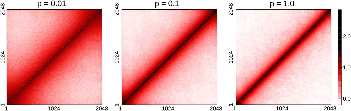
Suppl. figure 3: Contact matrices for ideal polymer models (simulation) at very long time (after the transition) at various crosslinking probabilities

I.2.2 Calculation of $P(s)$ in the simulation

In the simulation, sparse matrices have been coarse-grained to bead-level dense matrices. Binning of the contact probability $P(s)$ at bead level has been made by calculating the mean value of secondary diagonals for $s$ varying in the range from 1 to 2048 beads. In order to reduce the noise level at large linear distances $s$ (along the polymer chain) and avoid the effect of chain discretization at small distances, the curve $P(s)$ has been binned according to the following scheme: values for $s$ less then $5,000$bp were discarded; then binning has been performed at single bead level (bins of $500$bp) for distances $s$ less than $10,000$bp, then we used bins of $1,000$bp for $s$ between $10,000$ and $20,000$bp, bins of $2,000$bp for $s$ between $20,000$ and $40,000$bp, and finally bin sizes defined according to a geometric progression (log-binned) of initial value and common ration equal to $1.1$ for distances $s$ greater than $40,000$bp. The contact distribution is obtained as the weighted histogram computed from the sum of read pairs for each bin, weighted with the expected number of pairs under the uniform null hypothesis, which takes into consideration the bin size. To compare different conditions, distributions were normalized by the value of their first bin, yielding contact probability curves $P(s)$.

I.2.3 Determination of the collapse transition

The local slope $\gamma(s)$ along the chain, at a linear distance $s$, has been calculated by performing a linear regression on a sliding-window on the log-log plot of the $P(s)$, using a window of size equal to 7 data-points. The collapse transition has been determined by collecting, for each simulation condition, the slope $\gamma$ of the linear regression performed on the first 7 data-points falling in the interval of $s$ values between $5,000$ and $8,500$ bp.

I.2.4 Determination of the transition values $t^{*}$ and $\xi$

The pearling size $\xi$ has been measured on the local slope $\gamma(s)$ as a function of the linear distance $s$ by measuring the first value $s$ for which $\gamma(s)>0.9$. The transition time $t^{*}$ (pearling time) has been measured as the first value of time $t$ for which $\gamma_{0}>0.9$.

I.2.5 Determination of the Rouse coefficient from MSD scaling

The Rouse coefficient, $D_{R}$, has been calculated in the simulation from the measured prefactor, $C_{t}$, in the scaling of the MSD as a function of time and the effective persistence length, $C_{s}$, through the formula (see Suppl. Methods sec:repeq)

$$D_{R}=\frac{\pi^{3}}{4}\left(\frac{C_{t}}{C_{s}}\right)^{2},$$ (12)

see Appendix sec:relaxexact for the derivation.

I.3 Generation of Hi-C data-sets

I.3.1 Crosslink conditions on G1 elutriated cells

S. cerevisiae [BY4741] cells were inoculated and for $8\text{\,}\mathrm{h}$ in $10\text{\,}\mathrm{mL}$ YPD, then $500\text{\,}\mathrm{\SIUnitSymbolMicro L}$ of the pre-culture were inoculated and grown overnight in $500\text{\,}\mathrm{mL}$ YPD. $500\text{\,}\mathrm{mL}$ overnight culture was centrifuged and pelleted, then cells were resuspended in $500\text{\,}\mathrm{mL}$ of fresh YPD for $3\text{\,}\mathrm{h}$ at $30\text{\,}\mathrm{\SIUnitSymbolCelsius}$. G1 daughter cells were recovered from this exponentially growing population through an elutriation procedure marbouty2014purification. Before fixation, G1 cells were refreshed in $150\text{\,}\mathrm{mL}$ of fresh YPD at $30\text{\,}\mathrm{\SIUnitSymbolCelsius}$ for $30\text{\,}\mathrm{min}$ ($2.5\times 109$ G1 cells/fraction). Cells were crosslink using formaldehyde (Sigma) under different conditions of concentration and time (see Suppl. Table 1). The crosslink reaction was quenched with $25\text{\,}\mathrm{mL}$ glycine $2.5\text{\,}\mathrm{\textsc{m}}$ for $20\text{\,}\mathrm{min}$ at $4\text{\,}\mathrm{\SIUnitSymbolCelsius}$. Crosslinked cells were recovered through centrifugation, washed with YPD, pelleted and stored at $-80\text{\,}\mathrm{\SIUnitSymbolCelsius}$ into $2\text{\,}\mathrm{mL}$ centrifugal tube.

I.3.2 Generation of Hi-C libraries

Hi-C libraries were generated as described in dekker2002capturing, cournac2016generation with introduction of a biotin-ligation step in the protocol lieberman2009comprehensive. To generate the libraries, a pellet of G1 cells, previously crosslinked, was thawed on ice. Then, the cells were incubated for $30\text{\,}\mathrm{min}$ in $10\text{\,}\mathrm{mL}$ of sorbitol $1\text{\,}\mathrm{\textsc{m}}$ with DTT $5\text{\,}\mathrm{m}\mathrm{\textsc{m}}$ and Zymolyase 100T (CFinal = $1\text{\,}\mathrm{m}\mathrm{g}\mathrm{/}\mathrm{m}\mathrm{L}$) to digest the cell wall. Spheroplasts were then washed first with $5\text{\,}\mathrm{mL}$ of sorbitol $1\text{\,}\mathrm{\textsc{m}}$, then with $5\text{\,}\mathrm{mL}$ of 1X restriction buffer (depending on the restriction enzyme used). Spheroplasts were washed with $5\text{\,}\mathrm{mL}$ sorbitol $1\text{\,}\mathrm{\textsc{m}}$, then with $5\text{\,}\mathrm{mL}$ 1X restriction buffer (NEB), and suspended in $3.5\text{\,}\mathrm{mL}$ 1X restriction buffer. Cells were split into aliquots (V = $500\text{\,}\mathrm{\SIUnitSymbolMicro L}$) and incubated in SDS (3%) for $20\text{\,}\mathrm{min}$ at $65\text{\,}\mathrm{\SIUnitSymbolCelsius}$. Crosslinked DNA was digested at $37\text{\,}\mathrm{\SIUnitSymbolCelsius}$ overnight with 150 units of DpnII restriction enzyme (NEB). The digestion mix was subsequently centrifuged for $20\text{\,}\mathrm{min}$ at 18,000 g and the supernatant discarded. Pellets were suspended in cold water. DNA ends were repaired in the presence of 14-dCTP biotin (Invitrogen), and crosslinked complexes incubated for $4\text{\,}\mathrm{h}$ at $16\text{\,}\mathrm{\SIUnitSymbolCelsius}$ in presence of 250 U of T4 DNA ligase (Thermo Scientific, $12.5\text{\,}\mathrm{mL}$ final volume). DNA purification was achieved through an overnight incubation at $65\text{\,}\mathrm{\SIUnitSymbolCelsius}$ with $250\text{\,}\mathrm{\SIUnitSymbolMicro}\mathrm{g}\mathrm{/}\mathrm{m}\mathrm{L}$ proteinase K in $6.2\text{\,}\mathrm{m}\mathrm{\textsc{m}}$ EDTA followed by a precipitation step and RNAse treatment. The resulting Hi-C DNA libraries were 500 bp fragmented, using CovarisS220 apparatus. Fragments between 400 and 800 bp were purified and the biotin-labeled fragments were selectively captured by Dynabeads Myone Streptavidin C1 (Invitrogen). Purified fragments were amplified by PE-PCR primers and paired-end sequenced on the NextSeq500 Illumina platforms ($2\times 75$ bp).

I.3.3 Raw data processing

Suppl. tab:xlc contains the information about experimental crosslinking conditions.

strains	crosslink concentration	crosslink time	# reads
BY4741	1 % (V = 4.2 mL)	1 min	9190059
BY4741	1 % (V = 4.2 mL)	20 min	1608139
BY4741	1 % (V = 4.2 mL)	30 min	13693706
BY4741	2 % (V = 8.4 mL)	10 min	3056592
BY4741	2 % (V = 8.4 mL)	20 min	5655336
BY4741	3 % (V = 12.6 mL)	1 min	1977469
BY4741	3 % (V = 12.6 mL)	5 min	1616825
BY4741	3 % (V = 12.6 mL)	10 min	6091165
BY4741	3 % (V = 12.6 mL)	10 min	1630060
BY4741	3 % (V = 12.6 mL)	20 min	1389810
BY4741	3 % (V = 12.6 mL)	20 min	2079929
BY4741	5 % (V = 21 mL)	1 min	2223222
BY4741	5 % (V = 21 mL)	180 min	1143955
BY4741	10 % (V = 42 mL)	1 min	18367276
BY4741	10 % (V = 42 mL)	30 min	17466440

Suppl. table 1: Genomic DNA in living cells was crosslinked using formaldehyde (Sigma) under different conditions of crosslinker concentration and experiment duration

Raw Hi-C data were processed as follows. PCR duplicates were removed using the 6 Ns present on each of the custom-made adapter and the 2 trimmed Ns. Paired-end reads were mapped independently using Bowtie 2.1.0 (mode: --very-sensitive --rdg 500,3 --rfg 500,3) against the S. cerevisiae reference genome (S288C). An iterative alignment, with an increasing truncation length of 20 bp, was used to maximize the yield of valid Hi-C reads (mapping quality $>30$). Only uniquely mapped reads were retained. On the basis of their DpnII restriction fragment assignment and orientation, reads were classified as either valid Hi-C products or unwanted events to be filtered out (i.e., loops, non-digested fragments, etc.); for details see cournac2012normalization, cournac2016generation. The amount of reads in contact maps is reported in table tab:xlc.

I.4 Experimental data analysis

I.4.1 Calculation of $P^{exp}(s)$ from Hi-C data

Pairs of intra-chromosomal reads mapping positions along the genome were partitioned according to chromosomal arms. Reads oriented towards different directions or separated by less than 3 kb were discarded. For each chromosomal arm, except for the right arm of the chromosome XII which comprises the rDNA, read pairs were log-binned according to the genomic distance $s$ separating them (in kb), $bin=\mathrm{floor}[\log_{1.1}(s)]$. The contact probability distribution $P^{exp}(s)$ is the histogram computed from the sum of read pairs for each bin, locally normalized by the expected number of pairs in this bin under the uniform null hypothesis. To compare different conditions, distributions were globally normalized by the value of their first bin. Sample experimental contact matrices before and after the transition are reported in Suppl. fig:expmat.

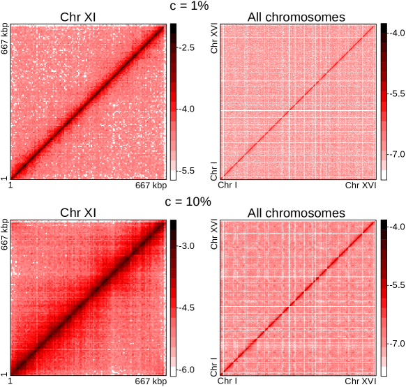
Suppl. figure 4: Sample experimental contact matrices before and after the transition

I.4.2 Determination of the collapse transition

The local slope $\gamma^{exp}(s)$ as a function of the genomic distance $s$ has been calculated by performing a linear regression on a sliding-window on the log-log transformation of $P^{exp}(s)$, on a window of the size of 7 data-points. The collapse transition has been built by collecting, for each crosslink concentration and time, the slope coefficient of the linear regression performed on the 7 data-points falling in the $s$ interval between 3,800 bp and 6,150 bp.

II Appendix

II.1 Measurement of pearls with Louvain algorithm

Pearls were detected automatically using the Louvain clustering algorithm blondel2008fast on the contact map of the crosslinked polymer. For two markedly different values of the crosslink probability $p$, we found that the number of monomers per pearl displays a peaked distribution with a mean corresponding closely to the measured value of the pearling length $\xi(p)$ (top panels on the Suppl. fig:louv). We computed the volume of the pearls, either using the radius of gyration $R_{g}$ or the convex hull surrounding each pearl. We found that the volume of the pearls increases with the number on monomers found in each pearl (middle and bottom panels).

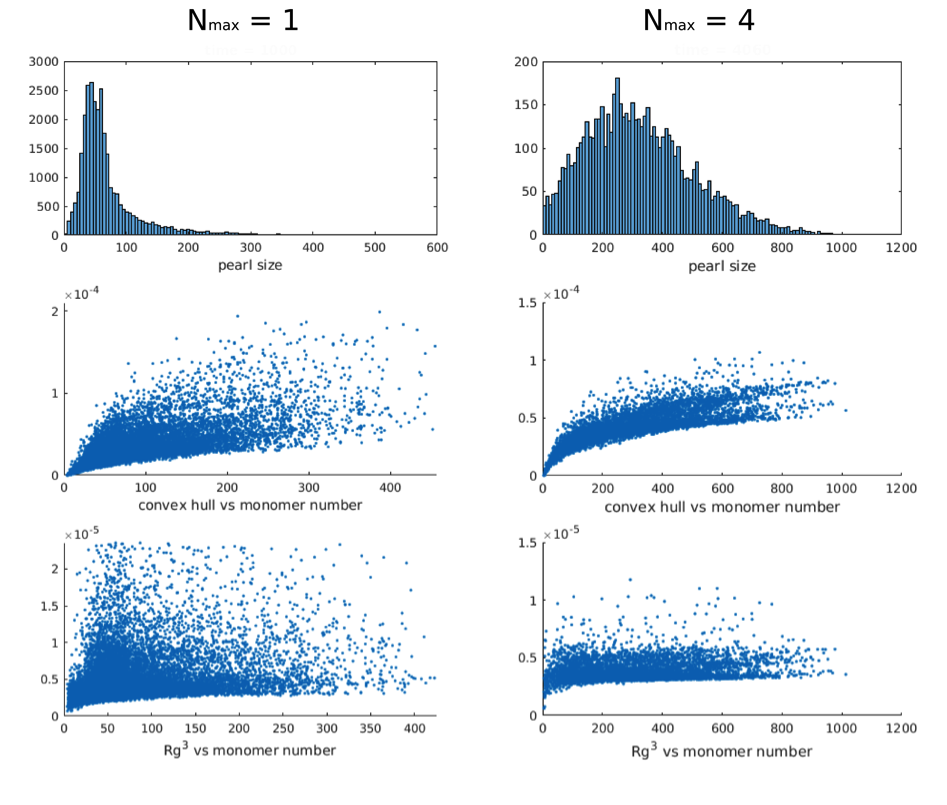
Suppl. figure 5: From top to bottom: distribution of pearl sizes, convex hull in function of number of monomers in the pearl and radius of gyration to the cube in function of number of monomers in the pearl. Left panels are for $p=0.05$ and $N_{max}=1$, right panels for $p=0.1$ and $N_{max}=4$

II.2 Short-scale exponent $\gamma_{lim}$ at the end of fixation ($t\gg t^{*}$)

The measured $\gamma_{0}$ after the pearling transition ($t\gg t^{*}$) is not a constant, but depends on different simulation parameters. For large values of $N_{max}$, $p$ and $D_{R}$, $\gamma_{0}$ dynamically and transiently goes toward 0, before plateauing at final values $\gamma_{lim}$ (see figure 3F, main text). Suppl. Figure 6 highlights the dependence of this value on the relevant dynamical parameters, suggesting a characteristic final phase with fractal properties.

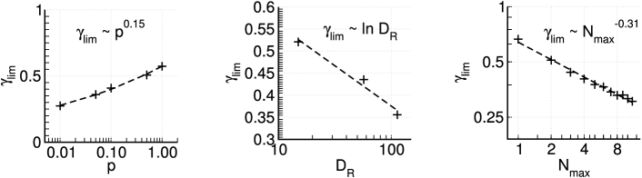
Suppl. figure 6: Dependence of $\gamma_{lim}$ on $p$, $D_{R}$ and $N_{max}$.

II.3 Effects of additional steric interactions

We repeated some simulations for a few sets of parameters (only a few due to heavy computational requirements) taking into account excluded volume. The results, presented below, show that despite the fact that the initial and final values for $\gamma_{0}$ are (as expected) different with excluded-volume, the cooperative effect and the scaling of the dynamics are not significantly modified. Specifically, we included a hard-sphere potential between monomers (beads) whose range matches the average distance between consecutive monomers. This leads to a change in the exponent of the equilibrium contact probability curve $P_{0}(s)$ from -1.5 (random walk) to -2.2 (four-legged polymer-loop exponent, marenduzzo2006entropy). While the initial state of the polymer is different, its collapse follows a dynamics very similar to the phantom-case dynamics described in our manuscript. Interestingly, the final state inside the pearls exhibits an exponent $\gamma_{0}=1$, that could correspond to a crumple globule (also called fractal globule) as originally described by grosberg1988role.

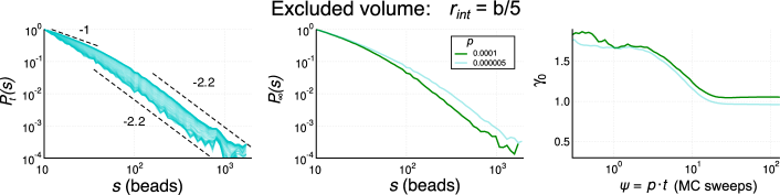
Suppl. figure 7: Result of adding hard-core repulsive interactions, from left to right: 1) the evolution of $P_{t}(s)$ in function of crosslinking time with $p=0.0001$, 2) the adsorbing $P_{\infty}(s)$ at different values of $p$ and 3) the dynamics of $\gamma_{0}$ in function of $t$ at different values of $p$.

II.4 Videos of the simulations

Videos of the simulations are available at the following link:

https://github.com/scovit/crosslink/tree/master/videos
The screen of the video is divided in 4 quadrants, from left to right and top to bottom. The first quadrant show the evolution of the HiC matrix for the single polymer in time; the second quadrant is the video of the polymer simulation where each bead is in red, the third and fourth quadrant show the polymer at the bead level (in grey) superimposed with beads calculated by the center of mass of blocks of respectively 8 and 126 beads, to highlight the different relaxation dynamics at different scales. The video are filmed at real computing time, with parameters $p=1.0$ and $N_{max}=1$.

II.5 Analytical phenomenology of a scale-free Rouse model

II.5.1 The Rouse equation

The Newton equation of motion with viscous friction and random noise for a point particle standing at position $\vec{R}(t)$ at time $t$ is:

$$\begin{split}F^{i}(t)&=m\frac{\partial^{2}R^{i}}{\partial t^{2}}-\zeta\frac{\partial R^{i}}{\partial t}+\eta^{i}(t),\\ \mathrm{with}\ \langle\eta^{i}_{n}(t)\rangle=0&\ \ \ \mathrm{and}\ \ \ \langle\eta^{i}_{n}(t)\eta^{j}_{n^{\prime}}(t^{\prime})\rangle=2\zeta k_{B}T\delta^{ij}\delta_{nn^{\prime}}\delta(t-t^{\prime})\end{split}$$ (13)

In overdamped conditions we can drop the inertial term $m\frac{\partial^{2}R^{i}}{\partial t^{2}}\simeq 0$. For a system of many particles, in the absence of external forces and when the point particle (a bead) belongs to a Gaussian-potential chain (linking the bead indexed by $n$ with $n-1$ and $n+1$) of Young modulus $K$, we get the stochastic equation for the free discrete polymer, also called the Rouse equation:

$$\begin{split}\zeta\frac{\partial R^{i}_{n}(t)}{\partial t}=K\left[R^{i}_{n+1}(t)+R^{i}_{n-1}(t)-2R^{i}_{n}(t)\right]+\eta^{i}_{n}(t),\\ \mathrm{with}\ \langle\eta^{i}_{n}(t)\rangle=0\ \mathrm{and}\ \langle\eta^{i}_{n}(t)\eta^{j}_{n^{\prime}}(t^{\prime})\rangle=2\zeta k_{B}T\delta^{ij}\delta_{nn^{\prime}}\delta(t-t^{\prime})\end{split}$$ (14)

II.5.2 Scaling laws and relaxation times

Considering the polymer chain as a continuous and infinite succession of segments of infinitesimal length fluctuating in the three-dimensional space in over-damped conditions (no inertial contributions) under the influence of random forces, the discrete stochastic (14) can be approximated by:

$$\zeta\frac{\partial R^{i}(n,t)}{\partial t}=K\frac{\partial^{2}R^{i}(n,t)}{\partial n^{2}}+\eta^{i}(n,t),$$ (15)

where $R^{i}(n,t)$ is the $i$-th component of the position corresponding the $n$-th internal degree of freedom at time $t$; $\zeta$ and $K$ are parameters (possibly temperature-dependent) with dimension of friction and energy, respectively, and not necessarily equal to the solvent parameters as measured by bead probes.

We can use the Fourier transformation, basically passing to the conjugate variable $p$ through the identities:

$$\tilde{R}^{i}(p,t)=\frac{1}{\sqrt{2\pi}L}\int_{\mathbb{R}}\!\mathrm{d}n\,e^{-i2\pi pn}\,R^{i}(n,t),\ \ \mathrm{and}\ \ R^{i}(n,t)=\frac{L}{\sqrt{2\pi}}\int_{\mathbb{R}}\!\mathrm{d}p\,e^{i2\pi pn}\,\tilde{R}^{i}(p,t)$$ (16)

$L$ represents the value of the Dirac delta in zero: $\left.\delta(p)\right|_{p=0}=L$ and $\left.\delta(n)\right|_{n=0}=L^{-1}$. It can be formally interpreted through a limit-integral representation of the delta function in term of box functions, and it can in fact be chosen arbitrarily (the discretization of the polymer for instance or a unit of measurement make sense). Each component $\tilde{R}^{i}(p,t)$, defined for $p\neq 0$ is related to wavelength of size $1/p$. The following relations relate the Fourier transform of unit functions and the Dirac delta:

$$\int_{\mathbb{R}}{\rm d}p\,e^{i2\pi pn}=\delta(n),\ \ {\rm and}\ \ \int_{\mathbb{R}}{\rm d}n\,e^{-i2\pi pn}=\delta(p).$$

Under those assumptions, $\eta^{i}(n,t)$ in (15) is a random force that satisfies the following two conditions: (i) the process $\eta^{i}(n,t)$ is a Gaussian process and (ii) it is Markovian, namely its correlation time is infinitely short:

$$\langle\eta^{i}(n,t)\eta^{j}(n^{\prime},t^{\prime})\rangle=4\pi G_{\eta}\,\,\delta^{ij}\,L\delta(n-n^{\prime})\delta(t-t^{\prime}),$$

where $G_{\eta}$ is a constant with dimension of a force multiplied by an impulse, and the mean $\langle\cdot\rangle$ is taken over an ensemble of polymers.

Applying the transformation we turn (15) into the following linear stochastic equation:

$$\zeta\frac{\partial\tilde{R}^{i}(p,t)}{\partial t}=-4\pi^{2}p^{2}K\tilde{R}^{i}(p,t)+\tilde{\eta}^{i}(p,t),\$$ (17)

where modes $p$ are decoupled. The Fourier transform of the random force has the following property:

$$\langle\tilde{\eta}^{i}(p,t)\tilde{\eta}^{j}(q,t^{\prime})^{*}\rangle=2G_{\eta}\,\,\delta^{ij}\,\frac{1}{L}\delta(p-q)\delta(t-t^{\prime}),$$ (18)

which makes (17) a classical Langevin equation. The calculation of the values of $G_{\eta}$ is detailed in the next section (II.5.3).

The time correlation function in Fourier space is given by

$$\langle\tilde{R}^{i}(p,t_{0})\tilde{R}^{j}(q,t+t_{0})^{*}\rangle=\left\langle\left|\tilde{R}^{i}(p,t_{0})\right|^{2}\right\rangle e^{-p^{2}t/\tau}\,\delta_{ij}\,\frac{1}{L}\delta(p-q),\quad\mathrm{with}\quad\tau=\frac{\zeta}{4\pi^{2}K},$$ (19)

which highlights the hierarchy of polymer relaxation modes: from smaller wavelength (faster) to longer wavelength (slower). Also, assuming the energy equipartition law,

$$\left\langle\left|\tilde{R}^{i}(p,t_{0})\right|^{2}\right\rangle=\frac{k_{B}T}{4\pi^{2}K}\frac{1}{p^{2}}.$$ (20)

We can calculate the diffusion of a segment of the polymer:

$$\left\langle\left|\vec{R}(0,t_{0})-\vec{R}(0,t+t_{0})\right|^{2}\right\rangle=6\left\langle\left|R^{i}(0,t_{0})\right|^{2}\right\rangle-6\left\langle\left|R^{i}(0,t_{0})R^{i}(0,t+t_{0})\right|\right\rangle=$$

$$=\frac{3k_{B}TL}{4\pi^{3}K}\int_{\mathbb{R}}\!\!{\rm d}p\;\frac{1}{p^{2}}-\frac{3k_{B}TL}{4\pi^{3}K}\int_{\mathbb{R}}\!\!{\rm d}p\;\frac{1}{p^{2}}e^{-p^{2}t/\tau}=$$

$$=\frac{3k_{B}TL}{4\pi^{3}K}\int_{\mathbb{R}}\!\!{\rm d}p\;\frac{1}{p^{2}}\left(1-e^{-p^{2}t/\tau}\right)=\sqrt{\frac{1}{K\pi^{3}\zeta}}\,3k_{B}TL\cdot t^{1/2}$$ (21)

by integrating by parts. It corresponds to Rouse sub-diffusion, whose coefficient in this model is equal to $C_{t}=3k_{B}TL/\sqrt{K\pi^{3}\zeta}$ and is a measurable quantity.

At fixed time, we can calculate the point-to-point mean square distance:

$$\left\langle\left|\vec{R}(s_{0},0)-\vec{R}(s+s_{0},0)\right|^{2}\right\rangle=6\left\langle\left|R^{i}(s_{0},0)\right|^{2}\right\rangle-6\left\langle\left|R^{i}(s_{0},0)R^{i}(s+s_{0},0)\right|\right\rangle=$$

$$=\frac{3k_{B}TL}{4\pi^{3}K}\int_{\mathbb{R}}\!\!{\rm d}p\;\frac{1}{p^{2}}-\frac{3k_{B}TL}{4\pi^{3}K}\int_{\mathbb{R}}\!\!{\rm d}p\;\frac{1}{p^{2}}e^{i2\pi ps}=$$

$$=\frac{3k_{B}TL}{2K\pi}\cdot\left|s\right|$$ (22)

by integrating by parts and through Residue theorem. This equation reproduces the well known random-walk behavior, whose coefficient $C_{s}=3k_{B}TL/(2K\pi)$ is a measurable quantity. From a micro-rheological point-of-view, we can determine model parameters by fitting the scaling of the Rouse sub-diffusion and the scaling of the point-to-point mean square distance:

$$\zeta=\frac{6}{\pi^{2}}\frac{C_{s}}{C_{t}^{2}}Lk_{B}T,\quad{\rm and}\quad K=\frac{3}{2\pi}\frac{1}{C_{s}}Lk_{B}T,\quad{\rm implying}\quad\tau=\frac{1}{\pi^{3}}\left(\frac{C_{s}}{C_{t}}\right)^{2};$$ (23)

Notice that the scaling of the parameters $\zeta$ (and $K$) in terms of the arbitrary length $L$, emerging from purely algebraic considerations, is reminiscent of the scaling of viscosity as a function of the persistence length of a worm-like-chain $\zeta=6\pi\eta b$ (with $b\propto L$).

We can finally write the relaxation time (19) for each mode $p$ in the following terms:

$$\tau_{R}(p)=\frac{1}{\pi^{3}}\left(\frac{C_{s}}{C_{t}}\right)^{2}\cdot\frac{1}{p^{2}}$$ (24)

which is a model-independent prediction (zero parameters, only observable coefficients) of the theory.

II.5.3 Calculation of the thermal noise intensity $G_{\eta}$

It is possible to verify by substitution that the solution of equation 17 is:

$$\tilde{R}^{i}(p,t)=\tilde{R}^{i}(p,0)e^{-p^{2}\frac{t}{\tau}}+\frac{1}{\zeta}\int_{0}^{t}{\rm d}t^{\prime}e^{-p^{2}\frac{t-t^{\prime}}{\tau}}\tilde{\eta}^{i}(p,t^{\prime});$$

Using this relation we can calculate the mean thermal fluctuation over a long time:

$$\overline{\left|\tilde{R}^{i}(p,T)\right|^{2}}=\lim_{T\to\infty}\frac{1}{T}\left(\left|\tilde{R}^{i}(p,0)\right|e^{-2p^{2}\frac{t}{\tau}}+\frac{1}{\zeta^{2}}\int_{0}^{t}\int_{0}^{t}{\rm d}t^{\prime}{\rm d}t^{\prime\prime}e^{-p^{2}\left[\frac{t-t^{\prime}}{\tau}+\frac{t-t^{\prime\prime}}{\tau}\right]}\tilde{\eta}^{i}(p,t^{\prime})\tilde{\eta}^{i}(p,t^{\prime\prime})^{*}\right),$$

Finally, assuming for solving the problem at equilibrium:

1 - ergodicity ($\overline{\left|\cdot\right|}\to\langle\cdot\rangle$),

2 - the white noise definition (18), and

3 - the energy equipartition law (20), we find:

$$\frac{k_{B}T}{4\pi^{2}K}\frac{1}{p^{2}}=\left\langle\left|\tilde{R}^{i}(p,t_{0})\right|^{2}\right\rangle=\overline{\left|\tilde{R}^{i}(p,T)\right|^{2}}=G_{\eta}\frac{2}{\zeta^{2}}\lim_{t\to\infty}\int_{0}^{t}{\rm d}t^{\prime}e^{-2p^{2}\frac{t-t^{\prime}}{\tau}}$$

$$\frac{k_{B}T}{4\pi^{2}K}\frac{1}{p^{2}}=G_{\eta}\frac{\tau}{\zeta^{2}p^{2}}$$

so that

$$G_{\eta}=\zeta k_{B}T.$$ (25)

II.5.4 Relaxation times for out-of-equilibrium loops

For looped configurations, everything that has been written in the previous paragraph holds true apart that, focusing at the loop level, the additional border condition imposes:

$$\tilde{R}^{i}(p,t)<\epsilon\qquad\mathrm{for\ all}\qquad p\neq k\cdot\frac{1}{2s}$$ (26)

with $\epsilon$ small, $k\in\mathbb{Z}_{>0}$, and $s$ the loop arc-length. The surviving modes follow the same relaxation dynamics of (19) and (24). As such, the longer relaxation time for the whole loop corresponds to $p=1/(2s)$. We conclude that the scaling of the relaxation times for the loops as a function of arc-length is:

$$\tau_{R}(s)=D_{R}^{-1}\cdot s^{2}=\frac{4}{\pi^{3}}\left(\frac{C_{s}}{C_{t}}\right)^{2}\cdot s^{2},$$ (27)

as verified in our simulations through the scaling of $\xi$ in $t^{*}$.

aipauth4-1 biblio

References

- De Gennes (1985) P. De Gennes, Journal de Physique Lettres 46, 639 (1985).
- Grosberg et al. (1988) A. Y. Grosberg, S. K. Nechaev, and E. I. Shakhnovich, Journal de physique 49, 2095 (1988).
- Chu et al. (1995) B. Chu, Q. Ying, and A. Y. Grosberg, Macromolecules 28, 180 (1995).
- Buguin et al. (1996) A. Buguin, F. Brochard-Wyart, and P. De Gennnes, Comptes rendus de l’Académie des sciences. Série II, Mécanique, physique, chimie, astronomie 322, 741 (1996).
- Ostrovsky et al. (2001) B. Ostrovsky, G. Crooks, M. Smith, and Y. Bar-Yam, Parallel Computing 27, 613 (2001).
- Pitard and Bouchaud (2001) E. Pitard and J.-P. Bouchaud, The European Physical Journal E: Soft Matter and Biological Physics 5, 133 (2001).
- Dokholyan et al. (2002) N. V. Dokholyan, E. Pitard, S. V. Buldyrev, and H. E. Stanley, Physical Review E 65, 030801 (2002).
- Halperin and Goldbart (2000) A. Halperin and P. M. Goldbart, Physical Review E 61, 565 (2000).
- Bunin and Kardar (2015) G. Bunin and M. Kardar, Physical review letters 115, 088303 (2015).
- Majumder et al. (2017) S. Majumder, J. Zierenberg, and W. Janke, Soft matter 13, 1276 (2017).
- Schram et al. (2013) R. D. Schram, G. T. Barkema, and H. Schiessel, The Journal of chemical physics 138, 224901 (2013).
- Chertovich and Kos (2014) A. Chertovich and P. Kos, The Journal of chemical physics 141, 134903 (2014).
- Lifshitz et al. (1976) I. Lifshitz, A. Y. Grosberg, and A. Khokhlov, J Exp Theor Phys 44, 855 (1976).
- Cacciuto and Luijten (2006) A. Cacciuto and E. Luijten, Nano Letters 6, 901 (2006).
- Scolari and Lagomarsino (2015) V. F. Scolari and M. C. Lagomarsino, Soft matter 11, 1677 (2015).
- Doi and Edwards (1988) M. Doi and S. F. Edwards, The theory of polymer dynamics, Vol. 73 (oxford university press, 1988).
- De Gennes (1980) P.-G. De Gennes, Scaling concepts in polymer physics (AIP, 1980).
- Morlot et al. (2016) J.-B. Morlot, J. Mozziconacci, and A. Lesne, EPJ Nonlinear Biomedical Physics 4, 2 (2016).
- Blondel et al. (2008) V. D. Blondel, J.-L. Guillaume, R. Lambiotte, and E. Lefebvre, Journal of statistical mechanics: theory and experiment 2008, P10008 (2008).
- Lieberman-Aiden et al. (2009) E. Lieberman-Aiden, N. L. Van Berkum, L. Williams, M. Imakaev, T. Ragoczy, A. Telling, I. Amit, B. R. Lajoie, P. J. Sabo, M. O. Dorschner, et al., Science 326, 289 (2009).
- Sanborn et al. (2015) A. L. Sanborn, S. S. Rao, S.-C. Huang, N. C. Durand, M. H. Huntley, A. I. Jewett, I. D. Bochkov, D. Chinnappan, A. Cutkosky, J. Li, et al., Proceedings of the National Academy of Sciences 112, E6456 (2015).
- Fudenberg et al. (2016) G. Fudenberg, M. Imakaev, C. Lu, A. Goloborodko, N. Abdennur, and L. A. Mirny, Cell reports 15, 2038 (2016).
- Cournac et al. (2012) A. Cournac, H. Marie-Nelly, M. Marbouty, R. Koszul, and J. Mozziconacci, BMC genomics 13, 436 (2012).
- Lazar-Stefanita et al. (2017) L. Lazar-Stefanita, V. F. Scolari, G. Mercy, H. Muller, T. M. Guérin, A. Thierry, J. Mozziconacci, and R. Koszul, The EMBO Journal , e201797342 (2017).