Predicting Twitter User Socioeconomic Attributes with Network and Language Information

Abstract.

Inferring socioeconomic attributes of social media users such as occupation and income is an important problem in computational social science. Automated inference of such characteristics has applications in personalised recommender systems, targeted computational advertising and online political campaigning. While previous work has shown that language features can reliably predict socioeconomic attributes on Twitter, employing information coming from users’ social networks has not yet been explored for such complex user characteristics. In this paper, we describe a method for predicting the occupational class and the income of Twitter users given information extracted from their extended networks by learning a low-dimensional vector representation of users, i.e. graph embeddings. We use this representation to train predictive models for occupational class and income. Results on two publicly available datasets show that our method consistently outperforms the state-of-the-art methods in both tasks. We also obtain further significant improvements when we combine graph embeddings with textual features, demonstrating that social network and language information are complementary.

1. Introduction

The daily interaction of billions of users with online social platforms such as Facebook and Twitter has made available enormous amounts of user generated content. The plethora and diversity of this data (e.g. text, images or interactions with other users such as ‘retweets’ or ‘likes’) enables studies in computational social science (Lazer et al., 2009; Conte et al., 2012) to analyse human behaviour on a large scale and automatically infer user latent attributes.

Automatic inference of user characteristics includes studies on inferring age and gender (Rao et al., 2010; Burger et al., 2011; Schwartz et al., 2013), location (Cheng et al., 2010; Han et al., 2014; Dredze et al., 2016), personality traits (Quercia et al., 2011; Kosinski et al., 2013; Volkova and Bachrach, 2015) and political orientation (Tumasjan et al., 2010; Pennacchiotti and Popescu, 2011; Cohen and Ruths, 2013) inter alia. More recently, there has been a particular focus on inferring complex user socioeconomic characteristics such as occupational class (Li et al., 2014; Huang et al., 2015; Preoţiuc-Pietro et al., 2015a), income (Preoţiuc-Pietro et al., 2015b; Volkova and Bachrach, 2015) and socioeconomic class (Miranda Filho et al., 2014; Lampos et al., 2016). Apart from their importance in computational social science, such methods are also useful in downstream applications such as targeted advertising and online political campaigning.

Following the hypothesis that language is indicative of the social status of a person (Bernstein, 1960, 2003; Labov, 2006), previous research analysed user generated written content to derive text based features such as bag-of-words or clusters of words. These features are used to train predictive models for inferring socioeconomic attributes (Li et al., 2014; Preoţiuc-Pietro et al., 2015a). Despite the fact that these methods have proved to perform well, they have not considered any relations and interactions between users. Moreover, there is a large proportion of inactive users that do not produce any content. For example, previous studies have shown that only around two thirds of the users are active (i.e. posted at least twice) on Twitter (Huberman et al., 2008; Liu et al., 2014). This makes it impossible to solely utilise language based models to infer socioeconomic or other characteristics of inactive users.

A different approach to the problem is to include information from the social network structure. Socioeconomic status can be indicated by looking into the range and the composition of the social network of a person (Campbell et al., 1986). That is because people who belong to the same social circles often share common characteristics. This is known as social network homophily, i.e. the inclination of people towards developing social ties with similar others (Lazarsfeld et al., 1954; McPherson et al., 2001). Despite expected differences to real life social networks, it has been shown that online social networks, e.g. Facebook and Twitter, exhibit some levels of homophily (Kosinski et al., 2013; Al Zamal et al., 2012). People that follow each other on Twitter usually share common topical interests (Kwak et al., 2010; Weng et al., 2010). Previous work utilised the social network structure to infer user attributes such as gender and age, personality traits and sentiment (Tan et al., 2011; Al Zamal et al., 2012; Staiano et al., 2012; Kosinski et al., 2013; Perozzi and Skiena, 2015), but not any socioeconomic attributes.

In this paper, we focus on using social network information to infer user’s occupational class and income. Following that direction, we explore two hypotheses using data from Twitter: (1) a user’s social network is indicative of their income and occupational class; and (2) the information from the social network structure and textual information are complementary. To answer these hypotheses, we extract information from a user’s social network and encapsulate it in user graph embeddings (Perozzi et al., 2014; Tang et al., 2015). Graph embeddings place Twitter users in a vector space where similar users are likely to be close to each other. The user graph embeddings are treated as features to train linear and non-linear supervised models for predicting income and occupational class.

The major contributions of our paper are:

• To the best of our knowledge, this work is the first to introduce neural graph embeddings to predict income and occupational class on Twitter.

• Our model can be used to infer complex socioeconomic characteristics of inactive users, exploiting the fact that user graph embeddings do not rely on any textual information.

• We show that a user’s social network and written content, i.e. tweets, contain complementary information. This is demonstrated by training models that combine both feature sets. Our evaluation on two standard, publicly available datasets of Twitter users that are labelled with occupational class and income shows that they outperform models using solely language or solely network information.

• Our proposed model achieves state-of-the-art performance in these two datasets of income and occupational class significantly outperforming models introduced by Preoţiuc-Pietro et al. (2015a, b).

2. User Neural Graph Embeddings

User neural graph embeddings are dense vector representations that position similar users close together in a high-dimensional Euclidean space. Neural embeddings are popular in natural language processing for learning vector representations of words (Mikolov et al., 2013; Bengio et al., 2003).

The only inputs required to learn word embedding models are sequences of words in documents and so the concept can be extended to network structured data using random walks to create sequences of vertices. In our case, vertices represent Twitter users and edges represent a follower/followee relationship, and we treat edges as if they were undirected. This is justified because Twitter is predominantly an interest graph (Gupta et al., 2013) and a large body of research has shown that the homophily principle applies to users who express similar interests in social networks (Chamberlain et al., 2017; Kosinski et al., 2013; Tan et al., 2011). By treating the graph as undirected we ensure that all users that follow a common account (indicative of an interest) have a maximum path distance of two. Vertices are embedded by treating them exactly analogously to words in the text formulation of the model (Perozzi et al., 2014). Extensions varying the nature of the random walks have been explored in LINE (Tang et al., 2015) and Node2vec (Grover and Leskovec, 2016). The main justification for this idea is that social networks are a form of noisy measurement of a true underlying network. Random walks have been shown extensively to mitigate for false edges and infer the presence of missing ones (Page et al., 1999).

2.1. Generating User Sequences and Contexts

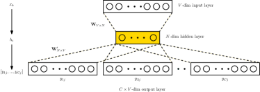
Figure 1. The Skipgram model uses two vector representations $\mathbf{W}$ and $\mathbf{W^{\prime}}$ to predict the context vertices from a single input vertex.

Given a network of users connected with unweighted edges, random walks are generated by repeatedly sampling an integer uniformly from {1,2,…, $D_{v}$} where $D_{v}$ is the vertex degree and moving to a new vertex. Concretely, for a random walk starting at vertex $v_{0}$ we would sample $x\sim U(\{1,2,\dots,D_{v_{0}}\})$ where U is a uniform distribution and $D_{v_{0}}$ is the degree of $v_{0}$. If $x=1$ we move to the lowest indexed neighbour of $v_{0}$, append that vertex to the random walk and repeat the process at vertex $v_{1}$.

2.2. The Skipgram Model on User Sequences

After we have sampled user sequences with random walks, we can use them to train user embeddings. There are several related embedding models, i.e. SkipGram and Continuous Bag of Words (Mikolov et al., 2013). Here we adopt the SkipGram with Negative Sampling (SGNS) model that is depicted in Figure 1. The figure shows a shallow neural network with a single hidden layer and two separate vector representations labelled as W and W’. The input to SGNS is a sequence of users, which are mapped to (input, context) pairs by sliding a context window over the input sequences. The input user representation is in W and the neighbouring (i.e. context) users share a representation in W’. Users are initially randomly allocated within the two vector spaces and then the model is trained using Stochastic Gradient Descent (SGD). The objective function gives the probability of the context users given the input user, which is modelled by a softmax. We optimise the negative log likelihood given by

(1) $$L =-\log p(w_{o,1},w_{o,2},w_{o,3},...,w_{o,C}|w_{I})$$

(2) $$=-\log\prod_{c=1}^{C}\frac{\exp{\mathbf{v}^{{}^{\prime}T}_{c}}\mathbf{v}_{I}}{\sum_{j=1}^{V}\exp{\mathbf{v}^{{}^{\prime}T}_{j}\mathbf{v}_{I}}}$$

where $w_{(.)}$ is a user and $\mathbf{v}_{(.)}$ and $\mathbf{v}_{(.)}^{{}^{\prime}}$ are the input and output vector representations of that user and $C$ is the context size, typically ten. In practice, it is expensive to evaluate Equation (2) as the sum in the denominator is over all of the users in the network. Instead we use negative sampling, which is a form of Noise Contrastive Estimation (NCE) (Gutmann and Hyvärinen, 2012), to estimate the function by only evaluating a small number of negative samples in addition to the observed positive example. The gradient descent update rules for a user pair $(w_{I},w_{O})$ with vector representations $(\mathbf{v}_{I},\mathbf{v}^{\prime}_{O})$ are found by applying the chain rule to Equation (2) and are given by

(3) $$\mathbf{v}_{j}^{{}^{\prime}new} =\begin{cases}\mathbf{v}_{j}^{{}^{\prime}old}-\eta(\sigma(\mathbf{v}_{j}^{{}^{\prime}T}\mathbf{v}_{I})-t_{j})\mathbf{v}_{i},&w_{j}\in\chi\\ \mathbf{v}_{j}^{{}^{\prime}old},&\text{otherwise}\end{cases}$$

where $\chi=\{w_{O}\}\cup W_{neg}$. For the output representation and

(4) $$\mathbf{v}_{I}^{new} =\mathbf{v}_{I}^{old}-\eta\sum_{j:w_{j}\in\chi}(\sigma(\mathbf{v}^{{}^{\prime}T}_{j}\mathbf{v}_{I})-t_{j})\mathbf{v}^{\prime}_{j}$$

for the input representation. In these equations $t_{j}$ is an indicator variable that is one if and only if $w_{j}=w_{O}$ and zero otherwise, $\eta$ is the SGD learning rate and $W_{\rm neg}$ is the set of negatively sampled users. We follow (Mikolov et al., 2013) and draw $W_{\rm neg}$ from the distribution of users in the random walks raised to the power of $\frac{3}{4}$.

3. Experimental Setup

C	Title	U
1	Managers, Directors and Senior Officials	461
2	Professional Occupations	1615
3	Associate Profess. and Technical Occupations	950
4	Administrative and Secretarial Occupations	168
5	Skilled Trades Occupations	782
6	Caring, Leisure and Other Service Occup.	270
7	Sales and Customer Service Occupations	56
8	Process, Plant and Machine Operatives	192
9	Elementary Occupations	131
Total		4625

Table 1. Distribution of users (U) across occupational classes (C).

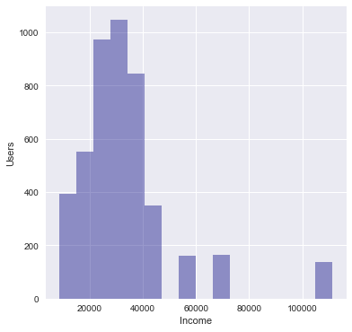
Figure 2. Distribution of users and income. Income is calculated in British pounds (£).

3.1. Data

We experiment using two publicly available datasets that contain Twitter users mapped to their occupational class and income (Preoţiuc-Pietro et al., 2015b, a). The datasets contain the same group of 5,191 users in total. However, some of the accounts are not considered in our experiments since we were not able to extract their social network information. These accounts may have been deleted or become private since the release of the datasets. Therefore, we report results on a subset of the original set of users, i.e. 4,625 users, that are still publicly available.

Occupational Class

Users are mapped with an occupation using the Standard Occupation Classification (SOC) taxonomy devised by the Office of National Statistics in the UK, based on skill requirements. The SOC taxonomy has a hierarchical structure with 9 major groups (e.g managers or elementary occupations). Users in the dataset have been mapped to one of these major groups. Table 1 shows the distribution of users across the nine occupational classes. The Pearson’s correlation between the original distribution of users and our subset distribution is $0.93$.

Income

The occupational class of users has further been used as a proxy to infer their income from the Annual Survey of Hours and Earnings. The income represents the mean yearly earnings for 2013 in British Pounds (GBP) for each occupational class. Figure 2 shows the distributions of users and income in the dataset. The mean user income in the original dataset is $32,509.74$, while the mean of the subset we use in our experiments is $32,727.92$.

3.2. Implementation of the Graph Embeddings

To construct graph embeddings we downloaded the Twitter IDs of everyone followed by the $4,625$ accounts. This produced a set of $3,925,702$ users in total. We considered only accounts followed by at least 10 users, which reduced the number of the unique accounts to $53,199$. To produce sequences of users we treat the edges of the Twitter graph as undirected and take 80 step random walks initiated at each vertex in this network.

The dimensionality of the embedding affects the performance in predictive tasks. We experimented with dimensionalities of $16,32,64$ and $128$ and chose the optimal value following a nested 10-fold cross-validation approach as in Preoţiuc-Pietro et al. (2015a, b). We found that the best performing embedding dimensionality is 32. The user embeddings and the code to generate them are available to download from https://github.com/melifluos/income-prediction.

3.3. Predictive Models

Occupational Class

Predicting the occupational class of a user is defined as a 9-way classification task. Given a user feature representation, our goal is to assign the most probable class label. For that purpose, we use the graph embeddings as features and a concatenation of the graph embeddings with the topics introduced in (Preoţiuc-Pietro et al., 2015a) to train Logistic Regression (LR) (Zou and Hastie, 2005), Support Vector Machines (SVM) (Joachims, 1998) and Gaussian Process Classifiers (GPC) (Williams and Rasmussen, 1996). All of the classifiers are trained following the one-vs-all approach.

Income

Inferring income is defined as a regression task. Given the user feature representation as input, we try to predict a real value representing the user’s income. The goal is to minimise the absolute error between the actual and inferred income. We also compare three popular models: (1) linear regression (LR), (2) Support Vector Regression (SVR) (Drucker et al., 1997), and (3) Gaussian Process Regression (GPR) (Williams and Rasmussen, 1996).

4. Results and Discussion

Tables 2 and 3 show the results obtained by the proposed models using the graph embeddings (Graph) and their combination (Graph+Topics) as feature representations for users. Note that models using Topics (i.e. word frequency of user’s tweets in a set of 200 precomputed word clusters) and Temporal Orientation as features are the baseline methods presented in Preoţiuc-Pietro et al. (2015a, b) and Hasanuzzaman et al. (2017). To compare against Preoţiuc-Pietro et al. (2015b, a), we retrain these models using the user accounts in the dataset that are publicly available (see Subsection 3.1).

Occupational Class
Method	Accuracy (%)
Majority Class	35.00
Preoţiuc-Pietro et al. (2015a)
LR-Topics	46.57
SVM-Topics	49.47
GP-Topics	49.64
Ours
LR-Graph	46.24
SVM-Graph	50.14
GP-Graph	50.44
LR-Graph+Topics	48.84
SVM-Graph+Topics	52.00†
GP-Graph+Topics	51.46†

Table 2. Accuracy of models in predicting user occupational class.$\dagger$ denotes statistical significant different (t-test, $p<0.01$) method to GP-Topics.

Our best performing model using graph based features (Graph) achieves an accuracy of $50.44\%$ in the occupational classification task. In income prediction, the MAE is $9,048$ and Pearson’s correlation is $0.63$. This implies that graph embeddings carry meaningful information about user’s socioeconomic attributes making them an effective user representation. The graph embedding features perform consistently better than the textual features (Topics) for the majority of the predictive models on both tasks except for the LR model. This confirms our first hypothesis that information from the network structure of a user is indicative of socioeconomic attributes. Figure 3 shows a 2-d t-SNE plot of the best performing user embedding, where we observe many distinct “communities” of low and high income users that appear together. This confirms our assumption about the homophilic nature of the Twitter network.

The combination of user embeddings and topics (Graph+Topics) outperforms either feature set used individually. More specifically, our GPC-Graph+Topics model significantly outperforms (t-test, $p<0.01$) the previous state-of-the-art method, GPC-Topics introduced in Preoţiuc-Pietro et al. (2015a) on occupational classification. Moreover, our SVR-Graph+Topics model significantly outperforms ($p<0.001$) the best baseline method, i.e. SVM+Topics. This confirms our second hypothesis that network structure and linguistic information are complementary.

The above findings shed light on the homophilic behaviour of users on Twitter. That might have further implications on user behaviour when selecting friends and forming social networks online. Our results suggest that a stronger bias might exist towards selecting friends with common socioeconomic backgrounds in contrast to common topics of interest and that needs to be explored further.

Non-linear models (i.e. SVM, SVR, GPC, GPR) achieve better results in inferring user socioeconomic attributes than linear (LR) models. While in the occupational classification task our best performing model is GPC, the best model in income inference is the SVR instead of GPR. This implies that model selection is important in these tasks.

An analysis of the errors in the occupational classification task shows that most misclassifications come from adjacent classes. For example, users in classes 1, 3 and 4 are mistakenly classified as class 2. This happens because adjacent classes contain related occupations. However, we notice less dispersion of errors caused by other classes misclassified as class 2 when we use graph embeddings and the combination of graph embeddings and topics. This might be explained by the homophily of users’ networks captured by graph embeddings.

Income
Method	MAE (£)	$\mathbf{\rho}$
Preoţiuc-Pietro et al. (2015b)
LR-Topics	10573	.50
SVR-Topics	9528	.59
GPR-Topics	9883	.60
Hasanuzzaman et al. (2017)
LR-Temporal Or.	10850	.45
GP-Temporal Or.	10235	.51
Ours
LR-Graph	10811	.50
SVM-Graph	9048‡	.62
GP-Graph	9532	.63
LR-Graph+Topics	10326	.54
SVM-Graph+Topics	9072‡	.64
GP-Graph+Topics	9488	.64

Table 3. Mean Absolute Error (MAE) and Pearson’s correlation coefficient ($\rho$) between actual and predicted income. ${\ddagger}$ denotes statistical significant different (t-test, $p<0.001$) method to SVM-Topics.

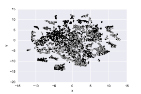
Figure 3. A 2-d t-SNE plot of the best performing user embedding (32D). Black and white represent users with above and below median income respectively.

5. Conclusions

We presented a method to reliably predict user occupational class and income on Twitter. Information from a user’s social network is represented by graph embeddings (Perozzi et al., 2014; Tang et al., 2015) and is used to train predictive models. To the best of our knowledge, this work is the first to introduce graph embeddings for automatically inferring socioeconomic characteristics. We also demonstrated that the information extracted from the user’s social network and their language use are complementary. That combination significantly improves predictive performance. Finally, our proposed models achieve state-of-the-art results in two standard datasets of income and occupational class, significantly outperforming previous methods.

References

- (1)
- Al Zamal et al. (2012) Faiyaz Al Zamal, Wendy Liu, and Derek Ruths. 2012. Homophily and Latent Attribute Inference: Inferring Latent Attributes of Twitter Users from Neighbors. In ICWSM.
- Bengio et al. (2003) Yoshua Bengio, Réjean Ducharme, Pascal Vincent, and Christian Jauvin. 2003. A Neural Probabilistic Language Model. JMLR 3 (2003), 1137–1155.
- Bernstein (1960) Basil Bernstein. 1960. Language and social class. The British Journal of Sociology 11, 3 (1960), 271–276.
- Bernstein (2003) Basil Bernstein. 2003. Class, codes and control: Applied studies towards a sociology of language. Vol. 2. Psychology Press.
- Burger et al. (2011) John D Burger, John Henderson, George Kim, and Guido Zarrella. 2011. Discriminating gender on Twitter. In EMNLP. 1301–1309.
- Campbell et al. (1986) Karen E Campbell, Peter V Marsden, and Jeanne S Hurlbert. 1986. Social resources and socioeconomic status. Social Networks 8, 1 (1986), 97–117.
- Chamberlain et al. (2017) Benjamin Chamberlain, Clive Humby, and Marc Peter Deisenroth. 2017. Probabilistic Inference of Twitter Users’ Age based on What They Follow. In ECML-PKDD. 191–203.
- Cheng et al. (2010) Zhiyuan Cheng, James Caverlee, and Kyumin Lee. 2010. You are where you tweet: a content-based approach to geo-locating Twitter users. In CIKM. 759–768.
- Cohen and Ruths (2013) Raviv Cohen and Derek Ruths. 2013. Classifying political orientation on Twitter: It’s not easy!. In ICWSM.
- Conte et al. (2012) Rosaria Conte, Nigel Gilbert, Giulia Bonelli, Claudio Cioffi-Revilla, Guillaume Deffuant, Janos Kertesz, Vittorio Loreto, Suzy Moat, Jean-Pierre Nadal, Anxo Sanchez, and others. 2012. Manifesto of computational social science. European Physical Journal-Special Topics 214 (2012), 325–346.
- Dredze et al. (2016) Mark Dredze, Miles Osborne, and Prabhanjan Kambadur. 2016. Geolocation for Twitter: Timing Matters. In NAACL-HLT. 1064–1069.
- Drucker et al. (1997) Harris Drucker, Christopher JC Burges, Linda Kaufman, Alex Smola, Vladimir Vapnik, and others. 1997. Support vector regression machines. In NIPS. 155–161.
- Grover and Leskovec (2016) Aditya Grover and Jure Leskovec. 2016. node2vec: Scalable feature learning for networks. In KDD. 855–864.
- Gupta et al. (2013) Pankaj Gupta, Ashish Goel, Jimmy Lin, Aneesh Sharma, Dong Wang, and Reza Zadeh. 2013. WTF: The Who to Follow Service at Twitter. In WWW. 505–514.
- Gutmann and Hyvärinen (2012) Michael U Gutmann and Aapo Hyvärinen. 2012. Noise-contrastive estimation of unnormalized statistical models, with applications to natural image statistics. JMLR 13 (2012), 307–361.
- Han et al. (2014) Bo Han, Paul Cook, and Timothy Baldwin. 2014. Text-based Twitter user geolocation prediction. Journal of Artificial Intelligence Research 49 (2014), 451–500.