Natural Language Statistical Features of LSTM-generated Texts
Abstract
Long Short-Term Memory (LSTM) networks have recently shown remarkable performance in several tasks dealing with natural language generation, such as image captioning or poetry composition. Yet, only few works have analyzed text generated by LSTMs in order to quantitatively evaluate to which extent such artificial texts resemble those generated by humans. We compared the statistical structure of LSTM-generated language to that of written natural language, and to those produced by Markov models of various orders. In particular, we characterized the statistical structure of language by assessing word-frequency statistics, long-range correlations, and entropy measures. Our main finding is that while both LSTM and Markov-generated texts can exhibit features similar to real ones in their word-frequency statistics and entropy measures, LSTM-texts are shown to reproduce long-range correlations at scales comparable to those found in natural language. Moreover, for LSTM networks a temperature-like parameter controlling the generation process shows an optimal value—for which the produced texts are closest to real language—consistent across the different statistical features investigated.
Index Terms:
Long Short-Term Memory Networks, Natural Language Generation, Long-Range Correlations, Entropy, Authorship Attribution.I Introduction
Building artificial systems capable of mimicking human creativity has long been one of the aims of Artificial Intelligence (AI) [1]. In this work, we focus on the problem of Natural Language Generation (NLG), which encompasses the capability of machines to synthesize text in a way that resembles spoken or written language typically employed by humans [2]. This research field has recently known a period of great excitement, mostly due to the huge development in the area of deep learning [3], whose methods and algorithms have certainly contributed to move significant steps forward.
Deep learning techniques have in fact produced stunning results in a variety of different research fields and application domains, and one of the major successes has been that of generative models [4]. In the area of NLG, many studies have been dedicated to specific, focused applications, such as image and video captioning [5, 6], poem synthesis [7] or lyric generation [8]. In all these cases, the considered generated texts are relatively short (captions, poems, lyrics) and correlations between words rarely span across several sentences. The scenario totally changes when we consider longer texts, such as novels. Natural language has been widely studied within this context, and notoriously it shows statistical properties in the distribution of terms, as well as long-range correlations between words [9, 10, 11]. In comparison to short texts such as captions, this is a much more challenging setting to imitate for machines.
In this work, we aim to provide an extensive empirical evaluation of texts generated with Long-Short Term Memory (LSTM) networks, one of the most widely used deep learning models for NLG. Our goal is to quantitatively assess whether LSTM texts do share some similarities with natural language that is commonly produced by humans. To this aim, we trained an LSTM network with a corpus that consists of a collection of novels by Charles Dickens. Such network is trained to predict the next character of a given text, and thus it can be employed to iteratively generate a document of any desired length. The setting was adopted in several works (e.g., see [12, 13] and citations therein).
In our experimental framework we evaluated several different aspects of machine-generated texts, comparing them against the statistics of real language and Markov-generated samples. First, we analyzed fundamental linguistic properties typically shown by texts, such as Zipf’s [14] and Heaps’ [15] laws for words. Second, we studied whether the generated texts presented long-range correlations, which are commonly encountered in human-generated texts, but difficult to reproduce for machines. As a third point, we compared the entropy of the generated texts with the one of the original corpus. We then moved our analysis to a higher level, by carrying out a preliminary study looking at characteristics dealing with the style and quality of the generated texts: in particular, we analyzed the degree of creativity and plagiarism of the artificial texts with respect to the dataset on which the LSTM was trained, by looking at longest common subsequences. We also assessed whether an authorship attribution algorithm would capture some analogy between the generated text and the original one, in terms of author’s style.
Surprisingly, very few studies have been dedicated to a thorough analysis and to a quantitative evaluation of the similarities between texts created by machines and texts created by humans. Karpathy et al. [13] also provide an experimental analysis of LSTM networks trained for character-by-character text generation, but they focused their study on a qualitative evaluation of the cell activations within the neural architecture: for example, they looked for open and closed parentheses or quotes, that typically span a few tens or hundreds of characters. Their claim that the LSTM model is capable of capturing long-range dependencies is thus only supported by such qualitative evidence, without giving a deep insight in the characteristics of the generated documents. Lin and Tegmark [16] compared natural language texts with those generated by Markov models and LSTMs, exploiting metrics coming from information theory. Their analysis shows that LSTMs are capable of capturing correlations that Markov models instead fail to represent, yet the range of correlations they consider is still quite limited (up to 1,000 characters). Conversely, Takahashi and Tanaka-Ishii [17] reported that LSTM language models have limitation in reproducing such long-range correlations if measured with a method based on clustering properties of rare words; note however that their analysis is still limited to a range of 1,000 words, and the corpus they employ for training is much smaller than the one used in our experiments. Ghodsi and DeNero [18] instead, analyzed some statistical properties of text generated by a Recurrent Neural Network Language Model (RNNLM), in particular focusing on the length of sentences, the vocabulary distribution, and the distribution of specific grammatical elements, such as pronouns. In a complementary study, Lake and Baroni [19] focused on short-scale structures instead of the overall statistical properties of pseudo-texts. They showed that RNNs are able to exploit systematic compositionality, and thus also to reproduce, for example, abstract grammatical generalizations.
The remainder of the paper is organized as follows. Section II will describe the LSTM model used in our experiments. Section III will present the statistical methods employed for the quantitative evaluation of the artificial text properties. Section IV will describe the corpora used to train our model, and Section V will report and discuss the experimental results. Section VI will finally conclude the paper, also pointing for future research directions.
II Long Short-Term Memory Networks
Long Short-Term Memory networks (LSTMs) are recurrent neural networks (RNNs) that have been first developed at the end of the 90s, achieving remarkable results in applications dealing with input sequences [20]. Such model was specifically designed to address the issue of vanishing gradients, that greatly limited the applicability of standard RNNs [21]. Within the “deep learning revolution” that Artificial Intelligence has been undergoing in the last decade, LSTMs have regained popularity, being now widely used in a huge number of research and industrial applications, including automatic machine translation, speech recognition, text-to-speech generation (e.g., see [22] and references therein).
II-A General framework
RNNs allow to process sequences of arbitrary lengths, by exploiting hidden layers , with whose cells are functions not only of the layer input , but also of the hidden layer at the previous time step: . RNNs are typically trained with Backpropagation Through Time (BPTT) [23], by unfolding the recurrent structure into a sort of temporal chain through which the gradient is propagated, up to a certain number of time steps. Unfortunately, this method suffers from the well-known problem of vanishing or exploding gradients [20, 21], which makes plain RNNs scarcely used in practice. LSTMs overcome this issue by exploiting a more complex hidden cell, namely a memory cell, and non-linear gating units, that control the information flows into and out of the cell.
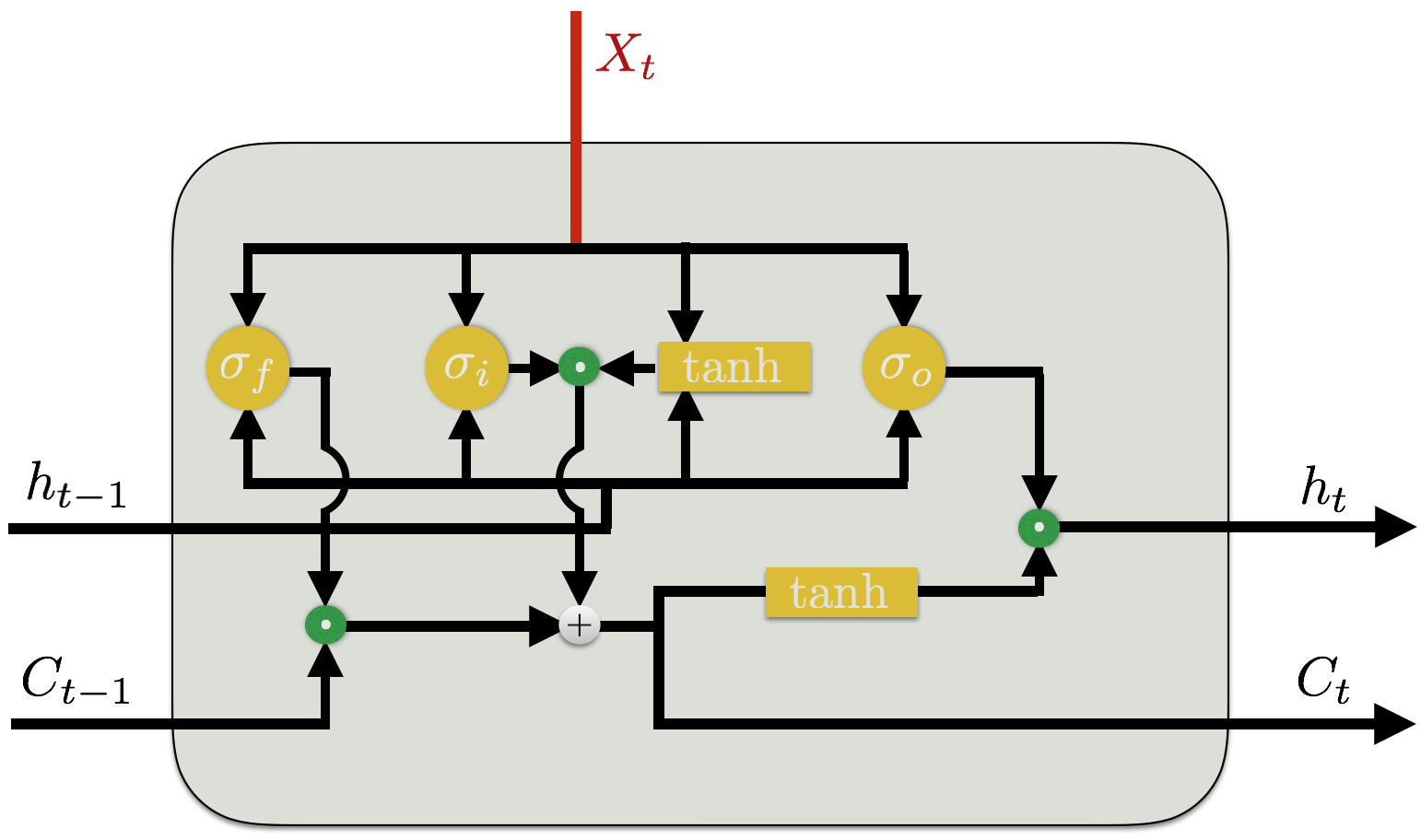
Basically, the LSTM cells are capable of maintaining their state over time, of forgetting what they have learned, and also of allowing novel information in. An example of such a cell is depicted in Figure 1. The model is based on the concept of cell status at time , namely , which depends on three gates: an input gate that can let new information into the cell state, a forget gate that can modulate how much information is forgotten from the previous state, and an output gate that controls how much information is transferred to the upper layers. The following equations describe the behaviour of an LSTM layer (we drop the layer index in order to simplify the notation):
| (1) | ||||
| (2) | ||||
| (3) | ||||
| (4) | ||||
| (5) |
where all are typically the sigmoid function, indicates the Hadamard (or element-wise) product, and , , represent the model parameters that have to be learned. As a form of regularization, dropout is nowadays typically employed in deep neural networks [24]. Dropout simply consists in randomly dropping a percentage of connections between neurons during training, while multiplying by every weight in the network at testing time. In recurrent architectures, though, this general framework does not work well in practice, but dropout can still be successfully employed, if applied only to inter-layer connections and not to recurrent ones [25]. This is how we employed dropout in our model.
II-B LSTM for text generation
The most widely employed LSTM architecture for text generation is based on character-level sentence modeling. Basically, the input of the network consists in characters, that correspond to a fixed-size portion of text, whereas the number of output neurons is the total number of possible symbols in the text, each neuron corresponding to one of such characters. The output layer consists in a softmax layer, so that each symbol has an associated probability, and all such probabilities sum up to 1. A hard way of generating texts is to pick the character with the highest probability as the next one in the sequence, and to feed it back into the network input. A soft alternative (which is the one used in practice) allows to sample the next character in the sequence from the probability distribution of the output cells: in this way the output of the network is not deterministic, given the same initial input sequence. With such an iterated procedure, texts of any length can be generated. The hidden states of the cells keep track of the “memory” of the network, so as to exploit also information not directly encoded in the input any more. This generation phase can be controlled by a parameter , usually named temperature. Different temperature values can be tuned in order to obtain a smoother or sharper softmax distribution from which characters are generated: in particular, the final softmax layer in the LSTM computes the probability of each symbol as follows:
| (6) |
where are the output values for each symbol that are fed into softmax. Large values lead towards a uniform distribution of symbol probabilities, whereas when tends to zero, the distribution is skewed towards the most probable symbol.
Such a model is trained in a classic supervised learning setting, where the input training corpus is fed to the network, using as target the true (known) next character, as it appears in the corpus. If the cell states are not reset as subsequent input windows are presented to the network, long-range dependencies can in principle be captured by the model.
Note that, in principle, the same task could be modeled at a word level, thus training the LSTM network to predict the next word in the text, rather than the next character. Although this solution may appear a more appropriate way for modeling the problem, it has two main limitations: (i) the number of possible output classes of the network would become huge, being the total number of distinct words in the input corpus, leading to a much more difficult optimization problem, which would likely require a larger number of training examples; (ii) the set of possible output words would be limited to those appearing in the training corpus, which could be enough in many cases, but would limit the creativity of the network.
III Methods
We now present the methods we employ in order to quantitatively evaluate the characteristics of the artificially generated texts with respect to the original, human-generated texts.
III-A Zipf’s and Heaps’ laws for words
Natural languages show remarkable statistical properties in their word statistics. The two best known examples are Zipf’s [14] and Heaps’ [15] laws in language, which refer to universal features related to word frequencies.
Zipf’s law states that if the word frequencies of any sufficiently long text are arranged in decreasing order, there is a power-law relationship between the frequency and the corresponding ranking order of each word. More explicitly, if we denote the rank of a word by , the Zipf’s law states the following relationship between the rank and the frequency of a word at that rank position , as follows:
| (7) |
This relationship is roughly the same for all human languages, the exponent taking values close to 1.
Heaps’ law states that the number of the different words (i.e the size of the vocabulary) after seeing consecutive words in a text, obeys approximately the following relationship:
| (8) |
with exponent typically taking values smaller than 1 [26].
III-B Long-Range Correlations
Linguistic laws on the scaling of word frequencies, like Zipf’s and Heaps’, do not reveal any statistical structure that depends directly on word order. Zipf’s rank-frequency distribution would be unaltered after a random text shuffling, and similarly for the average behaviour predicted by Heaps’ law. Statistical measures that capture structure at the sequence level in texts involve correlations and spectral analysis [27].
Correlations in language are known to be of the power-law type [9, 10, 11], decaying as , where is the distance between symbols – e.g. words or characters. It is possible to characterize the structure of long-range correlations using the method of Detrended Fluctuation Analysis (DFA) [28, 29]. The first step in the method involves the mapping of the symbol sequence onto a numerical time-series, by assigning a number to each basic symbol in the sequence. In order to preserve the maximum of structure from the text sources, we performed the mapping at character level—including all punctuation signs, numbers, capital letters, and accented forms. The procedure to assign a number to each character followed similar lines to the method employed in [10], where in the present case each character is replaced by its rank. Thus, the most frequent character is assigned the number 1, the second most frequent the number 2, and so on. For a sequence of length , the character at position in the time series, with , can be represented by the number , and the following random-walk can be constructed:
| (9) |
where represents the mean of the times series. The time series is then split into windows of length , and in each of those windows the corresponding stretch of the series is fitted by a straight line by means of least squares. These linear fits represent the local trend within each of the windows of length . The sequence of length- trends can be concatenated in a piecewise manner defining a piecewise linear function . Then we compute the average fluctuations at scale , that is the deviations from the trend, defined as follows:
| (10) |
The nature of the correlations present in the original time series can be evaluated by observing the dependence of on . In particular, the growth of fluctuation with the scale will be given as , with . In the case of an uncorrelated or short-range correlated time series , we have . However, in the presence of long-range correlations of the power-law type in the original time series , the fluctuation exponent will differ from [29], with for persistent (positive) correlations and for anti-persistent (negative) correlations.
III-C Entropy and KL-divergence estimation
The entropy of a symbolic sequence can be interpreted as a quantification of the degree of predictability in the sequence. A high level of predictability of consecutive values in a sequence implies a low level of surprise about future symbols, which is linked to a low entropy. On the other hand, a sequence with a high degree of randomness will be characterized by a high level of surprise in the identity of future symbols, and result in a high value for the entropy. Therefore, the determination of the entropy of language serves as a quantification of its degree of order. Early attempts to determine the entropy of language were based on the close link between entropy and predictability [30]. However, the estimation of the entropy from long sequences of written text, requires the estimation of block probabilities, which poses a serious computational challenge, due to the presence of long-range correlations in language. The required sample size needed for an accurate estimation of the block probabilities grows exponentially with the length of the block, thus quickly rendering insufficient any available amount of text. This difficulty can be overcome through the link between entropy and predictability mentioned above. The degree of predictability in a sequence determines how much it can be compressed by a lossless compression method. Sequences with high predictability can be compressed more than sequences with a higher degree of randomness. In particular, it can be shown that under general assumptions of stationarity and ergodicity, the entropy rate of a stochastic source is a lower bound to the length per symbol of any encoding of it [31]. Hence, the entropy of symbolic sequences can be estimated by means of efficient lossless compression algorithms [32, 33, 34]. We estimated the entropy of long character sequences using an implementation of the algorithm proposed by Lempel and Ziv [32, 35, 36], which relies on the estimation of redundancy by looking for matches between future and past substrings in a symbolic sequence. Implementations of entropy estimation algorithms based on these methods have proved to work well for symbolic sequences even in the presence of long range correlations as those found in language [34, 37].
The Kullback-Leibler (KL) divergence is a measure of relative entropy between two probability distributions and [31]. When then the KL-divergence is zero, but it takes positive values when . It can be shown that the is a measure of the extra numbers of bits that are required to encode typical sequences with the distribution , when using a code based on [31]. This interpretation suggests that can also be estimated using compression algorithms in which one signal is compressed using past sequences in the second signal. More specifically, the KL divergence can be written as [31]
| (11) |
where is the entropy of the distribution and is the cross-entropy between and . Let us assume that two text sequences produced by the stochastic source with probability distribution are represented by , and those produced by as . Then, for notational succinctness let us write the information quantities explicitly in terms of the generated sequences, therefore representing the KL-divergence between and as . With this notation, we have . A compression-based algorithm proposed in [38] permits to compute the cross-entropy based on the symbolic sequences and . Then, the KL-divergence is obtained by subtracting the entropy of the sequence from the cross-entropy . The KL divergence is a non-symmetric quantity and in order to have a distance-like measure between character sequences and , we defined a symmetrized divergence as .
Another measure that is strictly related to entropy, and that is widely used for the evaluation of artificial texts, is perplexity [39], which can be computed as the geometric mean of the inverse probability for each predicted word in the a document [40, 41], where probabilities are typically estimated on a language model trained on a larger corpus.
III-D Creativity and Authorship Attribution
Providing a quantitative method able to address the creativity of a given algorithm for artificial texts generation is a complex task. In this paper we consider two distinct yet strictly intertwined aspects: we aim to measure at what extent the algorithm is capable of capturing the stylistic traits of a given author, while, at the same time, avoiding to perform just a plagiarism of the training corpus.
Measuring the Longest Common Subsequence (LCS) is one of the simplest way to implement the idea of quantitatively measuring plagiarism: given the -th character of the artificial text, we denote by the length of the longest subsequence starting at that is also contained in (thus, plagiarized from) the training corpus. Different statistics of the set of all can be used to quantify how various algorithms are able to reproduce some stylist traits of a given corpus while generating innovative texts, not written before. Here we adopt the simplest one and consider the maximum over the whole artificial text: (see [42] and [43]).
We now move our analysis to a higher level, by exploring how artificial texts resemble the style of the training author. Stylistic traits are supposed to reflect subtle choices of the author in terms of vocabulary, syntactic constructions and structural composition, to mention a few. As such, a comprehensive quantification of the style of an author is out of reach. On the other hand, a very simple feature such as the frequency distribution of -gram of letters has been successfully selected as a key ingredient in some of the most effective approaches to authorship attribution [44, 45].
We use one of the state-of-the-art algorithms to test the automatic attribution of the author of our artificial texts. The implemented method is in fact one of the two methods that have been succesfully used for the attribution of Antonio Gramsci’s papers [44]. Essentially, each method defines a kind of similarity distance between texts. Let us very briefly describe just the first method used here, referring to [45] for further details. The method is based on (characters) -grams and it is probably one of the simplest possible measures on a text: after a first experiment based on bigram frequencies presented in 1976 by Bennett [46], Kes̆elj et al [47] published in 2003 a paper in which -gram frequencies were used to define a similarity distance between texts (see also [48]). The similarity distance was introduced and discussed in [44]: we call an arbitrary -gram, and we denote by and the relative frequencies with which occurs in text and . is the -gram dictionary of text , that is, the set of all -grams which have non-zero frequency in (similarly for ) and we define what we will call the -gram distance between text and text as111To be more precise, is a pseudo-distance, since it does not satisfy the triangle inequality and it is not even positive definite: two texts can be at distance without being the same.:
| (12) |
where the denominator is the sum of the number of different -grams in the two dictionaries, respectively, while the inner sum is taken over all the different -grams occurring in the two texts.
Suppose the goal is to decide whether a given document has been authored by author or not. The approach adopted in [44] consists in first collecting documents from author and documents from an author (or, in general, from more authors). The distance of the candidate text to these documents is then used, with the help of a simple probabilistic method, to produce a similarity index , (see [44] for details on the method). Values of the index close to (respectively, ) reveal a very strong attribution to author (respectively, ), while values close to 0 indicate a very weak attribution (see [44, 45] for more details).
IV Corpora
Our aim was to train an LSTM network on a large corpus obtained from a single author, in order to perform also the experiments on authorship attribution and to assess whether the model was capable of capturing some stylistic features of its “teacher”. We employed the works by Charles Dickens, since he was a very prolific author whose bibliography is freely available in plain text format at ProjectGutenberg.222http://gutenberg.org We collected a total of eighteen works by Charles Dickens, which resulted in a corpus of over 24 millions characters.333We used the following works: A tale of two cities, David Copperfield, Oliver Twist, Bleak house, Great expectations, The life and adventures of Nicholas Nickleby, The old curiosity shop, The Pickwick papers, Dombey and son, Little Dorrit, Life and adventures of Martin Chuzzlewit, Our mutual friend, Barnaby Rudge, A Christmas carol, The uncommercial traveller, Hard times, Letters, A child’s history of England.
For the authorship attribution experiments, we also collected a smaller corpus of texts, some still from Charles Dickens, and some others from a different author. Clearly, these additional texts from Dickens needed to be disjoint from those in the larger corpus, on which the LSTM network had to be trained.444We used excerpts from the following works: Signal-man, A Christmas tree, The poor relation’s story, The schoolboy’s story, Hunted down, Pictures from Italy, The chimes, The haunted man and the ghost’s bargain, Tom Tiddler’s ground, The wreck of the Golden Mary. Regarding non-Dickens documents, we collected texts by Robert Louis Stevenson, who was also a prolific author of the XIX century.555We used excerpts from the following works: Treasure island, The strange case of Doctor Jekyll and Mister Hyde, Kidnapped, The Black Arrow. For this second corpus, we collected 30 documents both for Dickens and for Stevenson, each consisting of 10,000 characters.
V Experiments
The experiments with LSTMs were run using the torch-rnn package.666https://github.com/jcjohnson/torch-rnn We trained an LSTM network with two layers and 1,024 cells in each layer. As customary in text generation experiments with LSTMs [13], the training set was split into chunks of length equal to characters: in this way, gradients in truncated backpropagation are propagated up to steps back, but the status of each LSTM cell is not reset after each example, so that longer-range correlations can in principle be learnt. We firstly present results obtained using , later investigating the impact of such hyper-parameter on the considered evaluation metrics. To avoid overfitting, a dropout equal to 0.7 was applied, and a validation set (4% of the whole corpus) was exploited to monitor the loss function during training.
To compare the statistics of the LSTM texts with that of other non-trivial models, we used a plain -order Markov process as a baseline. A family of -order Markov models were trained from our corpus, with taking values 2, 4, 6, 8, 10, and 12. The models were used to generate artificial texts starting from a seed taken from the original corpus.
Tables I and II show some examples of texts generated with different temperatures from the LSTM, and by different Markov models, respectively. The whole set of generated samples is publicly available at http://agentgroup.unimore.it/Lippi/generated_samples_Dickens.zip.
| LSTM generated text | |
|---|---|
| 0.1 | I had no doubt that I had no doubt I had no sooner said that I had no sooner said |
| that I had no sooner said that I was a stranger to me to see him | |
| 0.3 | I will not see him as I have been the family of my heart and expense, |
| and I should have seen him so soon. | |
| 0.5 | ’I am sure I think it is,’ said the doctor, looking at him at his heart on the window, |
| and set him there for a short time, ’that I shall find the girl there. | |
| 0.6 | The old man entered the other side, and then ascended the key on his shoulder. |
| ’I think I have no doubt, sir,’ replied the woman. | |
| 0.7 | ’I can refer to the world,’ said Mr. Tupman, suspiciously, |
| ’that the same brother was on the provoked passage.’ | |
| 0.8 | You look at me, you know I don’t think it should be what I have understood. |
| I know what she has of no confidence, and I have first cheered you. | |
| 0.9 | And so the position and paper escaped you by the Major, with the neck, |
| by my own evening, that there was a shadow of it. | |
| 1.0 | This interference of point that was always large in the evening, which was, |
| and used to save the crooked way, and could leave the undertakers upon it. | |
| 1.2 | Softly. They rose and who faithfully as stalled off, and his distrust |
| in the tip of which power it was. | |
| 1.5 | As if us, she Immoodnished Mrs Jipe Town horsemaking, |
| like the nights foldans with mid-yoUge false. Half-up? | |
| 2.0 | Connursing, visibly; brassbling, on what cohn; or’Pertixwerkliss issuin’p). |
| haf-pihy; and he-carse masls anycori’; nod me: full, nor cur your two yellmoteg’ | |
| 3.0 | ’Siceday; Quaky o’k, ,-GNIRRZVRIIMoklheHw, eab-mo,’_ ventvedes.r.’ |
| Egg_iglazzro!’wM’. ’Sav nam. Ebb-_Edjaevi.” |
| order | Markov generated text |
|---|---|
| 2 | ’And Mr Butentime ther foreweemair Masperf torto lit, ’It make to to yesee!” |
| shis thed to goin blie, thave com of a dess at’s mand havestroult frot own: ady. Saint | |
| 4 | But the Nation, and you in looking at all,’ said Mrs. Kenwigs’s hospite as I have gover with now, |
| ’and the eyes. Perhaps, and even to help, ‘I am sure loving her, | |
| 6 | Sam eyed Oliver, with some to her motion of the ladies, which at no immense |
| mob gathering which the after all the adorned to nod it, Sir!’ said Fledgeby | |
| 8 | The foot of the medical manner, ”Jenny saw, asserting to the large majority, |
| just outside as he had hardly achieved to be induced the room. | |
| 10 | I endeavour to get so precious contents, handed downstairs with pleasure the great Constitutions. |
| It happened to him like a man, and the fallacy of human being accepted lover of the tide | |
| 12 | Mr Witherden the notary, too, regarded him; with what seemed to bear reference to the friar, |
| taking this, as it served to divert his attention was diverted by any artifice. |
A)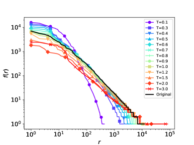 B)
B)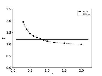
C)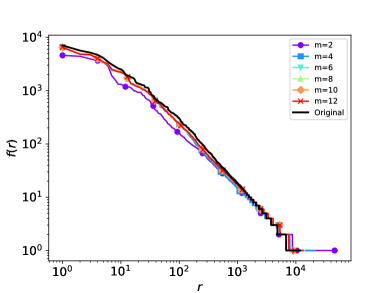 D)
D)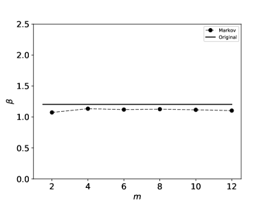
A)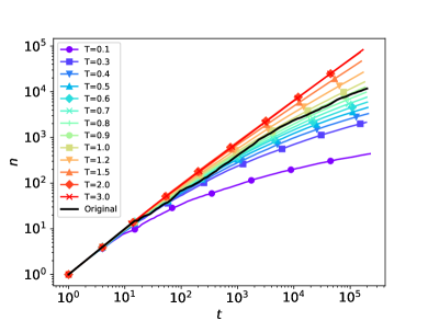 B)
B)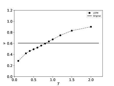
C)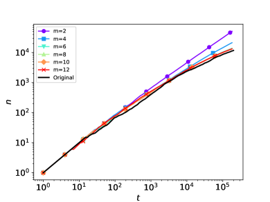 D)
D)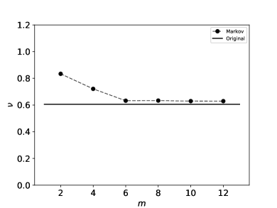
V-A Zipf’s and Heaps’ Laws
As a first test comparing the statistics of the LSTM-generated texts to other models capable of rendering stochastic versions of texts, we looked and the distribution of words frequencies. We first evaluated the Zipf’s law, by measuring the relationship between the rank in the set of words, ordered by frequency, and word frequency itself. Figure 2A shows the rank-frequency distributions of words in the LSTM texts for temperatures in the range 0.1-3.0. The plot also shows in black the result for the original Dickens corpus. We fitted the value of the exponent within the region between ranks and to determine more clearly the behavior with temperature, which showed a clear power-law behaviour consistently across all but the two extreme temperatures. Figure 2B shows the resulting value of the Zipf’s exponent as a function of temperature in the range 0.3-2.0. LSTM texts generated with low temperatures have a frequency rank distribution which decays faster with rank. On the contrary, for higher temperatures the distribution flattens, showing a smaller exponent . The dashed line in the figure shows the value of the exponent estimated from the Dickens’ corpus, which intercepts the LSTM results at a temperature between 0.8 and 0.9, approximately.
A similar analysis was performed on the Markov-generated texts. Figure 2C shows the rank-frequency distribution for texts generated with Markov models. Interestingly, there is little variation of the distribution as a function of Markov order. This is also corroborated by the estimation of the exponent (Figure 2D), which shows the exponent of Markov texts with a value slightly below that of the original source.
In order to assess the validity of Heaps’ law for the artificial language, we computed the statistics of the vocabulary growth for the LSTM and Markov texts. Figure 3A shows the results for the LSTM texts for a range of temperatures from 0.1 to 3.0. For comparison, the curve for the original text is shown in black. Figure 2B represents the results of fitting the power-law behavior in the region for , using the same range of temperatures shown for the exponent in Figure 2B. The dashed line, which represents results for the original text, cuts the LSTM data at a point between temperatures 0.8 and 0.9.
A)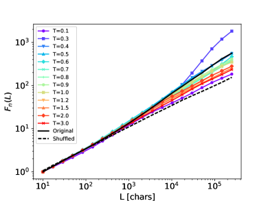 B)
B)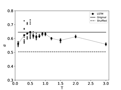
C)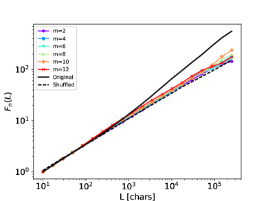 D)
D)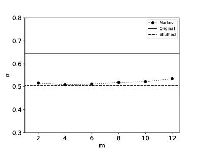
A)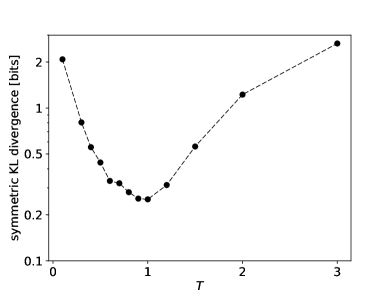 B)
B)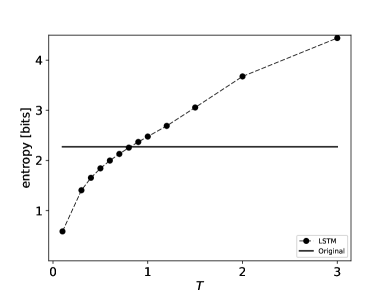
C)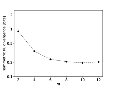 D)
D)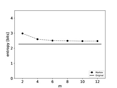
V-B Long-Range Correlations
Beyond the statistics of word frequencies, natural texts show correlations that span hundreds or thousands of characters, showing power-law decay. While a direct measure of these correlations is possible in principle, more efficient methods are based on spectral [27] or fluctuation [28, 29] properties of the sequences. In particular, we tested the LSTM generated texts using Detrended Fluctuation Analysis (DFA) [28, 29] applied to linguistic character sequences. By means of DFA it is possible to estimate such exponent , by fitting a power law to the the dependence of the fluctuations with the scale . We estimated the dependence of with the scale for LSTM texts generated at different temperatures and for the Markov-generated texts for different orders. Figure 4A shows the normalised fluctuations as a function of the scale for LSTM-generated texts together with the results for the original Dickens’ corpus and a shuffled realisation of it. In all cases there are signs of power-law behavior for a wide range of scales, with the exception of the two extreme temperatures (0.1 and 3.0). Although the data corresponding to the shuffled text seems to have a less steep slope than the LSTM samples, a more quantitative analysis is required to compare the extent of correlations. Figure 4B shows the estimations of the exponent obtained by fitting a power-law to the data in panel A in the region spanned by scales . For comparison, the full black line corresponds to the result for the original Dickens’ text while the dashed line is the result obtained from the shuffled text. The full black circles are the average of the estimation of the exponent from the 10 available samples, whereas small squares show the result for each sample. It is in the region between of temperatures between 0.5 and 1.0 that the exponent es closet to the value for the original text. Yet, while the dispersion of individual sample measures are very broadly spread for temperatures close to 0.5 they are tightly clustered around the mean for . A similar analysis was done on the Markov-generated texts. Figure 4C shows the result of the DFA for Markov texts of orders 2–12, and a comparison to the original and shuffled texts: clearly, all the Markov-generated texts have a structural correlation that resembles more the shuffled text than the original one. This trend is corroborated in Figure 4D, showing the estimated exponent as a function of Markov order. In all cases, such value is very close to that obtained by the shuffled text.
V-C Entropy
Our final test to probe the statistical structure of the LSTM texts consisted in the estimation of entropy measures. The first estimation corresponded to a symmetrized KL-divergence (see Section III) between the LSTM for different temperatures and original text, estimated by means of compression algorithms that are sensitive to the long-range structure of the signal. Figure 5A shows the divergence as a function of . There is a well-defined minimum at , indicating that at that temperature the structure of the LSTM text is closest to the original. Figure 5C shows a similar plot for Markov texts, which also approximate the structure of the original texts asymptotically for larger orders. While the previous analyses showed the behavior of a distance-like quantity, the entropy is a more direct estimation of the statistical structure of a signal. Panels B and D in Figure 5 show the value of the entropy for the LSTM and Markov texts as a function of the temperature and order respectively. In both cases the solid line corresponds to the value of the entropy of the original text. For LSTM, lower values produce texts with small entropy, thus easier to compress, since they show repetitive patterns. As grows, entropy also grows, with the texts becoming the most similar to the original around (in line with our analyses) and far more disordered for larger values. Markov texts, instead, show a monotonic approximation to the entropy of the original text, slightly above even for higher orders.
To complete the analysis, we also computed the perplexity of LSTM-generated texts, using the KenLM library777https://github.com/kpu/kenlm. To do this, we learned a bigram language model on the original Dickens corpus and then we computed the perplexity both for the artificial texts, and for the off-sample Dickens documents in the test corpus used for authorship attribution. Results are perfectly in line with those obtained with entropy computation via compression, with values of temperature around 0.9-1.0 producing texts that are the most similar to the original.
A)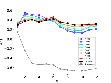 B)
B)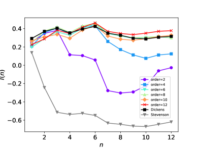
V-D Creativity and Authorship Attribution
To assess the degree of plagiarism (and, thus, of creativity) of our models, we measured the length of the Longest Common Subsequence (LCS) between the artificial texts and the training corpus. As for Markov texts, not surprisingly the length of the LCS rapidly grows with the order of the model, from a value of 19 for order 2, up to 73 and 125 for order 10 and 12, respectively. For LSTMs, the length of the LCS instead results to be lower, with values comprised between 40 and 60 when is in the range between 0.4 and 1.2. For smaller and larger temperatures, the LCS is clearly shorter, as the generated texts have a less realistic structure, thus it is less probable to encounter patterns identical to the original. As a comparison with what we could call a sort of self-plagiarism, encountered in a subset of the training corpus, we also computed the length of the LCS of the novel “Oliver Twist” with respect to five other novels by Dickens (David Copperfield, A Tale of Two Cities, Bleak House, Great Expectations, Hard Times): the LCS in this case resulted to be 45 characters long.
For the experiments on authorship attribution, we used the Dickens and Stevenson corpora described in Section IV. For a fixed temperature of the generated text, attribution is performed by averaging over samples of artificial texts, using -grams from up to . To assess the validity of the attribution algorithm, we compare the attribution of the generated texts with that of real texts. In particular, for each of the 30 Dickens and Stevenson documents, we employ the remaining 29 documents of each group to perform attribution to either author. Figure 6 shows the value of the index defined in Section III-D as a function of -grams (on the x-axis) and either temperature for LSTM (panel A) or order for Markov texts (panel B), respectively. The attribution of real texts performs extremely well, with a maximum for and for Dickens and Stevenson, respectively. For LSTM, while the texts are indeed always correctly attributed to Dickens, it is interesting to notice how the best results are again achieved for values of around 0.8-1.0, while for lower temperatures the attribution with larger -grams drops, as the generated texts tend to reproduce periodic (hence, less realistic) patterns. Not surprisingly, Markov texts with are also well attributed to Dickens, due to the high degree of plagiarism described in Section V-D.
V-E Impact of hyper-parameter
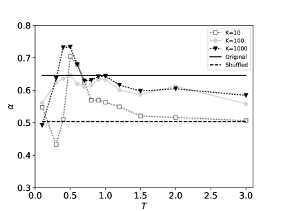
The results presented so far consistently show that there is a narrow range of temperatures around for which the texts generated by LSTM are the most similar to the original, in terms of all the considered metrics. We finally investigated the impact of hyper-parameter on the generated texts. Given that is the number of backward gradient propagation steps in the BPTT algorithm, it directly affects the way in which long-range information is propagated through the cells. Therefore, we considered two additional LSTM networks, trained with and , respectively, and identical to the first network for all the other settings. For all the considered metrics apart from long-range correlations, results are not significantly different from those obtained for the network trained with (see supplementary material for details). Long-range correlations are instead more significantly affected by the variation in . From Figure 7 we observe two different phenomena: (i) a peak for low-level temperatures, likely due to spurious, periodic patterns, that is visible also for (also notice the large variance across samples shown in Figure 4); (ii) a dramatic drop in the exponent for starting from , whereas for the exponent is much closer to that of real text.
VI Conclusions
In this paper, we investigated at what degree texts generated by an LSTM network resemble texts generated by humans. To this aim, we presented an extensive experimental evaluation where we compared several characteristics of artificial and original texts, starting from statistical properties typically shown by natural language, such as the distribution of word frequencies and long-range correlations, up to higher-level analyses, such as the attribution of authorship. Our study shows that LSTM-generated texts share key statistical features with natural language. In particular, the experimental results highlight the crucial role of the temperature parameter in producing texts that resemble those created by humans in their statistical structure, with an optimal range of temperatures, around , that induce the highest degree of similarity. Interestingly, we also illustrated how a network trained on a single-author corpus can produce texts that are attributed to that author, according to authorship attribution algorithms.
The presented study suggests many interesting research directions, which we plan to investigate in future works.
First, we aim to compare the semantic information of original and artificial texts. It is clear from the samples shown in the experimental section, that LSTM texts are still far from human-generated texts in terms of meaningfulness, although showing similar statistical properties. It is thus possible that certain correlates of semantic information, like burstiness and clustering of keywords, are reflected in LSTM texts. Given that even the origin of long-range correlations in natural language is still debated, our work paves the way to deeper future investigations in this direction.
Secondly, we aim to extend the analysis of these statistical properties of the LSTM texts to different languages, in order to assess whether there are some languages that are easier or more difficult to reproduce for a machine.
Finally, we aim to extend the study on authorship attribution and plagiarism, for which in this paper we only presented preliminary results. For that purpose we plan to employ a larger corpus, in order to compare several authors, genres and languages, and to test different algorithms, as for instance those based on trainable machine learning systems [49, 50].
References
- [1] M. A. Boden, “Creativity and Artificial Intelligence,” Artif. Intell., vol. 103, no. 1-2, pp. 347–356, 1998.
- [2] E. Reiter, R. Dale, and Z. Feng, Building natural language generation systems. MIT Press, 2000, vol. 33.
- [3] Y. LeCun, Y. Bengio, and G. Hinton, “Deep learning,” Nature, vol. 521, no. 7553, pp. 436–444, 2015.
- [4] Y. Bengio et al., “Learning deep architectures for AI,” Foundations and trends® in Machine Learning, vol. 2, no. 1, pp. 1–127, 2009.
- [5] A. Karpathy and L. Fei-Fei, “Deep visual-semantic alignments for generating image descriptions,” in Proceedings of the IEEE Conference on Computer Vision and Pattern Recognition, 2015, pp. 3128–3137.
- [6] S. Venugopalan, M. Rohrbach, J. Donahue, R. Mooney, T. Darrell, and K. Saenko, “Sequence to sequence-video to text,” in Proceedings of the IEEE Int. Conference on Computer Vision, 2015, pp. 4534–4542.
- [7] X. Zhang and M. Lapata, “Chinese Poetry Generation with Recurrent Neural Networks.” in EMNLP, 2014, pp. 670–680.
- [8] P. Potash, A. Romanov, and A. Rumshisky, “GhostWriter: Using an LSTM for Automatic Rap Lyric Generation.” in EMNLP, 2015, pp. 1919–1924.
- [9] W. Ebeling and A. Neiman, “Long-Range Correlations between Letters and Sentences in Texts,” Physica A, vol. 215, no. 3, pp. 233–241, 1995.
- [10] M. A. Montemurro and P. Pury, “Long-range fractals correlations in literary corpora,” Fractals, vol. 10, p. 451, 2002.
- [11] E. G. Altmann, G. Cristadoro, and M. Degli Esposti, “On the origin of long-range correlations in texts,” PNAS, vol. 109, no. 29, pp. 11 582–11 587, 2012.
- [12] A. Graves, “Generating sequences with recurrent neural networks,” CoRR, vol. abs/1308.0850, 2013.
- [13] A. Karpathy, J. Johnson, and F. Li, “Visualizing and Understanding Recurrent Networks,” CoRR, vol. abs/1506.02078, 2015.
- [14] G. K. Zipf, The psycho-biology of language: an introduction to dynamic philology. Boston,: Houghton Mifflin Company, 1935.
- [15] H. S. Heaps, Information retrieval, computational and theoretical aspects. New York: Academic Press, 1978.
- [16] H. W. Lin and M. Tegmark, “Critical behavior in physics and probabilistic formal languages,” Entropy, vol. 19, no. 7, p. 299, 2017.
- [17] S. Takahashi and K. Tanaka-Ishii, “Do neural nets learn statistical laws behind natural language?” PloS one, vol. 12, no. 12, p. e0189326, 2017.
- [18] A. Ghodsi and J. DeNero, “An Analysis of the Ability of Statistical Language Models to Capture the Structural Properties of Language,” in The 9th Int. Natural Language Generation Conference, 2016, p. 227.
- [19] B. M. Lake and M. Baroni, “Still not systematic after all these years: On the compositional skills of sequence-to-sequence recurrent networks,” arXiv preprint arXiv:1711.00350, 2017.
- [20] S. Hochreiter and J. Schmidhuber, “Long short-term memory,” Neural computation, vol. 9, no. 8, pp. 1735–1780, 1997.
- [21] Y. Bengio, P. Simard, and P. Frasconi, “Learning long-term dependencies with gradient descent is difficult,” Neural Networks, IEEE Transactions on, vol. 5, no. 2, pp. 157–166, 1994.
- [22] K. Greff, R. K. Srivastava, J. Koutník, B. R. Steunebrink, and J. Schmidhuber, “LSTM: A Search Space Odyssey,” IEEE Transactions on Neural Networks and Learning Systems, vol. PP, no. 99, pp. 1–11, 2017.
- [23] P. J. Werbos, “Backpropagation through time: what it does and how to do it,” Proceedings of the IEEE, vol. 78, no. 10, pp. 1550–1560, 1990.
- [24] N. Srivastava, G. Hinton, A. Krizhevsky, I. Sutskever, and R. Salakhutdinov, “Dropout: A simple way to prevent neural networks from overfitting,” Journ. Mach. Learn. Res., vol. 15, no. 1, pp. 1929–1958, 2014.
- [25] W. Zaremba, I. Sutskever, and O. Vinyals, “Recurrent Neural Network Regularization,” CoRR, vol. abs/1409.2329, 2014.
- [26] M. Gerlach and E. G. Altmann, “Stochastic model for the vocabulary growth in natural languages,” Phys. Rev. X, vol. 3, no. 2, 2013.
- [27] R. F. Voss and J. Clarke, “1/f noise in music and speech,” Nature, vol. 258, no. 5533, pp. 317–318, 1975.
- [28] C. K. Peng, S. V. Buldyrev, A. L. Goldberger, S. Havlin, F. Sciortino, M. Simons, and H. E. Stanley, “Long-range correlations in nucleotide sequences,” Nature, vol. 356, no. 6365, pp. 168–70, 1992.
- [29] S. V. Buldyrev, A. L. Goldberger, S. Havlin, R. N. Mantegna, M. E. Matsa, C. K. Peng, M. Simons, and H. E. Stanley, “Long-range correlation properties of coding and noncoding DNA sequences: GenBank analysis,” Phys Rev E Stat Phys Plasmas Fluids Relat Interdiscip Topics, vol. 51, no. 5, pp. 5084–91, 1995.
- [30] C. E. Shannon, “Prediction and Entropy of Printed English,” Bell System Technical Journal, vol. 30, no. 1, pp. 50–64, 1951.
- [31] T. M. Cover and J. A. Thomas, Elements of information theory, 2nd ed. Hoboken, N.J.: Wiley-Interscience, 2006.
- [32] A. Lempel and J. Ziv, “On the complexity of finite sequences,” Information Theory, IEEE Transactions on, vol. 22, no. 1, pp. 75–81, 1976.
- [33] A. D. Wyner and J. Ziv, “Some Asymptotic Properties of the Entropy of a Stationary Ergodic Data Source with Applications to Data-Compression,” IEEE Trans. on Information Theory, vol. 35, no. 6, pp. 1250–1258, 1989.
- [34] T. Schurmann and P. Grassberger, “Entropy estimation of symbol sequences,” Chaos, vol. 6, no. 3, pp. 414–427, 1996.
- [35] J. Ziv and A. Lempel, “Universal Algorithm for Sequential Data Compression,” IEEE Trans. on Information Theory, vol. 23, no. 3, pp. 337–343, 1977.
- [36] ——, “Compression of Individual Sequences Via Variable-Rate Coding,” IEEE Trans. on Information Theory, vol. 24, no. 5, pp. 530–536, 1978.
- [37] I. Kontoyiannis, P. H. Algoet, Y. M. Suhov, and A. J. Wyner, “Nonparametric entropy estimation for stationary processes and random fields, with applications to English text,” IEEE Transactions on Information Theory, vol. 44, no. 3, pp. 1319–1327, 1998.
- [38] J. Ziv and N. Merhav, “A measure of relative entropy between individual sequences with application to universal classification,” IEEE transactions on information theory, vol. 39, no. 4, pp. 1270–1279, 1993.
- [39] F. Jelinek, R. L. Mercer, L. R. Bahl, and J. K. Baker, “Perplexity - a measure of the difficulty of speech recognition tasks,” The Journal of the Acoustical Society of America, vol. 62, no. S1, pp. S63–S63, 1977.
- [40] Y. Bengio, R. Ducharme, P. Vincent, and C. Jauvin, “A neural probabilistic language model,” Journal of machine learning research, vol. 3, no. Feb, pp. 1137–1155, 2003.
- [41] O. Vinyals, A. Toshev, S. Bengio, and D. Erhan, “Show and tell: A neural image caption generator,” in Computer Vision and Pattern Recognition (CVPR), 2015 IEEE Conference on. IEEE, 2015, pp. 3156–3164.
- [42] A. Papadopoulos, F. Pachet, and P. Roy, “Generating non-plagiaristic markov sequences with max order sampling,” in Creativity and Universality in Language. Springer, 2016, pp. 85–103.
- [43] F. R. P. Pachet and A. Papadopoulos, “Constrained Markov Sequence Generation, Applications to Music and Text,” ser. Computational Synthesis and Creative Systems. Springer, 2018.
- [44] C. Basile, D. Benedetto, E. Caglioti, and M. Degli Esposti, “An example of mathematical authorship attribution,” Journal of Mathematical Physics, vol. 49, no. 12, p. 125211, 2008.
- [45] D. Benedetto, M. Degli Esposti, and G. Maspero, “The puzzle of Basil’s Epistula 38: a mathematical approach to a philological problem,” Journal of Quantitative Linguistics, vol. 20, no. 4, pp. 267–287, 2013.
- [46] W. R. Bennett, Scientific and engineering problem-solving with the computer. Prentice Hall PTR, 1976.
- [47] V. Kešelj, F. Peng, N. Cercone, and C. Thomas, “N-gram-based author profiles for authorship attribution,” in PACLING ’03, Halifax, Canada, August 2003, pp. 255–264.
- [48] R. Clement and D. Sharp, “Ngram and Bayesian classification of documents for topic and authorship,” Literary and linguistic computing, vol. 18, no. 4, pp. 423–447, 2003.
- [49] A. Neme, J. R. Gutierrez-Pulido, A. Muñoz, S. Hernández, and T. Dey, “Stylistics analysis and authorship attribution algorithms based on self-organizing maps,” Neurocomputing, vol. 147, pp. 147–159, 2015.
- [50] M. L. Jockers and D. M. Witten, “A comparative study of machine learning methods for authorship attribution,” Literary and Linguistic Computing, vol. 25, no. 2, pp. 215–223, 2010.
![[Uncaptioned image]](/html/1804.04087/assets/photos/MarcoLippi.png) |
Marco Lippi received the PhD in Computer and Automation Engineering from the University of Florence in 2010. Currently, he is Assistant Professor at the Department of Sciences and Methods for Engineering, University of Modena and Reggio Emilia. He previously held positions at the Universities of Florence, Siena and Bologna, and he was visiting scholar at UPMC, Paris. His work focuses on machine learning and artificial intelligence, with applications in bioinformatics, law, game playing, natural language processing, and argumentation mining. |
![[Uncaptioned image]](/html/1804.04087/assets/photos/MarceloMontemurro.jpg) |
Marcelo A. Montemurro obtained a PhD in Theoretical Physics in 2002 at the National University of Córdoba (Argentina). He then moved to Italy with a fellowship from UNESCO to work at the International Centre for Theoretical Physics in Trieste (Italy). In 2004 he moved to the University of Manchester (UK) where he held a number of fellowships before being appointed Lecturer. His research interests include the statistical physics of complex systems and computational neuroscience. |
![[Uncaptioned image]](/html/1804.04087/assets/photos/MirkoDegliEsposti.png) |
Mirko Degli Esposti is Full Professor in Mathematical Physics in the Computer Science Department at University of Bologna. He holds a Degree in Physics and a PhD in Mathematics (Caltech and PennState, USA). Lately he turned his attention to applications of the theory of dynamical systems and of information theory to life science and human science, in particular human language. |
![[Uncaptioned image]](/html/1804.04087/assets/photos/GiampaoloCristadoro.jpg) |
Giampaolo Cristadoro is Associate Professor in Mathematical Physics at the Department of Mathematics and Applications, University of Milano-Bicocca. He received the PhD in Theoretical Physics from the University of Insubria, Como and the University Paul-Sabatier, Toulouse. He was postdoctoral fellow at the Max Planck Institute for the Physics of Complex Systems in Dresden, at the Center for Nonlinear and Complex Systems in Como, and at the Department of Mathematics at University of Bologna, where he became Assistant and Associate Professor. His research interests include dynamical systems, probability and information theory, with applications to life science and natural language. |