BABAR-PUB-18/003
SLAC-PUB-17246
The BABAR Collaboration
Study of Radiative Decays to and
Abstract
We study the radiative decays to and using data recorded with the BABAR detector operating at the SLAC PEP-II asymmetric-energy collider at center-of-mass energies at the and resonances. The resonance is reconstructed from the decay , . Branching fraction measurements and spin-parity analyses of radiative decays are reported for the I=0 -wave and resonances in the mass spectrum, the and in the mass spectrum, and the in both.
pacs:
13.25.Gv, 13.20Gd, 14.40.BeI Introduction
The existence of gluonium states is still an open issue for Quantum Chromodynamics (QCD). Lattice QCD calculations predict the lightest gluonium states to have quantum numbers and and to be in the mass region below 2.5 lattice . In particular, the glueball is predicted to have a mass around 1.7 . Searches for these states have been performed using many supposed “gluon rich” reactions. However, despite intense experimental searches, there is no conclusive experimental evidence for their direct observation klempt ; ochs . The identification of the scalar glueball is further complicated by the possible mixing with standard states. The broad , mink , amsler1 ; amsler2 , and gg have been suggested as scalar glueball candidates. A feature of the scalar glueball is that its decay mode should be favored with respect to or decay modes chano ; chao .
Radiative decays of heavy quarkonia, in which a photon replaces one of the three gluons from the strong decay of or , can probe color-singlet two-gluon systems that produce gluonic resonances. Recently, detailed calculations have been performed on the production rates of the scalar glueball in the process , where indicates the scalar glueball and indicates charmonium or bottomonium vector mesons such as , , or zhu ; fleming1 ; fleming2 ; he .
decays have been extensively studied in the past kopke and are currently analyzed in interactions by BES experiments bes1 ; bes2 . The experimental observation of radiative decays is challenging because their rate is suppressed by a factor of compared to radiative decays, which are of order cleo1 . Radiative decays to a pair of hadrons have been studied by the CLEO collaboration cleo1 ; cleo2 with limited statistics and large backgrounds from . In this work we observe decays through the decay chain . This allows us to study radiative decays to and final states with comparable statistics, but lower background.
This paper is organized as follows. In Sec. II, we give a brief description of the BABAR detector and Sec. III is devoted to the description of event reconstruction. In Sec. IV we study resonance production in and final states and Sec. V is devoted to the description of the efficiency correction. We describe in Sec. VI a study of the angular distributions using a Legendre polynomial moments analysis while Sec. VII gives results on the full angular analysis. The measurement of the branching fractions is described in Sec. VIII and the results are summarized in Sec. IX.
II The BABAR detector and dataset
The results presented here are based on data collected by the BABAR detector with the PEP-II asymmetric-energy collider located at SLAC, at the and resonances with integrated luminosities lumy of 13.6 and 28.0 , respectively. The BABAR detector is described in detail elsewhere BABARNIM . The momenta of charged particles are measured by means of a five-layer, double-sided microstrip detector, and a 40-layer drift chamber, both operating in the 1.5 T magnetic field of a superconducting solenoid. Photons are measured and electrons are identified in a CsI(Tl) crystal electromagnetic calorimeter (EMC). Charged-particle identification is provided by the measurement of specific energy loss in the tracking devices, and by an internally reflecting, ring-imaging Cherenkov detector. Muons and mesons are detected in the instrumented flux return of the magnet. Monte Carlo (MC) simulated events geant , with reconstructed sample sizes more than 100 times larger than the corresponding data samples, are used to evaluate the signal efficiency.
III Events reconstruction
We reconstruct the decay chains
| (1) |
and
| (2) |
where we label with the subscript the slow pions from the direct and decays. We consider only events containing exactly four well-measured tracks with transverse momentum greater than 0.1 and a total net charge equal to zero. We also require exactly one well-reconstructed in the EMC having an energy greater than 2.5 . To remove background originating from mesons we remove events having candidates formed with photons having an energy greater than 100 . The four tracks are fitted to a common vertex, with the requirements that the fitted vertex be within the interaction region and have a fit probability greater than 0.001. We select muons, electrons, kaons, and pions by applying high-efficiency particle identification criteria book . For each track we test the electron and muon identification hypotheses and remove the event if any of the charged tracks satisfies a tight muon or electron identification criterion.
We require momentum balance for the four final states, making use of a distribution defined as
| (3) |
where are the missing laboratory three-momenta components
| (4) |
and and are the mean values and the widths of the missing momentum distributions. These are obtained from signal MC simulations of the four final states through two or three Gaussian function fits to the MC balanced momentum distributions. When multiple Gaussian functions are used, the mean values and quoted are average values weighted by the relative fractions. In Eq. (4), indicates the three components of the laboratory momenta of the five particles in the final state, while and indicate the three-momenta of the incident beams.
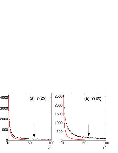
Figure 1 shows the distributions for reactions (a) and (b) , respectively compared with signal MC simulations. The accumulations at thresholds represent events satisfying momentum balance. We apply a very loose selection, , optimized using the data, and remove events consistent with being entirely due to background. We note a higher background in the data, but keep the same loose selection to achieve a similar efficiency.
Events with balanced momentum are then required to satisfy energy balance requirements. In the above decays the originating from direct / decays have a soft laboratory momentum distribution (), partially overlapping with the hard momentum distributions for the hadrons originating from the decay. We therefore require energy balance, following a combinatorial approach.
For each combination of candidates, we first require both particles to be identified loosely as pions and compute the recoiling mass
| (5) |
where is the particle four-momentum. The distribution of is expected to peak at the squared mass for signal events. Figure 2 shows the combinatorial recoiling mass for and data, where narrow peaks at the mass can be observed.
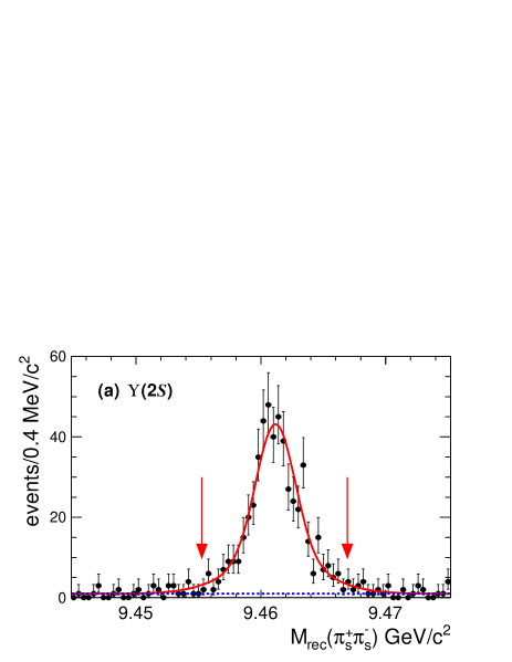
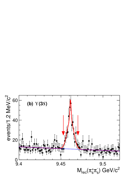
We fit each of these distributions using a linear function for the background and the sum of two Gaussian functions for the signal, obtaining average and values for the and data, respectively. We select signal event candidates by requiring
| (6) |
where indicates the fitted mass value. We obtain, in the above mass window, values of signal-to-background ratios of 517/40 and 276/150 for and data, respectively.
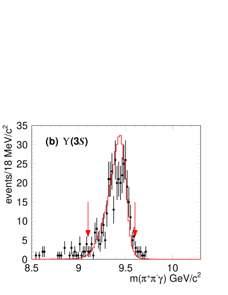
To reconstruct decays, we require a loose identification of both pions from the decay and obtain the distributions of shown in Fig. 3. The distributions show the expected peak at the mass with little background but do not have a Gaussian shape due to the asymmetric energy response of the EMC to a high-energy photon. The full line histograms compare the data with signal MC simulations and show good agreement.
We finally isolate the decay by requiring
| (7) |
At this stage no more than one candidate per event is present.
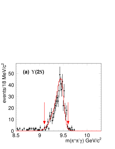
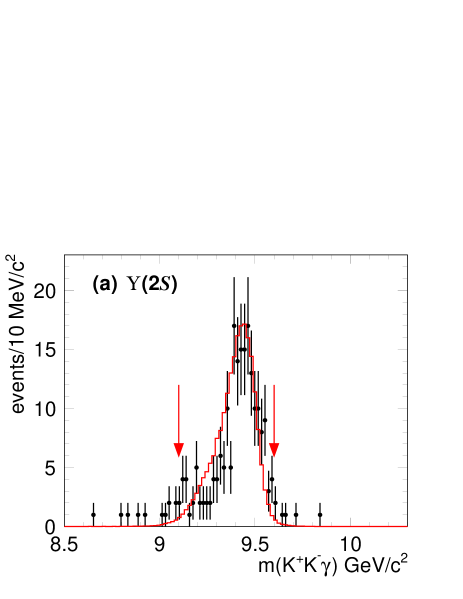
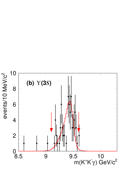
We reconstruct the final state where in a similar manner, by applying a loose identification of both kaons in the final state and requiring the mass, shown in Fig. 4, to be in the range
| (8) |
IV Study of the and mass spectra
The mass spectrum, for and summed over the and datasets with 507 and 277 events, respectively, is shown in Fig. 5(a). The resulting mass spectrum, summed over the and datasets with 164 and 63 events, respectively, is shown in Fig. 5(b). For a better comparison the two distributions are plotted using the same bin size and the same mass range.
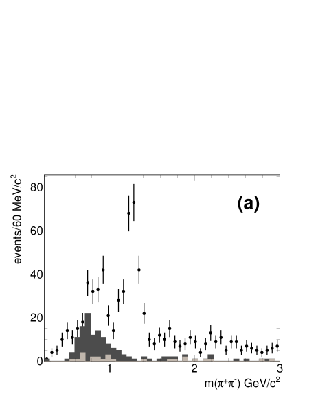
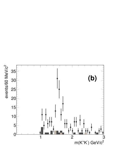
We study the background for both and final states using the sidebands. We select events in the regions on both sides of the signal region and require the and to be in the ranges defined by Eq. 7 and Eq. 8, respectively. The resulting and mass spectra for these events are superimposed in gray in Fig. 5(a) and Fig. 5(b), respectively. We note rather low background levels for all the final states, except for the mass spectrum from the data, which shows an enhancement at a mass of 750 , which we attribute to the presence of background. The mass spectrum from inclusive decays also shows a strong contribution.
We search for background originating from a possible hadronic decay, where one of the two ’s from the decay is lost. For this purpose, we make use of the data and select events having four charged pions and only one candidate. We then select events satisfying Eq. (6) and plot the effective mass distribution. No signal is observed, which indicates that the branching fraction for this possible decay mode is very small and therefore that no contamination is expected in the study of the decay mode.
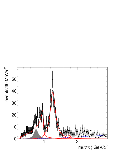
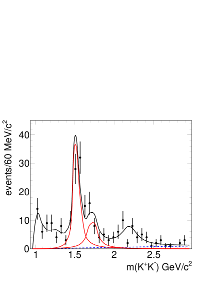
The mass spectrum, in 30 bin size is shown in Fig. 6. The spectrum shows , resonance production, with low backgrounds above 1 . We observe a rapid drop around 1 characteristic of the presence of the , and a strong signal. The data also suggest the presence of weaker resonant contributions. The mass spectrum is shown in Fig. 7 and also shows resonant production, with low background. Signals at the positions of and can be observed.
We make use of a phenomenological model to extract the different branching fractions, where is an intermediate resonance.
IV.1 Fit to the mass spectrum
We perform a simultaneous binned fit to the mass spectra from the and datasets using the following model.
| Resonances () | Yield | Yield | Significance |
|---|---|---|---|
| -wave | 12.8 | ||
| 15.9 | |||
| 2.5 | |||
| 54 23 | |||
| Resonances () | Yield + | Significance | |
| 5.6 | |||
| 8.9 | |||
| 4.7 | |||
-
•
We describe the low-mass region (around the ) using a relativistic -wave Breit-Wigner lineshape having free parameters. We test the -wave hypothesis in Sec.VI and Sec.VIII. We obtain its parameters from the data only, and we fix them in the description of the data.
-
•
We describe the using the Flatté flatte formalism. For the channel the Breit-Wigner lineshape has the form
(9) and in the channel the Breit-Wigner function has the form
(10) where is absorbed into the intensity of the resonance. and describe the partial widths of the resonance to decay to and and are given by
(11) where and are the squares of the coupling constants of the resonance to the and systems. The parameters and couplings are taken from Ref. Armstrong : , and .
-
•
The total -wave is described by a coherent sum of and as
(12) where and are free parameters for the relative intensity and phase of the two interfering contributions.
-
•
The and resonances are represented by relativistic Breit-Wigner functions with parameters fixed to PDG values PDG .
-
•
In the high mass region we are unable, with the present statistics, to distinguish the different possible resonant contributions. Therefore we make use of the method used by CLEO Dobbs and include a single resonance having a width fixed to the PDG value () and unconstrained mass.
-
•
The background is parametrized with a quadratic dependence
where is the center-of-mass momentum in the rest frame, which goes to zero at threshold.
-
•
For the data we also include background with parameters fixed to the PDG values.
The fit is shown in Fig. 6. It has 16 free parameters and for ndf=152, corresponding to a -value of 5%. The yields and statistical significances are reported in Table 1. Significances are computed as follows: for each resonant contribution (with fixed parameters) we set the yield to zero and compute the significance as , where is the difference in between the fit with and without the presence of the resonance.
The table also reports systematic uncertainties on the yields, evaluated as follows: the parameters of each resonance are modified according to , where is the PDG uncertainty and the deviations from the reference fit are added in quadrature. The background has been modified to have a linear shape. The effective range in the Blatt-Weisskopf blatt factors entering in the description of the intensity and the width of the relativistic Breit-Wigner function have been varied between 1 and 5 , and the average deviation is taken as a systematic uncertainty. The different contributions, dominated by the uncertainties on the resonances parameters, are added in quadrature.
We note the observation of a significant -wave in radiative decays. This observation was not possible in the study of radiative decay to because of the presence of a strong, irreducible background from pipi_markiii . We obtain the following parameters:
| (13) |
and rad. The fraction of -wave events associated with the is . We also obtain .
IV.2 Study of the mass spectrum.
Due to the limited statistics we do not separate the data into the and datasets. We perform a binned fit to the combined mass spectrum using the following model:
-
•
The background is parametrized with a linear dependence starting with zero at threshold.
-
•
The is parametrized according to the Flatté formalism described by Eq. (10) for the projection.
-
•
The , , , and resonances are represented by relativistic Breit-Wigner functions with parameters fixed to PDG values.
-
•
We include an contribution having parameters fixed to the PDG values.
The fit shown in Fig. 7. It has six free parameters and for ndf=29, corresponding to a -value of 20%; the yields and significances are reported in Table 1. Systematic uncertainties have been evaluated as for the fit to the mass spectrum. The parameters of each resonance are modified according to , where is the PDG uncertainty and the deviations from the reference fit are added in quadrature. The background has been modified to have a quadratic shape. The effective range in the Blatt-Weisskopf blatt factors entering in the description of the intensity and the width of the relativistic Breit-Wigner function have been varied between 1 and 5 , and the average deviation is taken as a systematic uncertainty. The different contributions, dominated by the uncertainties on the resonances parameters, are added in quadrature. In the 1500 mass region both and can contribute, therefore we first fit the mass spectrum assuming the presence of only and then replace in the fit the with the resonance. In Table 1 we label this contribution as . The resulting yield variation between the two fits is small and gives a negligible contribution to the total systematic uncertainty. A separation of the and contributions is discussed in Secs. VI and VII.
V Efficiency correction
V.1 Reconstruction efficiency
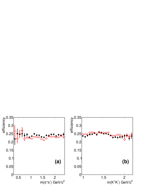
To compute the efficiency, MC signal events are generated using a detailed detector simulation geant . These simulated events are reconstructed and analyzed in the same manner as data. The efficiency is computed as the ratio between reconstructed and generated events. The efficiency distributions as functions of mass, for the / data and for the and final states, are shown in fig. 8. We observe an almost uniform behavior for all the final states.
We define the helicity angle as the angle formed by the (where ), in the rest frame, and the in the rest frame. We also define as the angle formed by the radiative photon in the rest frame with respect to the direction in the / rest frame.
We compute the efficiency in two different ways.
-
•
We label with the efficiency computed as a function of the effective mass and the helicity angle . This is used only to obtain efficiency-corrected mass spectra.
-
•
We label with the efficiency computed, for each resonance mass window (defined in Table 3), as a function of and . This is used to obtain the efficiency-corrected angular distributions and branching fractions of the different resonances.
To smoothen statistical fluctuations in the evaluation of , for , we divide the mass into nine 300--wide intervals and plot the in each interval. The distributions of are then fitted using cubic splines spline . The efficiency at each is then computed using a linear interpolation between adjacent bins.
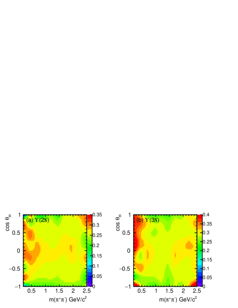
Figure 9 shows the efficiency distributions in the (, ) plane for the and datasets. We observe an almost uniform behavior with some loss at close to . The efficiencies integrated over are consistent with being constant with mass and have average values of and .
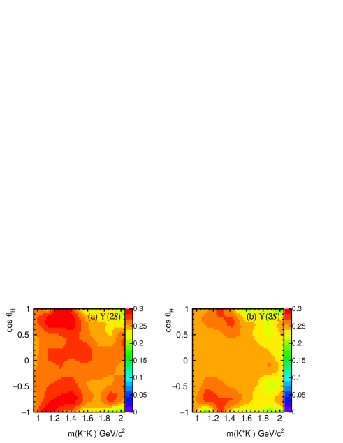
A similar method is used to compute for the final state. The average efficiency values are and . Figure 10 shows the efficiency distributions in the (, ) plane for the and datasets.
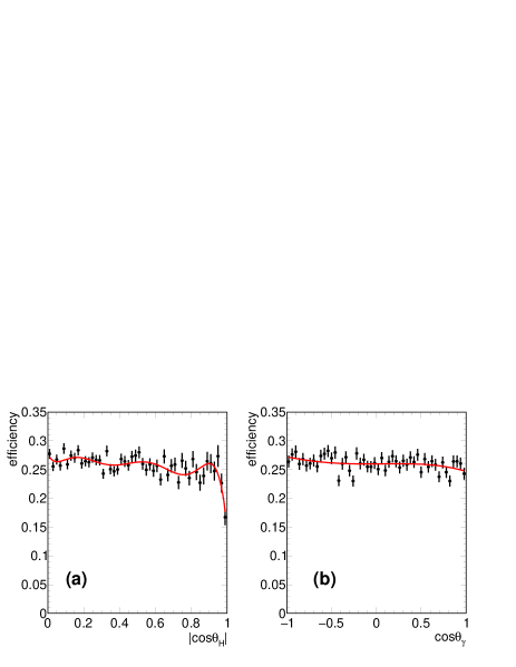
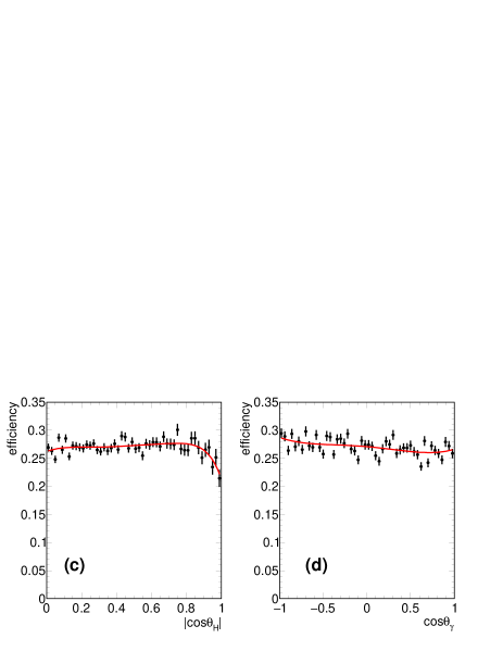
We also compute the efficiency in the plane for each considered resonance decaying to and . Since there are no correlations between these two variables, we parametrize the efficiency as
| (14) |
The distributions of the efficiencies as functions of and are shown in Fig. 11 for the and mass regions, for the datasets. To smoothen statistical fluctuations, the efficiency projections are fitted using 7-th and 4-th order polynomials, respectively. Similar behavior is observed for the other resonances and for the datasets.
| Resonance | ||||
|---|---|---|---|---|
| corrected yield | corrected yield | |||
| -wave | ||||
| Resonance | / | / | ||
| corrected yield | ||||
V.2 Efficiency correction
To obtain the efficiency correction weight for the resonance we divide each event by the efficiency
| (15) |
where is the number of events in the resonance mass range. The resulting efficiency weight for each resonance is reported in Table 2. We compute separately the and yields for resonances decaying to while, due to the limited statistics, for resonances decaying to the two datasets are merged and corrected using the weighted average efficiency. The systematic effect related to the effect of particle identification is assessed by the use of high statistics control samples. We assign systematic uncertainties of 0.2% to the identification of each pion and 1.0% to that of each kaon. We include an efficiency correction of to the reconstruction of the high energy photon, obtained from studies on Data/MC detection efficiency. The efficiency correction contribution due to the limited MC statistics is included using the statistical uncertainty on the average efficiency weight as well as the effect of the fitting procedure. The above effects are added in quadrature and are presented in Table 2 as systematic uncertainties related to the efficiency correction weight. Finally we propagate the systematic effect on event yields obtained from the fits to the mass spectra. The resulting efficiency corrected yields are reported in Table 2.
VI Legendre Polynomial Moments analysis
To obtain information on the angular momentum structure of the and systems in we study the dependence of the mass on the helicity angle . Figure 12 shows the scatter plot vs for the combined and datasets. We observe the spin 2 structure of the .
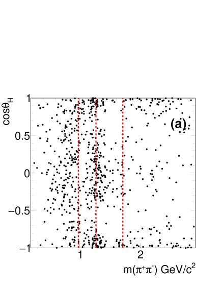
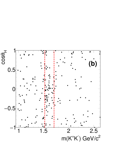
A better way to observe angular effects is to plot the mass spectrum weighted by the Legendre polynomial moments, corrected for efficiency. In a simplified environment, the moments are related to the spin 0 () and spin 2 () amplitudes by the equations costa :
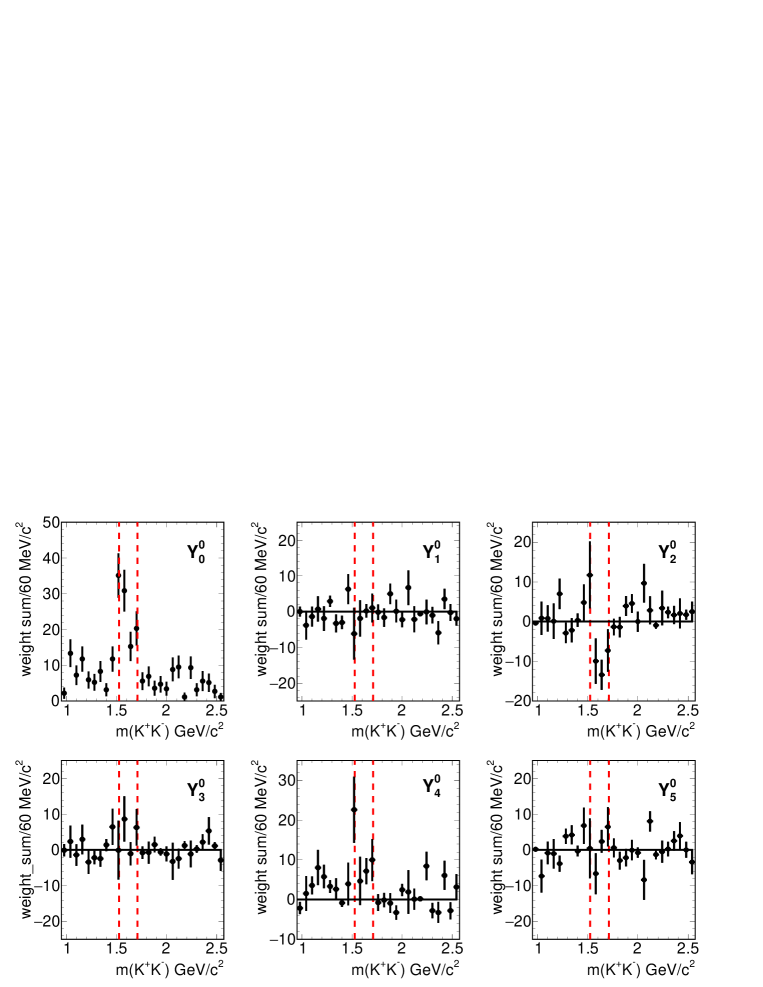
| (16) |
where is the relative phase. Therefore we expect to observe spin 2 resonances in and interference in . The results are shown in Fig. 13. We clearly observe the resonance in and a sharp drop in at the mass, indicating the interference effect. The distribution of is just the scaled mass distribution, corrected for efficiency. Odd moments are sensitive to the forward-backward asymmetry and show weak activity at the position of the mass. Higher moments are all consistent with zero.
Similarly, we plot in Fig. 14 the mass spectrum weighted by the Legendre polynomial moments, corrected for efficiency. We observe signals of the and in and activity due to interference effects in the moment. Higher moments are all consistent with zero.
Resonance angular distributions in radiative decays from / decays are rather complex and will be studied in Sec.VIII. In this section we perform a simplified Partial Wave Analysis (PWA) solving directly the system of Eq. (16). Figure 15 and Fig. 16 show the resulting -wave and -wave contributions to the and mass spectra, respectively. Due to the presence of background in the threshold region, the analysis is performed only on the data. The relative phase is not plotted because it is affected by very large statistical errors.
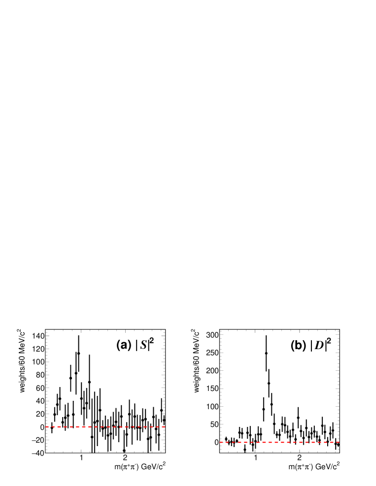
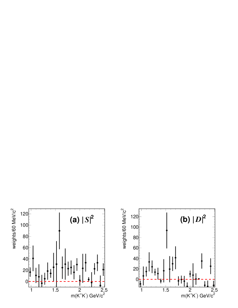
We note that in the case of the mass spectrum we obtain a good separation between and -waves, with the presence of an resonance on top of a broad resonance in the -wave and a clean in the -wave distribution. Integrating the -wave amplitude from threshold up to a mass of 1.5 , we obtain an integrated, efficiency corrected yield
| (17) |
in agreement with the results from the fit to the mass spectrum (see Table 2). We also compute the fraction of -wave contribution in the mass region defined in Table 3 and obtain .
In the case of the PWA the structure peaking around 1500 appears in both and -waves suggesting the presence of and . In the mass region there is not enough data to discriminate between the two different spin assignments. This pattern is similar to that observed in the Dalitz plot analysis of charmless decays fx . Integrating the and -wave contributions in the mass region in the range given in Table 3, we obtain a fraction of -wave contribution .
VII Spin-parity analysis
We compute the helicity angle defined as the angle formed by the , in the rest frame, with respect to the direction of the system in the rest frame. This distribution is shown in Fig. 17 for the data and , and is expected to be uniform if is an -wave system. The distribution is consistent with this hypothesis with a -value of 65%.
The angular distributions are expressed in terms of and . Due to the decay chain used to isolate the radiative decays (see Eq. (1) and Eq. (2)), the can be produced with helicity 0 or 1 and the corresponding amplitudes are labeled as and , respectively. A spin 2 resonance, on the other hand, can have three helicity states, described by amplitudes , , and . We make use of the helicity formalism cleothesis ; richman to derive the angular distribution for a spin 2 resonance:
| (18) | |||||
Ignoring the normalization factor , there are two amplitudes describing the helicity states, which can be reduced to one free parameter by taking the ratio . Similarly, the three amplitudes describing the spin 2 helicity states, can be reduced to two free parameters by taking the ratios and . We therefore have a total of three free parameters.
The expected angular distribution for a spin 0 resonance is given by
| (19) |
Ignoring the normalization factors and , the distribution has only one free parameter, .
We perform a 2D unbinned maximum likelihood fit for each resonance region defined in Table 3. If is the number of available events, the likelihood function is written as:
| (20) |
where is the signal fraction, is the fitted efficiency (Eq. (14)), and and are the functions describing signal and background contributions, given by Eq. (18) or Eq. (19). Since the background under the and mass spectra is negligible in the low-mass regions, we include only the tails of nearby adjacent resonances. In the description of the data in the threshold region we make use only of the data because of the presence of a sizeable background in the sample.
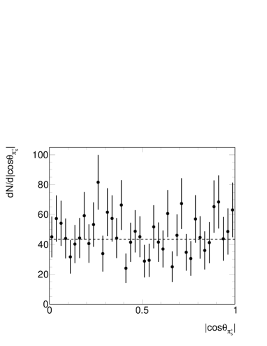
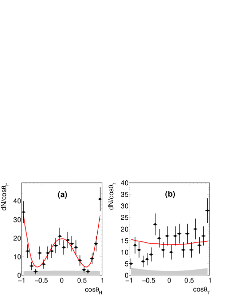
We first fit the angular distributions and allow a background contribution of 16% (see Sect. VII) from the -wave having fixed parameters. Therefore an iterative procedure of fitting the -wave and regions is performed. Figure 18 shows the uncorrected fit projections on and . The spectrum is approximately uniform, while shows structures well-fitted by the spin 2 hypothesis. Table 3 summarizes the results from the fits. We use as figures of merit , and their sum computed as the values obtained from the and projections, respectively. We use , where is the number of free parameters in the fit and is the sum of the number of bins along the and axes. We note a good description of the projection but a poor description of the projection. This may be due to the possible presence of additional scalar components in the mass region, not taken into account in the formalism used in this analysis.
| Resonance | mass range () | events | spin | , , | |||
| -wave | 0.6-1.0 | 104 | 0 | 5.8, 8.4, 14.3/19 | 0.09 0.33 | ||
| 1.092-1.460 | 280 | 2 | 24.0, 46.0, 70/37 | 1.07 0.31 | 0.00 0.03 | 0.29 0.08 | |
| 1.424-1.620 | 36 | 2 | 6.7, 1.8, 8.5/16 | ||||
| 40 | 0 |
We fit the -wave region in the mass spectrum from the decay including as background the spin 2 contribution due to the tail of the . The latter is estimated to contribute with a fraction of 9%, with parameters fixed to those obtained from the spin analysis described above. Figure 19 shows the fit projections on the and distributions and Table 3 gives details on the fitted parameters. We obtain a good description of the data consistent with the spin 0 hypothesis.
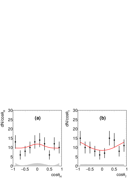
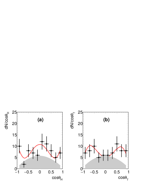
We fit the data in the mass region, where many resonances can contribute: , fx , and . We fit the data using a superposition of and waves, having helicity contributions as free parameters, and free -wave contribution. We obtain an -wave contribution of , in agreement with the estimate obtained in Sec.VI. The helicity contributions are given in Table 3 and fit projections are shown in Fig. 20, giving an adequate description of the data. We assign the spin-2 contribution to the and the spin-0 contribution to the resonance. We also fit the data assuming the presence of the spin-2 only hypothesis. We obtain a likelihood variation of for the difference of two parameters between the two fits. Due the low statistics we cannot statistically distinguish between the two hypotheses.
VIII Measurement of branching fractions
We determine the branching fraction for the decay of to photon and resonance using the expression
| (21) | |||||
where indicates the efficiency-corrected yield for the given resonance. To reduce systematic uncertainties, we first compute the relative branching fraction to the reference channel , which has the same number of charged particles as the final states under study. We then multiply the relative branching fraction by the well-measured branching fraction % PDG .
We determine the reference channel corrected yield using the method of “-counting”, also used to obtain the number of produced and book . Taking into account the known branching fractions of we obtain
| (22) |
and
| (23) |
events. As a cross-check we reconstruct corrected for efficiency and obtain yields in good agreement with those obtained using the method of “-counting”.
Table 4 gives the measured branching fractions. In all cases we correct the efficiency corrected yields for isospin and for PDG measured branching fractions PDG . In these measurements the yield is corrected first for the (33.3%) and then for the () branching fractions. We also correct the -wave and branching fractions for the decay mode. In the case of the spin analysis reported in Sec.VI and Sec.VII gives indications of the presence of overlapping and contributions. We give the branching fraction for and, separately, for the and , where we make use of the -wave contribution , obtained in Sec.VII.
The branching fraction is corrected for the decay mode (). For all the resonances decaying to , the branching fractions are corrected for the unseen decay mode (50%).
For the and resonances decaying to , the relative branching ratios are computed separately for the and datasets, obtaining good agreement. The values reported in Table 4 are determined using the weighted mean of the two measurements.
| Resonance | () |
|---|---|
| -wave | |
Since the reference channel has the same number of tracks as the final state, systematic uncertainties related to tracking are negligible with respect to the errors due to other sources. The systematic uncertainty related to the “-counting” estimate of the event yields in the denominator of Eq. 21 is propagated into the total systematic uncertainty on the branching fractions given in Table 4.
Comparing with CLEO results, we note that our results on the -wave contribution include the and contributions, while the CLEO analysis determines the branching fraction for the peaking structure at the mass. In the same way a direct comparison for the branching fraction is not possible due to the contribution included in the present analysis. The branching fraction for the is in good agreement.
We report the first observation of in radiative decay with a significance of , combining and data. To determine the branching ratio of the decays to and , we remove all the systematic uncertainties related to the reference channels and of the reconstruction. Labeling with the efficiency-corrected yields for the two decay modes, we obtain
| (24) | |||||
in agreement with the world average value of PDG .
IX Summary
We have studied the radiative decays to and using data recorded with the BABAR detector operating at the SLAC PEP-II asymmetric-energy collider at center-of-mass energies at the and resonances, using integrated luminosities of 13.6 and 28.0 , respectively. The resonance is reconstructed from the decay chains , . Spin-parity analyses and branching fraction measurements are reported for the resonances observed in the and mass spectra. In particular, we report the observation of broad -wave, , and resonances in the mass spectrum. We observe a signal in the 1500 mass region of the mass spectrum for which the spin analysis indicates contributions from both and resonances. We also report observation of in both and mass spectra with combined significance of , and measure the relative branching fraction. These results may contribute to the long-standing issue of the identification of a scalar glueball.
Reference ochs reports on a detailed discussion on the status of the search for the scalar glueball, listing as candidates the broad , , , and . For this latter state, in the gluonium hypothesis, Ref. zhu computes a branching fraction of . Taking into account the presence of additional, not well measured, decay modes, our result is consistent with this predicted branching fraction as well as with the dominance of an decay mode. For , ref. he expects a branching fraction in the range , consistent with our measurement. The status of is controversial pdg2006 as this state could just be an effect related to the broad . Reference zhu estimates for a branching fraction of , in the range of our measurement of the branching fraction of .
X Acknowledgments
We are grateful for the extraordinary contributions of our PEP-II colleagues in achieving the excellent luminosity and machine conditions that have made this work possible. The success of this project also relies critically on the expertise and dedication of the computing organizations that support BABAR. The collaborating institutions wish to thank SLAC for its support and the kind hospitality extended to them. This work is supported by the US Department of Energy and National Science Foundation, the Natural Sciences and Engineering Research Council (Canada), the Commissariat à l’Energie Atomique and Institut National de Physique Nucléaire et de Physique des Particules (France), the Bundesministerium für Bildung und Forschung and Deutsche Forschungsgemeinschaft (Germany), the Istituto Nazionale di Fisica Nucleare (Italy), the Foundation for Fundamental Research on Matter (The Netherlands), the Research Council of Norway, the Ministry of Education and Science of the Russian Federation, Ministerio de Economia y Competitividad (Spain), and the Science and Technology Facilities Council (United Kingdom). Individuals have received support from the Marie-Curie IEF program (European Union), the A. P. Sloan Foundation (USA) and the Binational Science Foundation (USA-Israel). We acknowledge P. Colangelo for useful suggestions.
References
- (1) Y. Chen et al. Phys. Rev. D 73, 014516 (2006).
- (2) E. Klempt and A. Zaitsev, Phys. Rept. 454, 1 (2007).
- (3) W. Ochs, J. Phys. G 40, 043001 (2013).
- (4) P. Minkowski and W. Ochs, Eur. Phys. J. C 9, 283 (1999).
- (5) C. Amsler and F.E. Close, Phys. Lett. B 353, 385 (1995).
- (6) C. Amsler and F.E. Close, Phys.Rev. D 53, 295 (1996).
- (7) S. Janowski, F. Giacosa and D. H. Rischke, Phys. Rev. D 90, 114005 (2014).
- (8) M. Chanowitz, Phys. Rev. Lett. 95, 172001 (2005).
- (9) K. Ta. Chao, X. G. He and J. P. Ma, Phys. Rev. Lett. 98, 149103 (2007).
- (10) R. Zhu, JHEP 1509, 166 (2015).
- (11) S. Fleming and A. K. Leibovich, Phys. Rev. D 70, 094016 (2004).
- (12) S. Fleming, C. Lee and A. K. Leibovich, Phys. Rev. D 71, 074002 (2005).
- (13) X. G. He, H. Y. Jin and J. P. Ma, Phys. Rev. D 66, 074015 (2002).
- (14) L. Köpke and N. Wermes, Phys. Rept. 174, 67 (1989).
- (15) J. Z. Bai et al. (BES Collaboration), Phys. Rev. Lett. 77, 3959 (1996).
- (16) J. Z. Bai et al. (BES Collaboration), Phys. Rev. D 67, 032004 (2003).
- (17) S.B. Athar et al. (CLEO Collaboration), Phys. Rev. D 73, 032001 (2006).
- (18) D. Besson et al. (CLEO Collaboration), Phys. Rev. D 75, 072001 (2007).
- (19) J.P. Lees et al. (BABAR Collaboration), Nucl. Instr. Meth. Phys. Res. A 726, 203 (2013).
- (20) B. Aubert et al. (BABAR Collaboration), Nucl. Instr. Meth. Phys. Res. A 479, 1 (2002); ibid. 729, 615 (2013).
- (21) The BABAR detector Monte Carlo simulation is based on Geant4 [S. Agostinelli et al., Nucl. Instr. Meth. Phys. Res. A 506, 250 (2003)] and EvtGen [D. J. Lange, Nucl. Instr. Meth. Phys. Res. A 462, 152 (2001)].
- (22) Ed. A.J. Bevan, B. Golob, Th. Mannel, S. Prell, and B.D. Yabsley, “The Physics of the B Factories”, Eur. Phys. J. C 74, 3026 (2014).
- (23) S.M. Flatté, Phys. Lett. B 63, 224 (1976).
- (24) T.A. Armstrong et al. (WA76 Collaboration), Z. Phys. C 51, 351 (1991).
- (25) C. Patrignani et al. (Particle Data Group), Chin. Phys. C 40, 100001 (2016).
- (26) S. Dobbs, A. Tomaradze, T. Xiao, and K.K. Seth, Phys. Rev. D 91, 052006 (2015).
- (27) J. Blatt and V. Weisskopf, Theoretical Nuclear Physics, New York: John Wiley & Sons (1952).
- (28) R. M. Baltrusaitis et al. (Mark III Collaboration), Phys. Rev. D 35, 2077 (1987).
- (29) C. De Boor, “A practical guide to splines”; rev. ed. Springer (2001).
- (30) G. Costa et al. Nucl. Phys. B175 402 (1980).
- (31) J.P. Lees et al. (BABAR Collaboration), Phys.Rev. D 85, 112010 (2012).
- (32) L. Breva-Newell, “Decays of the into a photon and two charged hadrons”, PhD thesis, hep-ex/0412075 (2004).
- (33) J.D. Richman, “An Experimenter’s Guide to the Helicity Formalism”, CALT-68-1148 (1984).
- (34) W. M. Yao et al. (Particle Data Group), J. Phys. G 33, 1 (2006).