Reproducing the Kolmogorov spectrum of turbulence with a hierarchical linear cascade model

Abstract

In Richardson’s cascade description of turbulence, large vortices break up to form smaller ones, transferring the kinetic energy towards smaller scales. Energy dissipation occurs at the smallest scales due to viscosity. We study this energy cascade in a phenomenological model of vortex breakdown. The model is a binary tree of decreasing masses connected by softening springs, with dampers acting on the lowest level. The masses and stiffnesses between levels change according to a power law. The different levels represent different scales, enabling the definition of “mass wavenumbers”. The eigenvalue distribution of the model exhibits a devil’s staircase self-similarity. The energy spectrum of the model (defined as the energy distribution among the different mass wavenumber) is derived in the asymptotic limit. A decimation procedure is applied to replace the model with an equivalent chain oscillator. For a range of stiffness parameter the energy spectrum is qualitatively similar to the Kolmogorov spectrum of 3D homogeneous, isotropic turbulence and we find the stiffness parameter for which the energy spectrum has the well-known $-5/3$ scaling exponent.

1 Introduction

Many natural phenomena and engineering processes exhibit energy transfer among a range of different scales. Frequently studied examples include nonlinear chain oscillators [1, 2, 3, 4]. Direct energy cascade describes primary energy transfer from large scales to small ones, while inverse cascade [5] refers to energy transfer from small scales towards larger ones. Turbulent flow is a prime example of a process which exhibits different scales and an energy cascade. Richardson’s so-called ”eddy hypothesis” [6, 7] argues that the largest eddies are unstable and break up forming several smaller vortices, gradually transferring the kinetic energy of the flow to smaller scales.

The turbulent energy cascade is characterized by the energy spectrum $\hat{E}(\kappa)$ which describes the distribution of the total energy

$$E=\int\hat{E}(\kappa)d\kappa.$$ (1)

among the different scales. The wavenumber $\kappa\sim 1/L$ is associated with the vortex having characteristic size $L$. In Figure 1 the so-called Kolmogorov spectrum of 3D homogeneous isotropic turbulence is shown, illustrating the main features of the turbulent energy cascade [8, 9, 10]. The Kolmogorov length scale is denoted with $\eta$.

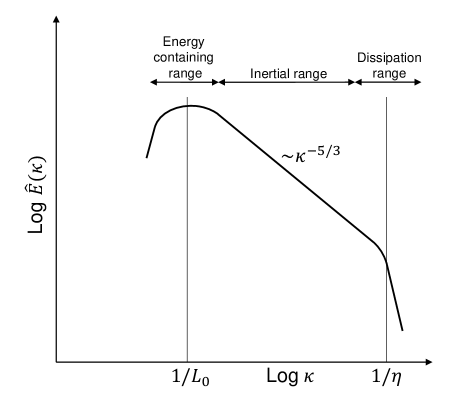
Figure 1: Qualitative graph of the Kolmogorov spectrum.

The energy production mainly affects the large scales (characterized by $L_{0}$), hence the bulk of the energy is contained in the large eddies (energy containing range). In the intermediate wavenumbers ($1/L_{0}<\kappa<1/\eta$, called the inertial range) the energy spectrum is described by the famous Kolmogorov scaling law [8, 10]

$$\hat{E}(\kappa)\sim\kappa^{-5/3}.$$ (2)

The largest wavenumbers ($\kappa>1/\eta$) are associated with length scales smaller than the Kolmogorov scale. In this dissipation range most kinetic energy is lost due to viscous friction. The Kolmogorov spectrum is confirmed by many measurements and simulations [11, 12, 13, 14].

We present a phenomenological model of turbulence inspired by Richardson’s cascade description and to demonstrate that this model exhibits the Kolmogorov spectrum for a suitably chosen parameter. The model is a binary tree of masses and springs (Figure 2(a)) in which the masses represent the different scales, and the springs are responsible for the energy transfer.

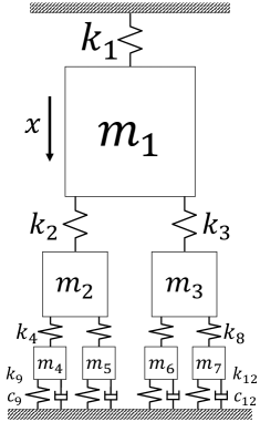
(a)

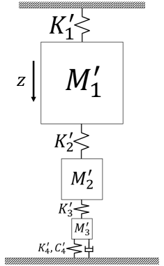
(b)

Figure 2: (a) The mechanistic model and (b) the equivalent chain oscillator.

Even though this model is linear, linear systems can also contain a wide range of scales and exhibit complex behavior [15]. In fact, nonlinear systems can be embedded in infinite-dimensional linear systems [16]. Leyden and Goodwine [17] set up a similarly structured mass-spring-damper system and showed that the infinite version of the system is described by a fractional ($1/2$th order) differential equation. Many studies aim at designing effective vibration absorbers by realizing targeted energy transfer, a primarily one-way energy transfer from the primary system to the dissipative element. Tripathi et al. [18] investigated and compared the performance of a nonlinear energy sink (a light mass with viscous damping and an essentially nonlinear spring) and linear tuned mass damper on multi-degree-of-freedom systems. Pumhössel found a method to effectively transfer energy among vibration modes using impulsive force excitations [19].

2 Mechanistic turbulence model

Our mechanistic turbulence model is an $n$-level binary tree of masses and springs, with dampers at the ground level (Figure 2(a) shows a $3$-level model). Level $l\in\left\{1,...,n\right\}$ consists of $2^{l-1}$ masses, the total number of masses is $N=2^{n}-1$. The top mass is connected to the rigid ceiling with a spring, while the bottom masses are connected to the rigid ground with springs and dampers (signifying dissipation only at the lowest scale). Every mass $m_{i}$ ($i=1,...N$) has a parent and two (left and right) children whose indices are ($\lfloor.\rfloor$ denotes the floor operation)

$$\mathcal{P}(i)=\lfloor i/2\rfloor,\quad\mathcal{L}(i)=2i,\quad\mathcal{R}(i)=2i+1,\quad i=1,...N.$$ (3)

The equations of motion are

$$\begin{split}m_{i}\ddot{x}_{i}=&k_{i}(x_{\mathcal{P}(i)}-x_{i})+k_{\mathcal{L}(i)}(x_{\mathcal{L}(i)}-x_{i})+k_{\mathcal{R}(i)}(x_{\mathcal{R}(i)}-x_{i})+\\ &+c_{i}\left(\dot{x}_{\mathcal{P}(i)}-\dot{x}_{i}\right)+c_{\mathcal{L}(i)}(\dot{x}_{\mathcal{L}(i)}-\dot{x}_{i})+c_{\mathcal{R}(i)}(\dot{x}_{\mathcal{R}(i)}-\dot{x}_{i}),\quad i=1,...,N,\end{split}$$ (4)

with the boundary conditions (the ceiling and the ground are motionless)

$$x_{i}=0,\quad i=0,N+1,...,2N+1.$$ (5)

The initial conditions are

$$x_{i}(0)=x_{i,0},\ \dot{x}_{i}(0)=v_{i,0},\quad i=1,...,N.$$ (6)

Eqs. (4) and (6) in matrix form is

$$\mathcal{M}\ddot{\mathbf{x}}+\mathcal{C}\dot{\mathbf{x}}+\mathcal{K}\mathbf{x}=\mathbf{0},\quad\mathbf{x}(0)=\mathbf{x}_{0},\quad\mathbf{\dot{x}}(0)=\mathbf{v}_{0},$$ (7)

where $\mathbf{x}$ is the vector of displacements, $\mathcal{M}$, $\mathcal{C}$, $\mathcal{K}$ are the mass, damping, and stiffness matrices, respectively.

2.1 Model parameters

We introduce a quantity analogous with the wavenumber of a turbulent scale, the “mass wavenumber”

$$\kappa_{l}=1/M_{l},\quad l=1,...,n.$$ (8)

Here $M_{l}$ is the mass scale representing masses in level $l$ (average, for example). For the ease of exposition we set every mass, stiffness and damping coefficient equal within a level $l$ and denote these with $M_{l}$, $K_{l}$, $C_{l}$. To represent different scales, the masses are gradually decreased in lower levels, analogously to the eddy hypothesis, in which a large vortex breaks up into smaller ones.

The mass scale $M_{l}$ is specified by the power-law distribution

$$M_{l}=\left(\frac{1}{2}\right)^{l-1},\quad l=1,...,n,$$ (9)

thus the sum of masses in each level is 1. Similarly, we denote by $K_{l}$ the stiffness coefficient of the springs connecting the masses of the $l-1$th and $l$th levels. The $K_{l}$ values are also specified with a power-law distribution with base $\sigma>0$ (stiffness parameter), i.e.

$$K_{l}=\sigma^{l-1},\quad l=1,...,n+1.$$ (10)

By design, we only have dampers between the bottom masses and the rigid ground, hence only $C_{n+1}$ is nonzero and we set

$$C_{n+1}=2\sqrt{M_{n}K_{n+1}}=2^{\frac{3-n}{2}}\sigma^{\frac{n}{2}}.$$ (11)

The characteristics of the energy spectrum of the model (defined in Section 4) of course depends on the relation between the base parameters of Eqs. (9) and (10) ($1/2$ and $\sigma$). This means that one such base parameter is enough to describe the behavior of the mechanistic model. This is why the base of the mass distribution was set to $1/2$. Furthermore, based on our experience the energy spectrum is practically independent of the damping.

3 The eigenvalue distribution of the mechanistic model

The eigenvalues of system (7) are the roots of the characteristic equation

$$P(\lambda)=\det(\mathcal{M}\lambda^{2}+\mathcal{C}\lambda+\mathcal{K})=0.$$ (12)

Figure 3 shows the histogram and the eigenvalue distribution of the purely imaginary eigenvalues of system (7) for the undamped ($\mathcal{C}=0$) case with 8-levels, $\sigma=1/2$.

(a)

(b)

Figure 3: (a) Histogram and (b) eigenvalue distribution of the conservative 8-level mechanistic model for $\sigma=1/2$.

The eigenvalue distribution shown in Figure 3(b) exhibits a “devil’s staircase” type self-similarity. He et al. [20] demonstrated that the adjacency matrix for a class of symmetric tree graphs have devil’s staircase type spectrum. Kalmár-Nagy et al. [21] showed the same for a different type of self-similar graph, as well as that the characteristic polynomial of the adjacency matrix of such a graph is a product of Chebyshev polynomials.

Claim 1.

The characteristic polynomial (12) of the undamped system (Eq. (7) with $\mathcal{C}=0$) with parameter $\sigma=1/2$ has the form

$$P_{0}(\lambda)=1,\quad P_{n}(\lambda)=\frac{Q_{n}(\lambda)}{Q_{n-1}(\lambda)}P_{n-1}^{2}(\lambda)=Q_{n}(\lambda)\prod_{i=0}^{n-1}Q_{i}(\lambda)^{2^{n-(i+1)}},\quad n>0.$$ (13)

Here $Q_{i}(\lambda)$ are generalized Chebyshev-polynomials of the second kind given by

$$Q_{0}(\lambda)=1,\quad Q_{i}(\lambda)=U_{i}\left(\frac{\lambda^{2}+2}{2}\right)-\frac{1}{2}U_{i-1}\left(\frac{\lambda^{2}+2}{2}\right),\quad i>0,$$ (14)

and $U_{i}$ denotes the $i$th Chebyshev-polynomial of the second kind [22].

Figure 4 shows the eigenvalue distributions of the imaginary parts of the complex eigenvalues for damped 8-level systems.

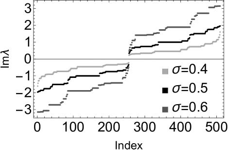
Figure 4: The distribution of $\text{Im}\lambda$ of 8-level damped mechanistic models for different $\sigma$ values.

These distributions still exhibit similar characteristics as Figure 3.

4 The energy spectrum of the mechanistic model

For turbulent flows the energy spectrum $E(\kappa)$ shows the “contribution” of the different scales of eddies to the total energy of the flow, i.e. the mean energy stored in the different wavenumbers $\kappa$. An analogous energy spectrum is now defined for the mechanistic model showing the energy fraction stored in the different scales ($M_{l}$) of the system. A consequence of the finite sized mechanistic turbulence model is that its energy spectrum is discrete, as opposed to the continuous Kolmogorov spectrum of turbulence.

The total mechanical energy $E(t)$ of the system is the sum of the total kinetic energy of the masses and the total potential energy stored in the springs, i.e.

$$E(t)=\frac{1}{2}\dot{\mathbf{x}}^{T}(t)\mathcal{M}\dot{\mathbf{x}}(t)+\frac{1}{2}\mathbf{x}^{T}(t)\mathcal{K}\mathbf{x}(t).$$ (15)

The total energy is simply the sum of level energies, i.e. $E(t)=\sum_{l=1}^{n}E_{l}(t)$, where $E_{l}(t)$ is defined so that the potential energy of the springs connecting two masses are distributed equally between the two levels and the potential energy of the top spring and the bottom springs are added to $E_{1}(t)$ and $E_{n}(t)$, respectively:

$$\begin{split}E_{l}(t)=\frac{1}{2}M_{l}\sum\limits_{i\in I(l)}\dot{x}_{i}^{2}&+\frac{1}{4}(1+\delta_{l,1})K_{l}\sum\limits_{i\in I(l)}{(x_{i}-x_{\mathcal{P}(i)})^{2}}+\\ &+\frac{1}{4}(1+\delta_{l,n})K_{l+1}\sum\limits_{i\in I(l+1)}{(x_{i}-x_{\mathcal{P}(i)})^{2}},\quad l=1,...,n.\end{split}$$ (16)

Here $I(l)=\{2^{l-1},...,2^{l}-1\}$ are the indices on level $l$ and $\delta$ is the Kronecker-delta ($\delta_{i,j}=1$ for $i=j$, $0$ otherwise). This definition of $E_{l}(t)$ ensures its non-negativity for $t\geq 0$.

Figure 5 shows the total energy and the energy of the 2nd and 4th levels of an 8-level mechanistic model with $\sigma=1/2$ (launched from random initial conditions).

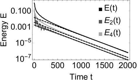
(a)

(b)

Figure 5: (a) The total energy and the energy of the 2nd and 4th levels of an 8-level mechanistic model with $\sigma=1/2$. (b) The total energy plotted for a narrow time interval.

The behavior of the energies $E(t),E_{l}(t)$ ($l=1,...,n$) consists of a transient part and a decaying oscillatory state (the dashed lines in Figure 5 are exponentially decaying functions with the same exponent $2\alpha$). Figure 5(b) also shows that the total energy oscillates around the exponentially decaying function (the dashed line) when $t$ is large. This is the characteristic behavior of $E(t)$ and each $E_{l}(t)$ ($l=1,...,n$) as $t\rightarrow\infty$.

The asymptotic behavior of the linear system (7) and so of its energy are determined by its rightmost pair of eigenvalues (corresponding to the slowest decaying motion)

$$\lambda_{slow}=\alpha+\beta i,\quad\lambda_{slow}^{\ast}=\alpha-\beta i.\ \$$ (17)

We define the mean level energy $\bar{E}_{l}$ and the mean energy $\bar{E}$ in the asymptotic limit $\left(\tau\rightarrow\infty\right)$ as

$$\bar{E}_{l}=\frac{\beta}{\pi}\int_{\tau}^{\tau+\pi/\beta}E_{l}(t)dt,\quad\bar{E}=\sum_{l=1}^{n}\bar{E}_{l}=\frac{\beta}{\pi}\int_{\tau}^{\tau+\pi/\beta}E(t)dt,\quad l=1,...,n.$$ (18)

Here $\pi/\beta$ is the oscillation period of $E(t),\ E_{l}(t)$.

The energy fraction stored in mass wavenumber $\kappa_{l}$ is defined as

$$\hat{E}_{l}=\bar{E}_{l}/\bar{E},\quad l=1,...,n.$$ (19)

This energy fraction expresses the contribution of a scale (signified by the mass wavenumber) to the total energy of the system. The $\hat{E}_{l}$ values constitute the discrete energy spectrum $\hat{E}$ of the mechanistic model.

4.1 Derivation of the energy spectrum

Eq. (7) can be recast as a system of $2N$ first order differential equations

$$\dot{\mathbf{y}}(t)=A\mathbf{y}(t),\quad\mathbf{y}(0)=\mathbf{y}_{0}.$$ (20)

With the decomposition [23]

$$D_{1}D_{1}^{\ast}=\mathcal{K},\quad D_{2}D_{2}^{\ast}=\mathcal{M},$$ (21)

$$A=\begin{pmatrix}0&D_{1}^{\ast}D_{2}^{-\ast}\\ -D_{2}^{-1}D_{1}&-D_{2}^{-1}\mathcal{C}D_{2}^{-\ast}\end{pmatrix},\quad\mathbf{y}(t)=\begin{pmatrix}D_{1}^{\ast}\mathbf{x}(t)\\ D_{2}^{\ast}\dot{\mathbf{x}}(t)\end{pmatrix},\quad\mathbf{y}_{0}=\begin{pmatrix}D_{1}^{\ast}\mathbf{x}_{0}\\ D_{2}^{\ast}\mathbf{v}_{0}\end{pmatrix}.$$ (22)

Here $\ast$, $-\ast$ denotes the conjugate transpose matrix and its inverse, respectively. The solution $\mathbf{y}(t)$ of (20) is

$$\mathbf{y}(t)=e^{At}\mathbf{y}_{0}.$$ (23)

The total energy of the system is

$$E(t)=\frac{1}{2}||\mathbf{y}(t)||^{2}=\frac{1}{2}\mathbf{y}_{0}^{T}e^{A^{\ast}t}e^{At}\mathbf{y}_{0}.$$ (24)

Since we are interested in the asymptotic behavior of the system, only the terms related to the rightmost eigenvalue pair $\lambda_{slow},\ \lambda_{slow}^{\ast}=\alpha\pm\beta i$ of $A$ count. The general solution of Eq. (20) in the asymptotic limit is

$$\mathbf{y}(t)\cong e^{\alpha t}\big{[}\mathbf{b}_{1}\text{cos}(\beta t)+\mathbf{b}_{2}\text{sin}(\beta t)\big{]},\quad t\rightarrow\infty$$ (25)

where $\mathbf{b}_{1},\mathbf{b}_{2}$ are constant vectors depending on the initial condition $\mathbf{y}_{0}$. Substituting (25) into (24) leads to

$$E(t)\cong e^{2\alpha t}\left[B_{1}+B_{2}\text{cos}(2\beta t)+B_{3}\text{sin}(2\beta t)\right],\quad t\rightarrow\infty,$$ (26)

where $B_{1}$, $B_{2}$, $B_{3}$ are initial condition dependent constants. The decay $2\alpha$ and the frequency $2\beta$ are due to the quadratic form of (24). The energy of each level is described by a similar expression with different constants $B_{l,1}$, $B_{l,2}$ and $B_{l,3}$, i.e.

$$E_{l}(t)\cong e^{2\alpha t}\left[B_{l,1}+B_{l,2}\text{cos}(2\beta t)+B_{l,3}\text{sin}(2\beta t)\right],\quad l=1,...,n,\quad t\rightarrow\infty.$$ (27)

To perform the averaging in Eq. (18), we substitute (26) and (27) into (18). The result is

$$\begin{split}\bar{E}=\bigg{[}e^{2\alpha t}\bigg{(}\frac{B_{1}}{2\alpha}+\frac{\alpha B_{2}-\beta B_{3}}{2\left(\alpha^{2}+\beta^{2}\right)}&\text{cos}(2\beta t)+\frac{\beta B_{2}+\alpha B_{3}}{2\left(\alpha^{2}+\beta^{2}\right)}\text{sin}(2\beta t)\bigg{)}\bigg{]}_{\tau}^{\tau+\frac{\pi}{\beta}}=\\ &=\frac{e^{2\alpha\tau}\left(e^{2\alpha\frac{\pi}{\beta}}-1\right)}{2}\bigg{(}\frac{B_{1}}{\alpha}+\frac{\alpha B_{2}-\beta B_{3}}{\left(\alpha^{2}+\beta^{2}\right)}\bigg{)},\end{split}$$ (28)

$$\bar{E}_{l}=\frac{e^{2\alpha\tau}\left(e^{2\alpha\frac{\pi}{\beta}}-1\right)}{2}\bigg{(}\frac{B_{l,1}}{\alpha}+\frac{\alpha B_{l,2}-\beta B_{l,3}}{\left(\alpha^{2}+\beta^{2}\right)}\bigg{)},\quad l=1,...,n.$$ (29)

The energy spectrum is obtained by substituting (28) and (29) into (19)

$$\hat{E}_{l}=\frac{(\alpha^{2}+\beta^{2})B_{l,1}+\alpha^{2}B_{l,2}-\alpha\beta B_{l,3}}{(\alpha^{2}+\beta^{2})B_{1}+\alpha^{2}B_{2}-\alpha\beta B_{3}},\quad l=1,...,n.$$ (30)

To calculate the coefficients $B_{1},\ B_{2},\ B_{3}$, and $B_{l,1},\ B_{l,2},\ B_{l,3}$, we specify the initial condition $\mathbf{y}_{0}$ in the two-dimensional ”slow” subspace of the $2N$-dimensional state space of Eq. (20). For example we can take

$$\mathbf{y}_{0}=\text{Re}\mathbf{s}_{slow}.$$ (31)

For this initial condition, the evolution described by Eq. (26) is exact, i.e.

$$E(t)=\frac{1}{2}\mathbf{y}_{0}^{T}e^{A^{\ast}t}e^{At}\mathbf{y}_{0}=e^{2\alpha t}\big{[}B_{1}+B_{2}\text{cos}(2\beta t)+B_{3}\text{sin}(2\beta t)\big{]},\quad t\geq 0.$$ (32)

The unknown constants $B_{1},\ B_{2},\ B_{3}$ can be computed from the system of algebraic equations

$$E(0)=\frac{1}{2}\mathbf{y}_{0}^{T}\mathbf{y}_{0}=B_{1}+B_{2}$$,

,

,

               (33)

created by taking the first and second derivatives of both the LHS and the RHS of Eq. (32) at $t=0$. The solution is

$$\begin{pmatrix}B_{1}\\ B_{2}\\ B_{3}\end{pmatrix}=\frac{1}{4\beta^{2}}\begin{pmatrix}4(\alpha^{2}+\beta^{2})E(0)-4\alpha\dot{E}(0)+\ddot{E}(0)\\ -4\alpha^{2}E(0)+4\alpha\dot{E}(0)-\ddot{E}(0)\\ -4\alpha\beta E(0)+2\beta\dot{E}(0)\end{pmatrix}.$$ (34)

The constants $B_{l,1},\ B_{l,2},\ B_{l,3}$ ($l=1,...,n$) are calculated similarly:

$$\begin{pmatrix}B_{l,1}\\ B_{l,2}\\ B_{l,3}\end{pmatrix}=\frac{1}{4\beta^{2}}\begin{pmatrix}4(\alpha^{2}+\beta^{2})E_{l}(0)-4\alpha\dot{E}_{l}(0)+\ddot{E}_{l}(0)\\ -4\alpha^{2}E_{l}(0)+4\alpha\dot{E}_{l}(0)-\ddot{E}_{l}(0)\\ -4\alpha\beta E_{l}(0)+2\beta\dot{E}_{l}(0)\end{pmatrix}.$$ (35)

The initial values $E(0),\ \dot{E}(0)$ and $\ddot{E}(0)$ are calculated from the quadratic forms in Eq. (33), while $E_{l}(0)$, $\dot{E}_{l}(0),\ \ddot{E}_{l}(0)$ are calculated from Eq. (16) evaluated at $t=0$. The initial conditions $\mathbf{x}_{0},\mathbf{v}_{0}$ are calculated from $\mathbf{y}_{0}$ using

$$\begin{pmatrix}\mathbf{x}_{0}\\ \mathbf{v}_{0}\end{pmatrix}=\begin{pmatrix}D_{1}^{-\ast}\mathbf{y}_{01}\\ D_{2}^{-\ast}\mathbf{y}_{02}\end{pmatrix},$$ (36)

where $\mathbf{y}_{01}$ and $\mathbf{y}_{02}$ are the first $N$ and last $N$ elements of the $2N$-dimensional $\mathbf{y}_{0}$, respectively. Substituting (34) and (35) into (30) leads to

$$\hat{E}_{l}=\frac{\ddot{E}_{l}(0)-6\alpha\dot{E}_{l}(0)+4E_{l}(0)\left(3\alpha^{2}+\beta^{2}\right)}{\ddot{E}(0)-6\alpha\dot{E}(0)+4E(0)\left(3\alpha^{2}+\beta^{2}\right)}.$$ (37)

Even though we can now compute the energy spectrum, its calculation is only feasible for relatively low number ($\sim 10$) of levels due to the rapidly increasing size of matrix $A$ (an additional level almost doubles the number of masses in the mechanistic model). To overcome this issue, we reduce the mechanistic model by replacing entire levels of masses with single representative masses which leads to an equivalent chain oscillator.

4.2 The energy spectrum for large mechanistic models - The equivalent chain oscillator

Our approach is similar in spirit to renormalization techniques [24]. Renormalization group theory is extensively used to decimate the elements of large vibrational systems/chain oscillators [25, 26]. We group the masses located on the same level to represent an entire level with a single mass, reducing the mechanistic model to a chain oscillator (Figure 2(b)). In general, chain oscillators are the simplest mechanical systems which consist of a chain of masses connected by springs (and dampers) [27, 28, 29]. The equivalent chain oscillator should exhibit the same energy spectrum (the energy distribution among the masses in the chain) as the mechanistic turbulence model.

The elements of the mechanistic model are connected in parallel within a level, thus it can be shown (see Eqs. (9), (10), (11)) that the parameters of the equivalent chain oscillator are

$$M_{l}^{\prime}=2^{l-1}M_{l}=1,\quad l=1,...,n$$,

,

,

               (38)

thus the matrix form of the equations of motion is

$$\ddot{\mathbf{z}}+\mathcal{C}^{\prime}\dot{\mathbf{z}}+\mathcal{K}^{\prime}\mathbf{z}=\mathbf{0},\quad\mathbf{z}(0)=\mathbf{z}_{0},\quad\mathbf{\dot{z}}(0)=\mathbf{u}_{0}.$$ (39)

The damping matrix $\mathcal{C}^{\prime}$ has only one nonzero element, $\mathcal{C}_{n,n}^{\prime}=C_{n+1}^{\prime}=2^{\frac{n-1}{2}}\sigma^{\frac{n}{2}}$ (see Eq. (11)) and the stiffness matrix $\mathcal{K}^{\prime}$ is a tridiagonal matrix: $\mathcal{K}_{l,l}^{\prime}=K_{l}^{\prime}+K_{l+1}^{\prime}=2^{l-1}\sigma^{l-1}(1+2\sigma)$ ($l=1,...,n$), $\mathcal{K}_{l+1,l}^{\prime}=\mathcal{K}_{l,l+1}^{\prime}=-K_{l+1}^{\prime}=-2^{l}\sigma^{l}$ ($l=1,...,n-1$). Figure 6 depicts the spectrum of an 8-level mechanistic turbulence model and that of its equivalent chain oscillator with $\sigma=1/2$. Since the eigenvalues are complex, only $\text{Im}\lambda>0$ are shown in Figures 6(b) and 6(c).

(a)

(b)

(c)

Figure 6: (a) Eigenvalues $\lambda_{i}$ and $\nu_{i}$ for $\sigma=1/2$. (b) Histogram of $\text{Im}\lambda_{i}$ for $\sigma=1/2$. The wide columns mark $\text{Im}\nu_{i}$, each has multiplicity of one. (c) Eigenvalue distribution of $\text{Im}\lambda_{i}$ for $\sigma=1/2$, the horizontal lines mark $\text{Im}\nu_{i}$.

Claim 2.

The characteristic polynomial of the undamped system (Eq. (39) with $\mathcal{C}^{\prime}=0$) with parameter $\sigma=1/2$ is

$$Q_{n}(\nu)=U_{n}\left(\frac{\nu^{2}+2}{2}\right)-\frac{1}{2}U_{n-1}\left(\frac{\nu^{2}+2}{2}\right),\quad n>0,$$ (40)

where $U_{i}$ denotes the $i$th Chebyshev-polynomial of the second kind (as in Claim 1).

Claim 1 and Claim 2 imply that ALL eigenvalues of the equivalent chain oscillator are eigenvalues of the corresponding mechanistic turbulence model for $\sigma=1/2$ and most importantly the rightmost pair of eigenvalues $\nu_{slow},\lambda_{slow}$ are equal. Even though we have no formal proof, spectrum inclusion seems to be true for the general, $\sigma\neq 1/2$ case.

4.3 Results

The energy spectrum of the mechanistic model is calculated with different $\sigma$ values using the equivalent chain oscillator formulation for $n=20$ levels (Figure 7).

(a) $\sigma=0.48$

(b) $\sigma=0.5$

(c) $\sigma=0.503$

(d) $\sigma=0.505$

(e) $\sigma=0.507$

(f) $\sigma=0.52$

Figure 7: Energy spectra of 20-level mechanistic models for different $\sigma$’s.

For $\sigma<1/2$ (Figure 7(a), $\sigma=0.48$) the energy spectrum is similar to the Kolmogorov spectrum (cf. Figure 1): the peak of the spectrum is located at a small wavenumber and the spectrum has a negative slope in the intermediate range. Figure 7(b) shows that the energy spectrum is almost symmetric for $\sigma=1/2$ (the damper attached to the bottom of the chain breaks the symmetry). Most of the energy is concentrated in the intermediate scales, the peak is located at the 10th wavenumber. For $\sigma>1/2$ (Figure 7(c), $\sigma=0.503$) the peak of the spectrum moves towards large wavenumbers and the spectrum has a positive slope in the intermediate range. The energy spectrum becomes very different as $\sigma$ is further increased, with local minima appearing (Figures 7(d) and 7(e) with $\sigma=0.505$ and $\sigma=0.507$, respectively). When $\sigma$ is set even larger (Figure 7(f), $\sigma=0.52$), we get spectra with a significant amount of energy stored in the smallest and largest wavenumbers.

In the $\sigma<1/2$ case (Figure 7(a)) we approximate the intermediate range of the spectrum with the scaling law

$$\hat{E}\sim\kappa^{\gamma}.$$ (41)

In Figure 8(b) the scaling exponent $\gamma$ is plotted as the function of the stiffness parameter $\sigma$. The main finding is that $\sigma$ parameter can be tuned to match the Kolmogorov exponent with $\gamma$: at $\sigma\approx 0.4921$ the exponent is $\gamma=-5/3$.

(a)

(b)

Figure 8: (a) Energy spectrum of the 20-level mechanistic model for $\sigma=0.4921$. (b) The exponent $\gamma$ as the function of $\sigma$ for 20-level mechanistic models.

The changes in the shape of the energy spectrum for the $\sigma>1/2$ cases (Figures 7(c), 7(d), 7(e), and 7(f)) is due to the change in the order of the rightmost eigenvalues and the accompanying significant change of the eigenvector $\mathbf{s}_{slow}$.

5 Conclusions

Inspired by Richardson’s eddy hypothesis we introduced a mechanistic model of turbulence with different mass scales. The analysis of the eigenvalues was performed for different stiffness distributions. The discrete energy spectrum of the model was defined as the fraction of the total energy stored in the different mass scales. A formula (Eq. (37)) was derived to calculate this spectrum in the asymptotic limit. A decimation procedure was applied to yield an equivalent chain oscillator with energy spectrum identical to that of the mechanistic chain oscillator. This enabled the calculation of the energy spectrum for many-level systems. Typical energy spectra were obtained. In the $\sigma<1/2$ case the energy spectrum is qualitatively similar to the Kolmogorov spectrum of 3D turbulence. Moreover, we also found that the stiffness distribution can be tuned so that the exponent $\gamma$ of the energy spectrum precisely matches with that of the Kolmogorov spectrum.

This work is expected to motivate new studies connecting eigenvalue distributions of infinite-dimensional linear systems with energy transfer and resonant capture in nonlinear systems.

References

- [1] I.E. Fermi, P. Pasta, S. Ulam, and M. Tsingou. Studies of the nonlinear problems. Technical report, Los Alamos Scientific Lab., New Mexico, 1955.
- [2] O. Gendelman, L. Manevitch, A. F. Vakakis, and R. M’Closkey. Energy pumping in nonlinear mechanical oscillators: part I-dynamics of the underlying Hamiltonian systems. J. Appl. Mech., 68(1):34–41, 2001.
- [3] A. F. Vakakis and O. Gendelman. Energy pumping in nonlinear mechanical oscillators: part II-resonance capture. J. Appl. Mech., 68(1):42–48, 2001.
- [4] A. F. Vakakis, O. V. Gendelman, L. A. Bergman, D. M. McFarland, G. Kerschen, and Y. S. Lee. Nonlinear targeted energy transfer in mechanical and structural systems, volume 156. Springer Science & Business Media, 2008.
- [5] D.L. Turcotte, B.D. Malamud, G. Morein, and W.I. Newman. An inverse-cascade model for self-organized critical behavior. Phys A: Stat. Mech. Appl., 268(3-4):629–643, 1999.
- [6] L. F. Richardson. The supply of energy from and to atmospheric eddies. Proc. R. Soc. Lond. A, 97(686):354–373, 1920.
- [7] L. F. Richardson. Weather Prediction by Numerical Process. Cambridge University Press, 1922.
- [8] A. N. Kolmogorov. The local structure of turbulence in incompressible viscous fluid for very large Reynolds numbers. In Dokl. Akad. Nauk SSSR, volume 30, pages 301–305. JSTOR, 1941.
- [9] S. B. Pope. Turbulent Flows. Cambridge University Press, 2000.
- [10] P. D. Ditlevsen. Turbulence and shell models. Cambridge University Press, 2010.
- [11] Ö. Ertunç, N. Özyilmaz, H. Lienhart, F. Durst, and K. Beronov. Homogeneity of turbulence generated by static-grid structures. J. Fluid Mech., 654:473–500, 2010.
- [12] H. S. Kang, S. Chester, and C. Meneveau. Decaying turbulence in an active-grid-generated flow and comparisons with large-eddy simulation. J. Fluid Mech., 480:129–160, 2003.
- [13] B. Galanti and A. Tsinober. Is turbulence ergodic? Phys. Lett. A, 330(3):173–180, 2004.
- [14] L. Biferale. Shell models of energy cascade in turbulence. Annu. Rev. Fluid Mech., 35(1):441–468, 2003.
- [15] T. Kalmár-Nagy and M. Kiss. Complexity in linear systems: A chaotic linear operator on the space of odd-periodic functions. Complexity, 2017:Article ID 6020213, 8 pages, 2017.
- [16] K. Kowalski and W.H. Steeb. Nonlinear dynamical systems and Carleman linearization. World Scientific, 1991.
- [17] K. Leyden and B. Goodwine. Fractional-order system identification for health monitoring. Nonlinear Dyn., pages 1–18, 2018.
- [18] A. Tripathi, P. Grover, and T. Kalmár-Nagy. On optimal performance of nonlinear energy sinks in multiple-degree-of-freedom systems. J. Sound Vib., 388:272–297, 2017.
- [19] T. Pumhössel. Suppressing self-excited vibrations of mechanical systems by impulsive force excitation. In J Phys. Conf. Ser., volume 744, page 012011. IOP Publishing, 2016.
- [20] L. He, X. Liu, and G. Strang. Trees with Cantor eigenvalue distribution. Stud. Appl. Math., 110(2):123–138, 2003.
- [21] T. Kalmár-Nagy, A. Amann, D. Kim, and D. Rachinski. The devil is in the details: spectrum and eigenvalue distribution of the discrete Preisach memory model. (unpublished). 2017.
- [22] J. C. Mason and D. C. Handscomb. Chebyshev polynomials. CRC Press, 2002.
- [23] I. Nakic. Optimal damping of vibrational systems. PhD thesis, Fernuniversität, Hagen, 2002.
- [24] J. J. Binney, N. J. Dowrick, A. J. Fisher, and M. Newman. The theory of critical phenomena: an introduction to the renormalization group. Oxford University Press, 1992.
- [25] W. P. Keirstead, H. A. Ceccatto, and B. A. Huberman. Vibrational properties of hierarchical systems. J. Stat. Phys, 53(3-4):733–757, 1988.
- [26] M. B. Hastings. Random vibrational networks and the renormalization group. Phys. Rev. Lett., 90(14):148702, 2003.
- [27] Y. Y. Wang and K. H. Lee. Propagation of a disturbance in a chain of interacting harmonic oscillators. Am. J. Phys., 41(1):51–54, 1973.
- [28] M. S. Santos, E. S. Rodrigues, and P. M. C. de Oliveira. Spring–mass chains: theoretical and experimental studies. Am. J. Phys., 58(10):923–928, 1990.
- [29] V Kresimir. Damped oscillations of linear systems: a mathematical introduction. Lect. Not. Math., 2023, 2011.