Reasoning about Safety of Learning-Enabled Components in Autonomous Cyber-physical Systems

Abstract

We present a simulation-based approach for generating barrier certificate functions for safety verification of cyber-physical systems (CPS) that contain neural network-based controllers. A linear programming solver is utilized to find a candidate generator function from a set of simulation traces obtained by randomly selecting initial states for the CPS model. A level set of the generator function is then selected to act as a barrier certificate for the system, meaning it demonstrates that no unsafe system states are reachable from a given set of initial states. The barrier certificate properties are verified with an SMT solver. This approach is demonstrated on a case study in which a Dubins car model of an autonomous vehicle is controlled by a neural network to follow a given path.

1 Introduction

Self-driving cars, unmanned aerial vehicles, and certain kinds of robots are examples of autonomous cyber-physical systems (ACPS), that is, physical systems controlled by software that are envisioned to have no human operator. Remarkable success has been achieved by AI and machine learning algorithms in solving complex tasks heretofore thought to require human intellect. This has led to a concerted effort to utilize AI in embedded software for ACPS applications. We observe that the rapid advances in AI have focused on expanding the scope and efficacy of the underlying techniques, but from a rigorous mathematical perspective, there has been little achieved towards guaranteeing formal correctness of AI algorithms and their impact on overall safety of ACPS applications in which they may be used.

There has been a sudden upsurge in research focusing on formal verification and testing for AI algorithms in the last two years [5, 6, 13, 10]. These papers focus on analyzing the AI artifacts (such as artificial neural networks, specifically focusing on deep neural networks). Such analysis provides a better understanding of the robustness and safety of the artifact itself. When accompanied by environment models, above analyses could be used to reason about the overall system safety as well; however, such decompositional models, where the environment assumptions are provided in a form that is easily composable with the verification or testing algorithms for AI artifacts, are difficult to obtain. On the other hand, approaches such as [4] take a markedly different approach; they perform in situ reasoning about the AI artifact in a closed-loop model of an ACPS. In our opinion, such approaches provide greater value by directly reasoning about the closed-loop system safety. In this paper, we propose a method for verification of closed-loop system models of ACPS, where the controller uses a neural network (NN). Thus, our work goes one step further from existing approaches as it brings mathematical rigor through formal verification to closed-loop ACPS models.

Our key idea is to automatically learn safety invariants for the closed-loop model. Such safety invariants can take the form of barrier certificates. We automatically synthesize candidate barrier certificates using simulation-guided techniques, such as those proposed in [12, 2, 3]. We then verify the overall system safety by checking the validity of the barrier certificate conditions for the candidate using the nonlinear $\delta$-satisfiability solver dReal [8].

We demonstrate our technique on a simple case study of a path-following autonomous vehicle. This vehicle uses an NN-based controller that was trained using reinforcement learning (policy learning using evolutionary strategies). We prove that for the given kinematic models of motion of the vehicle, it never leaves a “safe” region around a given fixed path. We caution the reader that as this is the first attempt at verification of closed-loop ACPS models, we have not yet applied our technique to real-world ACPS designs, and have thus not encountered the concomitant scalability challenges. Nevertheless, our preliminary results are promising, as we are able to handle NN controllers with a thousand neurons and nonlinear activation functions.

2 Preliminaries

In traditional control theory, techniques such as proportional-integral-derivative (PID) control and model predictive control (MPC) employ stateful controllers, whose behaviors are defined by dynamic equations that are functions of inputs and internal controller states. On the other hand, control schemes such as linear-quadratic regulator (LQR) control use stateless controllers whose behaviors are defined by instantaneous mappings from inputs to outputs. The goal of this work is to analyze systems where the stateful and stateless controllers use AI-based algorithms. The most popular of these are controllers based on NNs trained using reinforcement learning approaches such as policy learning. There are two main kinds of neural controllers, the first of which is stateless controllers, which employ a form of feedforward nonlinear control. These controllers could use shallow or deep NNs. The other kind of neural controllers are those based on recurrent neural networks (RNNs); these employ feedback control and are stateful.

In this work, we focus on controllers based on (stateless) feedforward NNs, but note that the general approach outlined in this paper is applicable to closed-loop models with RNNs as well, with the caveat that a stateful controller will increase the query complexity of the verification question that we frame. We will further elaborate on this aspect later.

We consider a plant model described as follows:

$$\dot{\mathbf{x}} = f_{p}(\mathbf{x},\mathbf{u}),$$ (1)

$$\mathbf{y} = g(\mathbf{x}),$$ (2)

where $\mathbf{x}\in\mathbb{R}^{n}$ is the state, $\mathbf{u}\in\mathbb{R}^{m}$ is the input to the plant, $f_{p}$ is a locally Lipschitz-continuous vector field, and $g:\mathbb{R}^{n}\rightarrow\mathbb{R}^{q}$ defines the plant outputs.

The NN controller is given by

$$\mathbf{u}=h(\mathbf{y}),$$ (3)

where $h:\mathbb{R}^{q}\rightarrow\mathbb{R}^{m}$ is a function that maps plant outputs to plant inputs. We assume that $h$ performs all of the processing required to implement the NN, including applying the weights and activation functions that define the NN, as well as performing any necessary preprocessing of the inputs. We assume that the controller is stateless and locally Lipschitz-continuous.

Composing the plant with the controller yields

$$\dot{\mathbf{x}} = f_{p}(\mathbf{x},h(g(\mathbf{x}))),$$

which we simplify to the following form:

$$\dot{\mathbf{x}} = f(\mathbf{x}).$$ (4)

Equation (4) represents a closed-loop model of the system, in the sense that it is a synchronous composition of the dynamical systems representing the plant model with the controller model to obtain an autonomous system model (i.e., a dynamical system with no exogenous inputs).

Feedforward Neural Controller

A feedforward neural controller is an NN that continuously maps a multi-dimensional control input $\mathbf{y}$ (of dimension $q$) to a control output $\mathbf{u}$ of dimension $m$. Following standard convention, for a network with $M$ layers, we assume layer $1$ is the input layer, and layer $M$ is the output layer, while layers $2,\ldots,M-1$ are the hidden layers. The $\ell^{th}$ layer ($1<\ell\leq M$) contains $d_{\ell}$ neurons, and the output of the $j^{th}$ neuron in the $\ell^{th}$ layer is denoted $v_{\ell,j}$, while the vector of outputs for the $\ell^{th}$ layer is denoted $V_{\ell}$. The $\ell^{th}$ layer is parameterized by a $d_{\ell}\times d_{\ell-1}$ weight matrix, where $d_{1}$ is the number of inputs, $W_{\ell}$ and a bias vector $B_{\ell}$ of size $d_{\ell}$. $V_{\ell}$ is given by the expression $\sigma_{\ell}(W_{\ell}\cdot V_{\ell-1}+B_{\ell})$, where $\sigma_{\ell}$ is a suitable activation function applied component-wise for the $\ell^{th}$ layer.

We note that previous work from the formal methods community focused on NNs with ReLU (rectified linear unit) activation functions. A ReLU with input $v$ essentially computes $\max(v,0)$; that is, it is piecewise linear in the input, which makes it amenable to analysis by SMT solvers equipped with linear theories. We do not impose any such restriction on activation functions, as we reduce the verification questions to nonlinear queries over real numbers, which can be analyzed by dReal – a nonlinear SMT solver based on interval constraint propagation. dReal is capable of handling Type 2 computable functions, which are essentially real functions that can be numerically approximated. These include polynomials, trigonometric functions, and exponentials [7]. Thus, we allow activation functions such as the sigmoid function $\sigma(v)=1/(1+e^{-v})$ and the hyperbolic tangent function $\sigma(v)=\tanh(v)$ (implemented in MATLAB^® as the tansig function, which has a faster implementation than the $\tanh$ function).

2.1 Safety Verification with Strict Barrier Certificates

A barrier certificate is an inductive invariant function for contin-uous-time dynamical systems [15, 14]. We assume that we are given an autonomous dynamical system described by (4), a set of possible initial states $X_{0}$, and a set of unsafe states $U$. Then, we define the barrier certificate as follows.

Strict Barrier Certificate

A barrier certificate is a differentiable function $B$ from the set of states of the dynamical system to the set of reals. Let $\nabla B$ denote the gradient of $B(\mathbf{x})$, i.e., $\nabla B=[\frac{\partial B}{\partial x_{1}}\ \frac{\partial B}{\partial x_{2}}\ldots\ \frac{\partial B}{\partial x_{n}}]$. Then, $B(\mathbf{x})$ is called a strict barrier certificate for a dynamical system of the form specified in Eq. (4), if it satisfies the following conditions:

$$(1) \forall\mathbf{x}\in X_{0}: B(\mathbf{x})\leq 0,$$

$$(2) \forall\mathbf{x}\in U: B(\mathbf{x})>0,$$

$$(3) \forall\mathbf{x}: (B(\mathbf{x})=0)\implies(\nabla B)^{T}\cdot f(\mathbf{x})<0.$$

We observe that the existence of a suitable barrier certificate demonstrates that along any system trajectory with the initial state in $X_{0}$, a state in $U$ is not reachable (in finite or infinite time). Thus, a barrier certificate provides a powerful unbounded-time safety certificate of the system.

3 Solution Overview

We present a method to perform verification of safety properties for CPSs that contain NN components. Our approach closely follows the simulation-based barrier certificate strategy described in [12]. The key idea in this approach is to define a barrier certificate as a level set of a generator function $W(\mathbf{x})$, i.e. the barrier certificate $B(\mathbf{x})$ is the function $W(\mathbf{x})-\ell$ for some $\ell\in\mathbb{R}^{>0}$. The generator function $W(\mathbf{x})$ is assumed to be a positive function that decreases along the system trajectories. We assume that $W(\mathbf{x})$ is specified using suitable templates, such as Sum-of-Squares polynomials, where the coefficients of the monomial terms are to be determined.

The method starts by performing a collection of simulations to generate a set of linear constraints that specify the positivity of the candidate generator function, and that it decreases along system trajectories. We then check condition (3) from Definition 2.1; note that we can do this as $\nabla B$ = $\nabla W$, since $\ell$ is a constant. We check this condition using an SMT solver. The SMT solver either produces a counterexample (CEX) that results in an updated candidate generator function, or it returns UNSAT, which certifies that the candidate is sound. Finally, we use the generator function to find the appropriate value of $\ell$ that separates the initial condition set from the unsafe set, and thus acts as a barrier certificate for the system. There are certain nuances in each of these steps that we now describe below.

The flowchart in Figure 1 illustrates the process. We first create a collection of linear constraints, as described above, using results from simulations $\Phi_{s}$. A linear program (LP) is solved to obtain a solution that satisfies the constraints. The LP solution corresponds to a candidate generator function $W(\mathbf{x})$.

Figure 1: Procedure to verify safety property for NN-based system.

Next, an SMT solver is used to check the following property over the domain of interest:

$$\exists\mathbf{x}\in\mathcal{D}:\ (\mathbf{x}\not\in X_{0})\wedge((\nabla W)^{T}\cdot f(\mathbf{x}))~{}\geq-\gamma.$$ (5)

The above query is UNSAT when for all $\mathbf{x}\in\mathcal{D}\setminus X_{0}$, the condition $((\nabla W)^{T}\cdot f(\mathbf{x}))<0$ holds, which means the condition $((\nabla B)^{T}\cdot f(\mathbf{x}))<0$ holds (because $B(\mathbf{x})=W(\mathbf{x})-\ell$). Let $L=\{\mathbf{x}\mid W(\mathbf{x})-\ell\leq 0\}$. Note that the boundary of $L$ (denoted $\partial L$) is the set where $B(\mathbf{x})=0$. We later explain how we choose $\ell$ such that $X_{0}\subset L$ , and $L\subset\mathcal{D}$. In other words, we check the condition $((\nabla B)^{T}\cdot f(\mathbf{x}))<0$ over a set that is a superset of $\partial L$, or the set $B(\mathbf{x})=0$. Thus, the above condition being UNSAT, guarantees that condition (3) in Def. 2.1 holds. For our experiments, we use $\gamma=10^{-6}$.

If the SMT solver returns SAT, then a corresponding CEX is returned in the form of an $\mathbf{x}^{*}$ such that $\nabla B(\mathbf{x}^{*})^{T}\cdot f(\mathbf{x}^{*})\geq-\gamma$. This CEX is then used to generate new linear constraints, based on a simulation, $\Phi_{f}$, obtained by using the CEX as an initial condition, and then another LP is solved to produce an updated candidate generator function. This iterative process continues until the SMT solver returns UNSAT.

Next, we try to compute the level set size $\ell$ of $W(\mathbf{x})$ such that the set $L$ (i.e. $\{\mathbf{x}\mid B(\mathbf{x})<0\}$) contains the initial condition set $X_{0}$ and does not intersect with the unsafe set $U$. The methods available to select an appropriate $\ell$ value will depend on the class of the chosen generator function $W$ and the geometry of sets $X_{0}$ and $U$. In the examples provided in the subsequent section, $W$ is a quadratic function, $X_{0}$ is a rectangle, and $U$ is a disjunction of halfspaces. For this case, the set $L$ is an ellipsoid, and $\ell$ can be selected to be any value that satisfies the following:

• Each vertex of $X_{0}$ lies within $L$;

• Each halfspace defining $U$ is disjoint from the ellipsoid $L$.

Once the level set size $\ell$ is selected, a pair of additional SMT queries is performed to check whether $X_{0}\subset L$ and $L\cap U=\emptyset$. As with (5), we check the satisfiability of the negation of these conditions with the SMT solver:

$$\exists\mathbf{x}\in X_{0},\mathbf{x}\notin L,$$ (6)

$$\exists\mathbf{x}\in L,\mathbf{x}\in U,$$ (7)

which will return UNSAT if the desired property holds. If either of these queries returns SAT, then the level set $L$ does not satisfy the desired properties, and a new $\ell$ value should be selected. We can do this efficiently by performing a binary search on a feasible range of $\ell$ values until the SMT solver returns UNSAT for the queries 6 and 7.

If the final pair of queries returns UNSAT, then the procedure halts, and the function $B(\mathbf{x})=W(\mathbf{x})-\ell$ is proven to be a barrier certificate for the system, meaning that the system is proven to be safe. In the next section, we present an example that demonstrates the above method to prove safety for an ACPS with an NN controller.

We note that in formal proofs of unsatisfiability, it is important to pay attention to the interpretation of mathematical functions and constants. For example, in the context of the verification approach shown in Fig. 1, the mechanisms used to generate traces $\Phi_{s}$ and $\Phi_{f}$ and the SMT solver should ideally have the same interpretation of the system dynamics. For our implementation, we use MATLAB^® to produce $\Phi_{s}$ and $\Phi_{f}$ and dReal to address the SMT queries, but MATLAB^® and dReal may have slightly different interpretations of, for example, the exponential functions found in the activation functions and the constants that define the NN weights. We sidestep this issue by assuming the following: a.) the MATLAB^® interpretation of the system dynamics is only an approximation used to generate candidate generator functions, and b.) the system dynamics in the “deployed” implementation, including the weights and functions used to define the NN controller, are the same used for the dReal queries.

4 Case Study

In this section, we present a case study that we use to evaluate our verification approach. We consider a Dubins car, where an NN controller is used to track a given path. An overview of the closed-loop system is provided in Figure 2. We first describe the system dynamics. Then, we describe the technique we used to develop an NN controller. Finally, we demonstrate the proposed verification approach on the case study.

Figure 2: Closed-loop simulation setup.

4.1 System Dynamics

4.1.1 Vehicle Model

We first describe the kinematic model of the Dubins car. Figure 4.1.2 (a) illustrates the notation used for the position ($x_{v},y_{v}$) and the orientation ($\theta_{v}$) of the vehicle on the 2-D ($x,y$) plane. The orientation ($\theta_{v}$) is defined as the clockwise angle with respect to the positive $y$-axis. The magnitude of the longitudinal velocity is denoted by $V$.

The Dubins car model uses the following differential equations to represent the car dynamics:

$$\dot{x}_{v}= V\sin{\theta_{v}}$$ (8)

$$\dot{y}_{v}= V\cos{\theta_{v}}$$ (9)

$$\dot{\theta}_{v}= u$$ (10)

In the above kinematic model, $u$ is the turn rate control, which we will refer to as steering control. For our experiments, we assume that car velocity, $V$, is constant.

4.1.2 Path Following

For any given vehicle state and target path, we compute the distance error and angle error of the vehicle with respect to the target path. Figure 4.1.2 (b) illustrates the computation of distance and angle errors. The solid red curve represents a section of the target path. The distance error, which is denoted as $d_{err}$, is defined as the shortest distance from the vehicle coordinates to the target path. On the target path, the closest point to the vehicle is denoted as $(x_{p},y_{p})$. The angle error, which is denoted as $\theta_{err}$, is the angle between the vehicle orientation ($\theta_{v}$) and the orientation of the tangent line to the target path at the point $(x_{p},y_{p})$. Hence, if the angle of the tangent line is defined as $\theta_{r}$, the angle error is defined as follows:

$$\theta_{err}=\theta_{r}-\theta_{v}.$$ (11)

The distance error, $d_{err}$, is taken as negative when the angle error is negative and its absolute value is smaller than $\pi$, which is when the vehicle is on the right of the target path, as shown in Figure 4.1.2 (b) and positive when the vehicle is on the left of the target path.

& (a) Dubins car model.(b) Path following errors.

Figure 3: Notation used in system dynamics.

4.1.3 Error Dynamics

Based on the vehicle dynamics and the equations defining the path following error, we use the error dynamics to define a system model as follows. For simplicity, we consider the target path as a straight line with a constant orientation $\theta_{r}$. Assume that the target path starts at the coordinate $(0,0)$, which is a reasonable assumption given that the origin of the coordinate system may be shifted so that the target path starts at the origin. Then, we rotate the coordinate system by $\frac{\pi}{2}-\theta_{r}$ radians in a clockwise direction. In the rotated coordinate system, the target trajectory becomes the $x$-axis, and the rotated $y$ coordinate of the vehicle is taken as the distance error. This means that, when the vehicle is on the right side of the trajectory, the distance error will be negative and vice versa when it is on the left. The following is the distance error:

$$d_{err}=-x_{v}\sin{\big{(}\frac{\pi}{2}-\theta_{r}\big{)}}+y_{v}\cos{\big{(}\frac{\pi}{2}-\theta_{r}\big{)}}.$$ (12)

Hence, following from Eq. 8, 9, 11 and 12, the time derivative of $d_{err}$ can be computed as follows:

$$\dot{d}_{err} =-\dot{x}_{v}\cos{(\theta_{r})}+\dot{y}_{v}\sin{(\theta_{r})}$$

$$=-V\sin{(\theta_{v})}\cos{(\theta_{r})}+V\cos{(\theta_{v})}\sin{(\theta_{r})}$$

$$=-V\sin{(\theta_{r}-\theta_{err})}\cos{(\theta_{r})}+V\cos{(\theta_{r}-\theta_{err})}\sin{(\theta_{r})}.$$

Furthermore, following from Eq. 10 and 11 and the fact that the path angle is constant, the time derivative of $\theta_{err}$ is given by:

$$\dot{\theta}_{err}\ =\dot{\theta}_{r}-\dot{\theta}_{v}\ =-u.$$ (13)

4.1.4 Closed Loop System Dynamics

Considering the NN controller as a function, $h$, mapping its inputs $d_{err}$ and $\theta_{err}$ to its output $u$, where $u$ is the input to the plant, the closed loop system dynamics can be defined as follows, where $\mathbf{\mathbf{x}}$ denotes the system state vector:

$$\mathbf{\mathbf{x}} =[d_{err}\ \theta_{err}]^{T}$$

$$\dot{\mathbf{\mathbf{x}}} =f_{p}(\mathbf{x},\mathbf{u})$$

$$=\begin{bmatrix}-V\sin{(\theta_{r}-\theta_{err})}\cos{(\theta_{r})}+V\cos{(\theta_{r}-\theta_{err})}\sin{(\theta_{r})}\\ -u\end{bmatrix}$$

$$\mathbf{y} =g(\mathbf{x})=[d_{err}\ \theta_{err}]^{T}$$

$$u =h(\mathbf{y}).$$

4.2 Learning a Controller

To learn an NN controller, we first select the structure of the network. We elect to use a feedforward NN with one hidden layer and $N_{h}$ neurons in the hidden layer. The NN takes distance and angle errors ($d_{err},\theta_{err}$) as inputs, and it outputs steering control $u$. Hence, the input layer accepts two inputs, and the output layer contains one neuron. An NN with $N_{h}$ neurons in the hidden layer with the structure we have selected has $(1\times N_{h})+(N_{h}\times 2)$ weight parameters and $N_{h}+1$ bias parameters. Hence the total number of parameters (including weights and bias values) is $4N_{h}+1$. We used tansig for all activation functions. The implementation of the NN is done in MATLAB^® .

By starting with a random set of NN parameters, we performed direct policy search variant of reinforcement learning using a CMA-ES algorithm [9, 11] to find an optimal set of parameters (weights and biases) for the NN controller. For the direct policy search, we used the blue (piecewise-linear) path shown in Figure 4 as the target path on the x-y plane. The CMA-ES algorithm is used to optimize the NN parameters with the goal of minimizing the path following error. From a discrete-time simulation of the system with a controller that is using the parameters that come from CMA-ES, we compute a corresponding cost using the following cost function:

$$J= \sum_{k\in\{0,...,N\}}\Big{(}100{d_{err}}_{k}^{2}+10^{5}{\theta_{err}}_{k}^{2}+100u_{k}^{2}\Big{)}$$

$$+10^{3}|(x_{end},y_{end})-({x_{v}}_{N},{y_{v}}_{N})|^{2}.$$

Note that $N$ represents the number of discrete time steps in the simulation. The subscripted terms ${d_{err}}_{k},{\theta_{err}}_{k}$ and $u_{k}$ represent the corresponding values of ${d_{err}},{\theta_{err}}$ and $u$, respectively, at the time step $k$ of the simulation. The last term in the cost function computes the error related to the Euclidean distance between the end point of the the target path, $(x_{end},y_{end})$, and the final position of the vehicle, $({x_{v}}_{N},{y_{v}}_{N})$, in the simulation.

Figure 4 illustrates some sample simulation traces from the evolution of an NN controller with $10$ neurons in the hidden layer, using the policy search based on CMA-ES optimization with a maximum number of $50$ iterations and a population size of $152$.

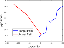
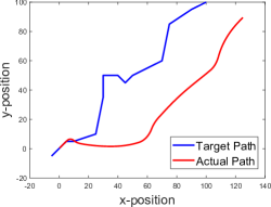
(a) With random intial weights	(b) At iteration 5
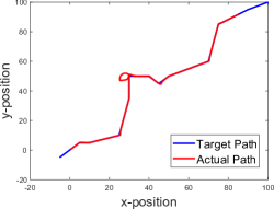
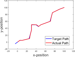
(c) At iteration 25	(d) At the end of the training

Figure 4: Evolution of the NN controller during the policy search.

The final parameter values arrived at by the CMA-ES algorithm are used as fixed weights and biases for the NN controller. Note that, after the training phase was completed, we validated the performance of the controller informally by observing behaviors for a set of random reference trajectories, and we observed reasonable performance from the system.

4.3 Verification Results

We applied the approach described in Section 3 to our case study, for a number of different versions of the NN controller described above. Each version of the system we consider contains a different number of neurons in the hidden layer. By evaluating our technique on this suite of systems, we demonstrate how well the method scales with the size of the NN.

For our evaluations, we assume that the target path for the controller is a straight line. For each verification, $X_{0}$ is given by the rectangular area defined by the diagonal corners $(-1.0,-\pi/16)$ and $(1.0,\pi/16)$, and $U$ is the complement (outside) of the rectangle described by the diagonal corners $(-5.0,-(pi/2-\epsilon))$ and $(5.0,(pi/2-\epsilon))$. The domain of interest for the barrier search is defined as $\mathcal{D}=(X_{0}\cup U)^{\prime}$, where $S^{\prime}$ is the complement of set $S$.

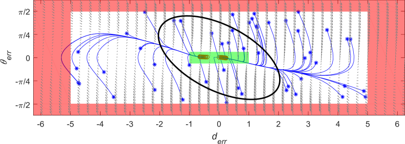
Figure 5: Phase portrait with sample system trajectories, $X_{0}$, $U$ and a barrier certificate level set.

Table 1 presents the experimental results. Each row of the table reports the time taken and number of iterations for each step of the procedure described in Fig. 1 applied to different versions of the system shown in Fig. 2 (where the versions differ in the complexity of the neural network-based controller used). The numbers shown correspond to average values over $30$ experiments; each experiment uses a unique seed to generate the initial simulations used to produce $\Phi_{s}$ in Fig. 1. The first column of the table indicates how many neurons are present in the hidden layer of the NN. The second column indicates the time spent to find a generator function (i.e., the time taken to complete the iterations of the first loop in Fig. 1). The third column indicates the average number of iterations needed to find a generator function. Each iteration consists of Solve LP and SMT Solver Check (5) operations as shown in Fig. 1. The third and fourth columns indicate the average time spent in each execution of Solve LP and SMT Solver Check (5) operations, respectively. The fifth column indicates the total amount of time spent in the operations given in Fig. 1 and not captured in the previous columns. The last column indicates the total time. Experimental results show that our approach scales well with the increasing number of neurons in the controller. We note that dReal uses heuristics to perform branch and prune operations, and although our experimental results show that it is generally able to solve long queries quickly, in the worst-case, SMT solutions can be costly. This occasional poor performance is exemplified in some of our experiments (e.g., the 300 and 500 neuron cases). We refer the reader to [7, 8] for a more detailed computational complexity analysis for dReal.

Number	Computing Generator					Time Spent	Total
of	Avg. Num.	Time Spent (s.)				in Other	Time
Neurons	Iterations	LP	Query	Total		Steps (s.)	(s.)
10	3.0	1.1	4.25	43		12	55
20	1.8	1.1	2.6	21		11	32
40	1.7	1.2	5.3	26		14	40
50	1.5	1.6	4.8	35		14	49
70	2.8	1.8	15.6	106		16	122
80	1.2	1.7	4.3	28		15	43
90	1.0	2.0	4.7	27		16	43
100	1.7	1.1	4.1	21		14	35
300	1.7	1.8	379.8	698		48	746
500	1.3	1.9	379.4	536		107	643
700	1.0	2.0	19.1	41		35	76
1000	1.0	2.0	50.4	74		79	153

Table 1: Timing analysis on safety verification for various versions of the system illustrated in Fig. 2.

Figure 5 illustrates the results of verification for one of the cases captured in Table 1. The lateral axis of the figure represents the position error (i.e., the $d_{err}$ state), and the vertical axis represents the angle error ($\theta_{err}$). The initial condition set $X_{0}$ is shown in green, and the unsafe set $U$ is shown in red. The simulation trajectories $\Phi_{s}$ are shown in blue; initial conditions for each trajectory are marked with an ($\ast$) and end points are marked with a ($\circ$). The sample space for the initial states is the $\mathcal{D}$ region. The ellipsoid between the $X_{0}$ and $U$ sets in Figure 5 is a level set of a generator function found using our approach; the barrier properties (5), (6), and (7) are all determined to be UNSAT by the dReal SMT solver [8]. Hence, the ellipsoid is a barrier certificate for the system, which means that the system is safe.

5 Conclusion

In this paper, we present a technique to reason about safety of a closed-loop control system using a learning-enabled controller. In particular, we focus on feedforward artificial neural network-based controllers. The key idea of our approach is to reduce the safety verification problem to the identification of a barrier certificate candidate, using simulations of the closed-loop system, and then perform a posteriori verification of the synthesized barrier certificate. The final verification step is performed using a nonlinear SMT solver, which permits our approach to handle neural networks with arbitrary nonlinear activation functions. We demonstrate the feasibility of our technique on a simple closed-loop model of a path-following ground vehicle. Future work will focus on improving the scalability of our technique and investigating stateful controllers based on recurrent neural networks. We will also investigate algorithms to simultaneously train the neural network while satisfying safety guarantees.

References

- [1]
- [2] Ayca Balkan, Jyotirmoy V Deshmukh, James Kapinski & Paulo Tabuada (2015): Simulation-guided Contraction Analysis. In: Proc. of the 1st Indian Control Conference, pp. 71–75.
- [3] Ayca Balkan, Paulo Tabuada, Jyotirmoy V Deshmukh, Xiaoqing Jin & James Kapinski (2018): Underminer: A Framework for Automatically Identifying Nonconverging Behaviors in Black-Box System Models. ACM Transactions on Embedded Computing Systems (TECS) 17(1), p. 20.
- [4] Tommaso Dreossi, Alexandre Donzé & Sanjit A Seshia (2017): Compositional falsification of cyber-physical systems with machine learning components. In: NASA Formal Methods Symposium, Springer, pp. 357–372.
- [5] Souradeep Dutta, Susmit Jha, Sriram Sanakaranarayanan & Ashish Tiwari (2017): Output Range Analysis for Deep Neural Networks. arXiv preprint arXiv:1709.09130.
- [6] Ruediger Ehlers (2017): Formal verification of piece-wise linear feed-forward neural networks. In: International Symposium on Automated Technology for Verification and Analysis, Springer, pp. 269–286.
- [7] Sicun Gao, Jeremy Avigad & Edmund Clarke (2012): Delta-Complete Decision Procedures for Satisfiability over the Reals. In: Logic in Computer Science.
- [8] Sicun Gao, Soonho Kong & Edmund M Clarke (2013): dReal: An SMT solver for nonlinear theories over the reals. In: International Conference on Automated Deduction, Springer, pp. 208–214.
- [9] Nikolaus Hansen & Andreas Ostermeier (2001): Completely derandomized self-adaptation in evolution strategies. Evolutionary computation 9(2), pp. 159–195.
- [10] Xiaowei Huang, Marta Kwiatkowska, Sen Wang & Min Wu (2017): Safety verification of deep neural networks. In: International Conference on Computer Aided Verification, Springer, pp. 3–29.
- [11] Christian Igel (2003): Neuroevolution for reinforcement learning using evolution strategies. In: Evolutionary Computation, 2003. CEC’03. The 2003 Congress on, 4, IEEE, pp. 2588–2595.
- [12] James Kapinski, Jyotirmoy V. Deshmukh, Sriram Sankaranarayanan & Nikos Aréchiga (2014): Simulation-guided Lyapunov Analysis for Hybrid Dynamical Systems. In: Hybrid Systems: Computation and Control.
- [13] Guy Katz, Clark Barrett, David L Dill, Kyle Julian & Mykel J Kochenderfer (2017): Reluplex: An efficient SMT solver for verifying deep neural networks. In: International Conference on Computer Aided Verification, Springer, pp. 97–117.
- [14] Stephen Prajna (2005): Optimization-based methods for nonlinear and hybrid systems verification. Ph.D. thesis, California Institute of Technology, Caltech, Pasadena, CA, USA.
- [15] Stephen Prajna & Ali Jadbabaie (2004): Safety Verification of Hybrid Systems Using Barrier Certificates. In: In Hybrid Systems: Computation and Control, Springer, pp. 477–492.