Motor Unit Number Estimation via Sequential Monte Carlo

Abstract

A change in the number of motor units that operate a particular muscle is an important indicator for the progress of a neuromuscular disease and the efficacy of a therapy. Inference for realistic statistical models of the typical data produced when testing muscle function is difficult, and estimating the number of motor units from these data is an ongoing statistical challenge. We consider a set of models for the data, each with a different number of working motor units, and present a novel method for Bayesian inference, based on sequential Monte Carlo, which provides estimates of the marginal likelihood and, hence, a posterior probability for each model. To implement this approach in practice we require sequential Monte Carlo methods that have excellent computational and Monte Carlo properties. We achieve this by leveraging the conditional independence structure in the model, where given knowledge of which motor units fired as a result of a particular stimulus, parameters that specify the size of each unit’s response are independent of the parameters defining the probability that a unit will respond at all. The scalability of our methodology relies on the natural conjugacy structure that we create for the former and an enforced, approximate conjugate structure for the latter. A simulation study demonstrates the accuracy of our method, and inferences are consistent across two different datasets arising from the same rat tibial muscle.

Keywords

Motor Unit Number Estimation; Sequential Monte Carlo; Model Selection

1 Introduction

Motor unit number estimation (MUNE) is a continuing challenge for clinical neurologists. An ability to determine the number of motor units (MUs) that operate a particular muscle provides important insights into the progression of various neuromuscular ailments such as amyotrophic lateral sclerosis (Shefner et al., 2006; Bromberg, 2007), and aids the assessment of the efficacy of potential therapy treatments (Casella et al., 2010).

A MU is the fundamental component of the neuromuscular system and consists of a single motor neuron and the muscle fibres whos contraction it governs. Restriction to a MU’s operation may be a result of impaired communication between the motor neuron and muscle fibres, abnormaility in their function, or atrophy of either cell type. A direct investigation into the number of MUs via a biopsy, for example, is not helpful since this only determines the presence of each MU, not its functionality.

Electromyography (EMG) provides a set of electrical stimulii of varying intensity to a group of motor neurons; each stimulus artificially induces a twitch in the targeted muscle, providing an in situ measurement of the functioning of the MUs. The effect on the muscle may be measured by recording either the minute variation in muscle membrane potential or the physical force the muscle exerts (Major and Jones, 2005). The generic methods developed in this article are applicable to either type of measurement. Since our data consist of whole muscle twitch force (WMTF) measurements we henceforth describe the response in these terms. In a healthy subject, the stimulus-response curve is typically sigmoidal (Henderson et al., 2006), illustrating the smooth recruitment of additional MUs as the stimulus increases; however, the relatively low number of MUs in a patient with impaired muscle function may manifest within the stimulus-response relationship as large jumps in WMTF measurements.

Figure 1 shows the two data sets that will be described and analysed in detail in Section 5, with the large jumps clearly visible. The histograms of absolute differences in response for adjacent stimuli show two main modes, one, near 0 mN, corresponding to noise and the other, around 40 mN indicating that different MUs fired. The noise arises primarily because of small variations in the contribution to the WMTF provided by any particular MU, whenever it fires. The second general source of noise, visible in isolation at very low stimuli when no MUs are firing, is called the baseline noise. This arises from respiration movements and pulse pressure waves, and particular care is taken to minimise such influences, for example by earthing the subject and equipment, restraining the limb, digitally resetting the force signal prior to each stimulus, synchronising stimuli with the pulse cycle and using highly sensitive measurement devices.

MUNE uses the observed stimulus-response pattern to estimate the number of functioning MUs. Techniques for MUNE generally form two classes: the average and comprehensive approaches. The most common averaging approach is the incremental technique of McComas et al. (1971), which assumes that the MUs can be characterised by an ‘average’ MU with a particular single motor unit twitch force (MUTF), estimated as the average of the magnitudes of the observed stepped increases in twitch force. A large stimulus, known as the supramaximal stimulus, is applied in order to cause all MUs to react. The quotient of the WMTF arising from the supramaximal stimulus and the average MUTF provides a count estimate. However, there is no guarantee that a particular single-stepped increase in response corresponds to a new, previously latent, MU, since it may instead be due to a phenomenon called alternation (Brown and Milner-Brown, 1976). This occurs when two or more MUs have similar activation thresholds such that different combinations of MUs may fire in reaction to two identical stimuli. Consequently, the incremental technique tends to underestimate the average MUTF and hence overestimate the number of MUs. A number of improvements both experimentally (Kadrie et al., 1976; Stashuk et al., 1994, e.g.) and empirically (Daube, 1995; Major et al., 2007, e.g.) have been proposed to try to deal with the alternation problem but, despite these improvements, each method oversimplifies the data generating mechanism and there is no gold-standard averaging approach; Bromberg (2007) and Gooch et al. (2014) provide thorough discussions on these approaches to MUNE.

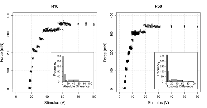
Figure 1: Stimulus-response curve from a rat tibial muscle using 10 µsec (left) and 50 µsec duration stimuli. Histogram inserts represent the frequency in the absolute difference of twitch forces when ordered by stimulus.

Motor units are more diverse than simple replicates of the ‘average’ MU, with many factors influencing their function. A desire for a more complete model for the data generating mechanism motivated the comprehensive approach to MUNE in Ridall et al. (2006), which proposed three assumptions:

• MUs fire independently of each other and of previous stimuli in an all-or-nothing response. Each MU fires precisely when the stimulus intensity exceeds a random threshold whose distribution is unique to that MU, with a sigmoidal cumulative distribution function, called an excitability curve.

• The firing of a MU is characterised by a MUTF which is independent of the size of the stimulus that caused it to fire, and has a Gaussian distribution with an expectation specific to that MU and a variance common to all MUs.

• The measured WMTF is the superposition of the MUTFs of those MUs that fired, together with a baseline component which has a Gaussian distribution with its own mean and variance.

From these assumptions, Ridall et al. (2006) proposed a set of similar statistical models each of which assumed a different fixed number of MUs. MUNE thus reduced to selection of a best model, for which the Bayesian information criterion was used. The class of methods which performs MUNE within a Bayesian framework is commonly referred to as Bayesian MUNE. In a subsequent paper, Ridall et al. (2007) extended the method by constructing a reversible jump Markov chain Monte Carlo (RJMCMC) (Green, 1995) to sample from the MU-number posterior mass function directly. However, its implementation is highly challenging with slow and uncertain convergence particularly when the studied muscle has many MUs. This is partly attributed to difficulty in defining efficient and meaningful transitions between models, with transition rates found to be 0.5–2% (Andrieu, 2007). The between model transition rate was improved in Drovandi et al. (2014) where it was noticed that under Assumption A1, for a given stimulus, the majority of MUs are either almost certain to fire or almost certain to not fire. Approximating this near certainty by absolute certainty led to a substantial reduction in the size of the sample space. The approximate sample space for the firing events was sufficiently small to permit marginalisation in the calculation of between-model transition probabilities, increasing the acceptance rate to 9.2% with simulated examples. Nevertheless, substantial issues over convergence remain as the parameter posterior distributions for models with more than the true number of MUs are multimodal.

In this paper, slight alterations of the neuromuscular assumptions permit the development of a fully adapted sequential Monte Carlo (SMC) filter, leading to SMC-MUNE, the first Bayesian MUNE method compatible with real-time analysis. As in Ridall et al. (2006), the principal inference targets are separate estimates of the marginal likelihood for models with $u=1,\ldots,u_{\max}$ MUs, for some maximum size $u_{\max}$.

The paper proceeds as follows. Section 2 presents the neuromuscular model of Ridall et al. (2006) for a fixed number of MUs and defines the priors for the model parameters. Section 3 describes the SMC-MUNE method. Due the complexity of the problem that MUNE addresses, this section is broken into three parts: inference for the firing events and associated parameters; inference for the parameters of the baseline and MUTF processes; and, estimation of the marginal likelihood so as to evaluate the posterior mass function for MU-number. Section 4 assesses the performance of the SMC-MUNE method for $200$ simulated data sets. Closer examination of cases where the point estimate of the number of MUs was incorrect revealed two classes of error; an example in each of these classes is investigated in detail. Section 5 applies the SMC-MUNE method to data (collected using the method in (Casella et al., 2010)) from a rat tibial muscle that has undergone stem cell therapy. Section 6 concludes the paper with a discussion on the effectiveness of SMC-MUNE and of potential avenues for improvement.

2 The neuromuscular model and prior specification

The three assumptions A1–A3 underpin a comprehensive description of the neuromuscular system. This section expands on these assumptions to form the model of the neuromuscular system for a given fixed number of MUs. Section 2.1 introduces the notational convention. Section 2.2 presents the neuromuscular model under the assumptions of Ridall et al. (2006), and Section 2.3 defines the prior distributions for the model parameters.

2.1 Notation

The total number of MUs operating the muscle of interest is denoted by $u$ and a particular MU is indexed by $j$. An EMG data set consists of $T$ measurements whereby the datum for the $t$th test, $t=1,\ldots,T$, consists of the applied stimulus $s_{t}$ and resulting WMTF $y_{t}$. The data set is re-ordered such that the observation $y_{1},\ldots,y_{\tau-1}$ define baseline measurements with $s_{t}=0$ for $t=1,\ldots,\tau-1$, followed by an overall WMTF $y_{\tau}$ corresponding to the supramaximal stimulus $s_{\tau}=\max_{t}(s_{t})$ where all $u$ MUs are known (by the clinician) to have fired. The remaining measurements appear in order of increasing stimulus. The advantages of this ordering will become evident in Section 3.3.

The reaction of MU $j$ to stimulus $s_{t}$ is denoted by the indicator variable $x_{j,t}$, which is $1$ if MU $j$ fires, and hence contributes to the $y_{t}$ measurement, and $0$ otherwise. The $u$-vector of indicators $\mathbf{x}_{t}=(x_{1,t},\ldots,x_{u,t})^{\top}$ defines the firing vector of the MUs in response to stimulus $s_{t}$. Given the experimental set-up, it is assumed that no MUs fire for any baseline measurement, $x_{j,t}=0$ for each $j=1,\ldots,u$ and $t=1,\dots\tau-1$, and all MUs fire in response to the supramaximal stimulus, $x_{j,\tau}=1$.

A sequentially indexed set of elements, vectors or scalars shall be represented as $a_{1:t}:=\{a_{1},\ldots,a_{t}\}$. The vectors where all elements are zero or all are unity are denoted by $\mathbf{0}$ an $\mathbf{1}$ respectively. The indicator function $\mathbb{I}_{A}(x)$ is $1$ if $x\in A$ and $0$ otherwise.

2.2 The neuromuscular model

Following the assumptions A1–A3 of Ridall et al. (2006), the state-space neuromuscular model for the WMTF observations based on a fixed $u$ number of MUs is as follows.

$$X_{j,t}|s_{t},\eta_{j},\lambda_{j} \sim\mathrm{Bern}\left[F\left(s_{t};\eta_{j},\lambda_{j}\right)\right],$$ (1)

$$Y_{j,t}|\mathbf{X}_{t}=\mathbf{x}_{t},\bar{\mu},\bar{\nu},\boldsymbol{\mu},\nu \sim\mathrm{N}\left(\bar{\mu}+\mathbf{x}_{t}^{\top}\boldsymbol{\mu},\bar{\nu}^{-1}+\nu^{-1}\mathbf{x}_{t}^{\top}\mathbf{1}\right).$$ (2)

The WMTF in (2) is the sum of independent Gaussian contributions, firstly, from a baseline effect of $N(\bar{\mu},\bar{\nu}^{-1})$ and, secondly, from each MU that fires. If the $j$th MU fires then it makes a $N(\mu_{j},\nu^{-1})$ contribution to the WMTF. The parameters $\boldsymbol{\mu}=(\mu_{1},\ldots,\mu_{u})^{\top}$, $\nu$, $\bar{\mu}$, $\bar{\nu}$ are collectively referred to as the observation parameters. Each firing event in (1), $X_{j,t}$, is a Bernoulli random variable with success probability given by a sigmoidal function $F$ of the stimulus, called the excitability curve (Brown and Milner-Brown, 1976). The excitability parameters for the $t$th MU, $\eta_{j}$ and $\lambda_{j}$, characterise its excitation features; conditional on these values, firing events are independent. The acyclic graph in Figure 2 depicts the dependencies within the neuromuscular model. Key to the strategy in this paper is that the observational and excitability parameters are conditionally independent given the unobserved firing events $\mathbf{x}_{1:T}$.

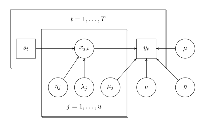
Figure 2: Directed acyclic graph of the neuromuscular model for a fixed number of motor units, $u$. Arrows denote direct dependencies between known data (square nodes) and unknown parameters and states (circle nodes). Pallets indicate repeated cases according to the stated index.

The excitability curve is a non-decreasing sigmoid function of the stimulus, parameterised by its median, $\eta$ and the reciprocal gradient at the median: $F(s=\eta;\eta,\lambda)=1/2$, and $F^{\prime}(s=\eta;\eta,\lambda)=1/\lambda$. Under assumption A1, Ridall et al. (2006) specifies the excitability curve as the Gaussian cumulative distribution function (CDF): $F(s)=\Phi[\delta(s-\eta)]$ where $\Phi(x)$ denotes the standard Gaussian CDF with $\delta=\sqrt{2\pi}/\lambda$. Evidence for this definition (Hales et al., 2004) focused on the central structure of the excitability curve by applying a binned chi-squared goodness-of-fit test. However, evidence to distinguish between this and alternatives such as the logistic curve will arise, chiefly, from tail events. Moreover, the Gaussian assumption allows a small, albeit potentially negligible, probability of a spurious firing event when no stimulus is applied. Given this contradiction with the experimental design, the following log-logistic form of the excitability is used:

$$F(s;\eta,\lambda)=\left[1+\left(\frac{s}{\eta}\right)^{-4\eta/\lambda}\right]^{-1}.$$ (3)

Nonetheless, the inference method described in Section 3.2 is applicable for any sigmoidal curve.

2.3 Prior distributions

The excitability parameters of individual MUs are assumed to be independent a priori. For some upper limits $\eta_{\max}$ and $\lambda_{\max}$, the excitability parameters are assigned vague independent beta prior distributions:

$$\frac{\eta}{\eta_{\max}}\sim\mathrm{Beta}(1.1,~{}1.1),\quad\quad\frac{\lambda}{\lambda_{\max}}\sim\mathrm{Beta}(1.1,~{}1.1).$$ (4)

The shape parameters are chosen so that the densities are uninformative yet tail off towards the boundaries. The location upper bound is conservatively set just greater than the supramaximal stimulus, $\eta_{\max}=1.1s_{\tau}$. Evidence for specifying the upper bound $\lambda_{\max}$ is taken from Hales et al. (2004) where, for a Gaussian excitability curve, the coefficient of variation of a random variable whose cumulative distribution function is given by the excitability curve was estimated to be 1.65%. With the log-logistic curve this corresponds to $\lambda/\eta\approx 3.64\%$. Given that $\eta\leq\eta_{max}=1.1s_{\tau}$, we deduce that $\lambda\leq 0.04s_{\tau}$. The limitations of the the study of Hales et al. (2004), commented on by Major et al. (2007), indicate that a larger bound may be required than initially suggested, so sensitivity of MUNE to $\lambda_{\max}$ is investigated in Sections 4.2 and 5.

The following pair of four-parameter (multivariate) Gaussian-gamma prior distributions are specified for the observation parameters:

$$\bar{\nu} \sim\mathrm{Gam}\left(\bar{a}_{0},~{}\bar{b}_{0}\right),\quad\quad\bar{\mu}|\bar{\nu}\sim\mathrm{N}\left(\bar{m}_{0},~{}\bar{\nu}^{-1}\bar{c}_{0}\right),$$

$$\nu \sim\mathrm{Gam}\left(a_{0},~{}b_{0}\right),\quad\quad\boldsymbol{\mu}|\nu\sim\mathrm{MVN}_{u}\left(\mathbf{m}_{0},~{}\nu^{-1}C_{0}\right).$$ (5)

All hyper-parameters are strictly positive scalars except for the real-valued scalar expectation $\bar{\mu}_{0}$, $u$-vector $\mathbf{m}_{0}$ and $u\times u$ positive definite matrix $C_{0}$. The prior distributions defined for the precision parameters are consistent with Ridall et al. (2006). However, the prior for both baseline and MUTF expectations differ from the gamma definition of Ridall et al. (2006). The tractability reasons for adopting Gaussian rather than gamma priors are detailed in Section 3.3; the problems that arise from the support now including the whole real line are addressed in Section 3.4.

The range of MUs to consider, $u=1,\ldots,u_{\max}$, defines a set of neuromuscular models. Previous Bayesian MUNE methods defined a uniform prior on the model space in assuming that each is equally probable. However, there is typically a preference for identifying the simplest representation of the underlying process. This is of particular importance in the presence of alternation where the data could be equally probably under two or more models. To impose an a priori preference for smaller models the number of MUs is given a $\mathsf{Geom}(1/2)$ distribution, truncated at $u_{\max}$.

3 Methodology for SMC-MUNE

The methodology that defines the SMC-MUNE procedure detailed in this section is based on an approximation to the ideal model defined in Section 2 using, effectively, an approximation to the prior specification. The reasons for the approximations are twofold: firstly, the choice of prior is necessary for certain tractable operations but does not reflect true prior belief; secondly, prior specification does not lead conveniently and efficiently to sequential inference yet a simple approximation achieves this goal. An overview of the methodology is first provided, with details about each part given subsequently. Adapting terminology from sequential inference, the re-ordered index $t$ shall henceforth be referred to as ‘time’.

3.1 Overview

The ultimate aim is to calculate and compare the posterior model probabilities for a range of models, each with a different number of MUs, $u$. Posterior model probabilities are straightforward to obtain once the marginal likelihood for each model is available. Hence, for a given model with $u$ MUs, the target for inference is its marginal likelihood, $f(y_{1:T}|s_{1:T})$; throughout this section, for notational simplicity, we suppress the dependence on $u$. This can be expressed as a product of sequential predictive factors with each defined by:

$$f\left(y_{t}|~{}y_{1:t-1},~{}s_{1:t}\right) =\sum_{\mathbf{x}_{1:t-1}\in\mathcal{X}_{1:t-1}}f\left(y_{t}|~{}\mathbf{x}_{1:t-1},~{}y_{1:t-1},~{}s_{1:t}\right)\mathbb{P}\left(\mathbf{x}_{1:t-1}|~{}y_{1:t-1},~{}s_{1:t-1}\right)$$ (6)

where $\mathcal{X}_{1:t}=\{0,1\}^{ut}$ denotes the space for the sequence of vectors of historical firing events.

The inference scheme is based upon two key observations. Firstly, the observation and excitability parameters are conditionally independent given the set of firing events $\mathbf{x}_{1:T}$. Such an independence structure separates the observational and firing processes and simplifies the marginalisation of the parameter space for evaluating the marginal likelihood. Secondly, conditional on $\mathbf{x}_{t}$, the priors for the observation parameters in (5) are nearly conjugate for the likelihood in (2). For a baseline measurement (which has $\mathbf{x}_{t}=\mathbf{0}$) the posterior has the same form as the prior with tractable updates; the same would be true for a non-baseline measurement ($\mathbf{x}_{t}\neq\mathbf{0}$) if it were possible to set $\bar{\nu}^{-1}=0$ and to ignore the further information on $\bar{\mathcal{A}}$; such an approximation is described and justified in Section 3.3.

Subject to this approximation, the posterior distribution for the observational parameters after assimilating $y_{1:t}$ and conditional on $\mathbf{x}_{1:t}$ is defined by the sufficient statistics and (multivariate) Gaussian-gamma distributions analogous to the prior specification:

$$\bar{\mathcal{A}}_{t}:=\left\{\bar{a}_{t},~{}\bar{b}_{t},~{}\bar{m}_{t},~{}\bar{c}_{t}\right\}\quad\mathrm{and}\quad\mathcal{A}_{t}:=\left\{a_{t},~{}b_{t},~{}\mathbf{m}_{t},~{}C_{t}\right\},$$ (7)

$$\bar{\nu}|y_{1:t},\mathbf{x}_{1:t} \sim\mathrm{Gam}\left(\bar{a}_{t},~{}\bar{b}_{t}\right),\quad\quad\bar{\mu}|\bar{\nu},y_{1:t},\mathbf{x}_{1:t}\sim\mathrm{N}\left(\bar{m}_{t},~{}\bar{\nu}^{-1}\bar{c}_{t}\right),$$

$$\nu|y_{1:t},\mathbf{x}_{1:t} \sim\mathrm{Gam}\left(a_{t},~{}b_{t}\right),\quad\quad\boldsymbol{\mu}|\nu,y_{1:t},\mathbf{x}_{1:t}\sim\mathrm{MVN}_{u}\left(\mathbf{m}_{t},~{}\nu^{-1}C_{t}\right).$$ (8)

Given the assumptions leading to (8) the marginal likelihood for the observation $y_{t}$ conditional on the firing vector $\mathbf{x}_{t}$ and sets $\bar{\mathcal{A}}_{t-1}$ and $\mathcal{A}_{t-1}$ has tractable form:

$$f\left(y_{t}|\mathbf{x}_{t},\bar{\mathcal{A}}_{t-1},\mathcal{A}_{t-1}\right) =\left\{\begin{array}[]{ll}\mathsf{t}\left[y_{t};~{}\bar{m}_{t-1},~{}\frac{\bar{b}_{t-1}}{\bar{a}_{t-1}}\left(\bar{c}_{t-1}+1\right),~{}2\bar{a}_{t-1}\right]&\mathrm{if}~{}\mathbf{x}_{t}=\mathbf{0},\\ \mathsf{t}\left[y_{t};~{}\bar{m}_{t-1}+\mathbf{x}_{t}^{\top}\mathbf{m}_{t-1},~{}\frac{b_{t-1}}{a_{t-1}}\left(\mathbf{x}_{t}^{\top}C_{t-1}\mathbf{x}_{t}+\mathbf{x}_{t}^{\top}\mathbf{1}\right),~{}2a_{t-1}\right]&\mathrm{otherwise}.\\ \end{array}\right.$$ (11)

Here, $\mathsf{t}(y;m,v,n)$ denotes the Student’s t-density function on $n$ degrees of freedom with centrality parameter $m$ and scaling factor $\sqrt{v}$. The statistics $\bar{\mathcal{A}}_{t-1}$ and $\mathcal{A}_{t-1}$ are deterministic functions of $y_{1:t-1}$ and $\mathbf{x}_{1:t-1}$, and are sufficient in that $f(y_{t}|\mathbf{x}_{1:t},y_{1:t-1})\equiv f(y_{t}|\mathbf{x}_{t},\bar{\mathcal{A}}_{t-1},\mathcal{A}_{t-1})$.

The posterior-predictive mass function for the next excitation vector, $\mathbb{P}\left(\mathbf{x}_{t}|\mathbf{x}_{1:t-1},y_{1:t-1},s_{1:t}\right)$
$=\mathbb{P}\left(\mathbf{x}_{t}|\mathbf{x}_{1:t-1},s_{1:t}\right)$, is given by the following intractable marginalisation:

$$\mathbb{P}\left(\mathbf{x}_{t}|\mathbf{x}_{1:t-1},s_{1:t}\right)=\int\mathbb{P}\left(\mathbf{x}_{t}|\eta_{1:u},\lambda_{1:u},s_{t}\right)\pi\left(\eta_{1:u},\lambda_{1:u}|\mathbf{x}_{1:t-1},s_{1:t-1}\right)~{}d\eta_{1:u}~{}d\lambda_{1:u},$$ (12)

where $\pi\left(\eta_{1:u},\lambda_{1:u}|\mathbf{x}_{1:t-1},s_{1:t-1}\right)$ is the posterior for the excitability parameters given the firing vectors to time $t-1$. Section 3.2 presents a fast numerical quadrature scheme for evaluating (12) to any desired accuracy.

The marginalisations over the parameters in (11) and (12) together provide the predictive:

$$f\left(y_{t}|~{}\mathbf{x}_{1:t-1},~{}y_{1:t-1},~{}s_{1:t}\right) =\sum_{\mathbf{x}_{t}\in\mathcal{X}_{t}}f\left(y_{t}|~{}\mathbf{x}_{1:t},~{}y_{1:t-1},~{}s_{1:t}\right)\mathbb{P}\left(\mathbf{x}_{t}|~{}\mathbf{x}_{1:t-1},~{}s_{1:t}\right),$$ (13)

Combination of (13) with the historical firing event mass function $\mathbb{P}\left(\mathbf{x}_{1:t}|y_{1:t},s_{1:t}\right)$ would provide the quantity $f(y_{t}|y_{1:t-1},~{}s_{1:t})$ in (6) as required; however, it is infeasible to track $\mathbb{P}\left(\mathbf{x}_{1:t}|y_{1:t},s_{1:t}\right)$ as the dimension of the event space increases exponentially with time. Instead, combining (11), (12) and (13) gives the conditional mass function for the current firing vector given all previous firing vectors and all MUTFs to date,

$$\mathbb{P}\left(\mathbf{x}_{t}|~{}y_{1:t},~{}\mathbf{x}_{1:t-1},~{}s_{1:t}\right) =\frac{f\left(y_{t}|~{}\mathbf{x}_{1:t},~{}y_{1:t-1},~{}s_{1:t}\right)\mathbb{P}\left(\mathbf{x}_{t}|~{}\mathbf{x}_{1:t-1},~{}s_{1:t}\right)}{f\left(y_{t}|~{}\mathbf{x}_{1:t-1},~{}y_{1:t-1},~{}s_{1:t}\right)}.$$ (14)

Expressions in (13) and (14) together lead to a fully adaptive sequential Monte Carlo (SMC) sampler which approximates the historical firing event mass function by the particle set $\left\{\mathbf{x}_{1:t}^{(i)}\right\}_{i=1}^{N}$, for a suitably large $N$, recursively updating the set for $t=1,\dots,T$. Algorithm 1 presents the auxiliary SMC sampler (Pitt and Shephard, 1999) which, given the set of samples drawn from $\mathbf{X}_{1:t-1}|~{}y_{1:t-1},~{}s_{1:t-1}$, creates an unweighted sample from the filtering distribution $\mathbf{X}_{1:t}|y_{1:t},s_{1:t}$, and approximates (6) via Monte Carlo so as to update the marginal likelihood estimate $\hat{f}(y_{1:t}|~{}s_{1:t})$.

Algorithm 1 Fully adapted SMC sampler

1:for $i$ in $1,\dots,N$ do $\triangleright$ Weight

2:     $\omega_{t}^{(i)}=f(y_{t}|\mathbf{x}_{1:t-1}^{(i)},~{}y_{1:t},~{}s_{1:t})$ $\triangleright$ Using (13)

3:$\bar{\omega}_{t}^{(i)}=\omega_{t}^{(i)}/\sum_{k}\omega_{t}^{(k)}$.

4:Sample auxiliary indices $\{\zeta^{(i)}\}_{i=1}^{N}$ with probabilities $\{\bar{\omega}_{t}^{(i)}\}_{i=1}^{N}$. $\triangleright$ Resample

5:for $i$ in $1,\dots,N$ do $\triangleright$ Propagate

6:     Sample $\mathbf{x}_{t}^{(i)}$ with probability $\mathbb{P}\left(\mathbf{x}_{t}|~{}y_{t},~{}\mathbf{x}_{1:t-1}^{(\zeta_{i})},~{}s_{1:t}\right)$. $\triangleright$ Using (14)

7:     Set $\mathbf{x}_{1:t}^{(i)}=\left(\mathbf{x}_{1:t-1}^{(\zeta_{i})},~{}\mathbf{x}_{t}^{(i)}\right)$.

8:Set $\log\hat{f}\left(y_{1:t}|~{}s_{1:t},~{}u\right)=\log\hat{f}\left(y_{1:t-1}|~{}s_{1:t-1},~{}u\right)-\log N+\log\sum_{i}\omega^{(i)}_{t}$. $\triangleright$ Update marginal likelihood

Although primary interest lies in the marginal-likelihood estimate, parameter inference is also available to assist in assessing the quality of fit. The deterministic map to the sufficient statistics from the set of firing events and responses permits the transformation from the final particle set $\{X_{1:T}^{(i)}\}_{i=1}^{N}$ to an $N$-component Gaussian-gamma mixture approximating the posterior distribution for the observation parameters. A similar transformation for evaluating the posterior distribution for the excitability parameters is derived from the approximation to the prior; see Section 3.2 for details.

3.1.1 Equivalent particle specification and degeneracy

The Bayesian conjugate structure for the observation process suggests storing and updating the sufficient statistics when assimilating the latest observations. Given the prior statistics $\bar{\mathcal{A}}_{0}$ and $\mathcal{A}_{0}$, there is a deterministic map from $(\mathbf{x}_{1:t-1},~{}y_{1:t-1})$ to $(\bar{\mathcal{A}}_{t-1},~{}\mathcal{A}_{t-1})$. Hence estimates relating to the observation process at time $t$ are equivalently expressed with respect to the samples $\{\bar{\mathcal{A}}_{t-1}^{(i)},~{}\mathcal{A}_{t-1}^{(i)},~{}\mathbf{x}_{t}^{(i)}\}_{i=1}^{N}$; the storage required for this set does not increase with with number of observations assimilated. Since the method relies on these sufficient statistics, Algorithm 1 may be considered as a case of particle learning (Carvalho et al., 2010). For notational clarity, however, the particle set is described in terms of the historical firing events, $\mathbf{x}_{1:t-1}$, unless otherwise specified.

Assimilating the observation, $y_{\tau}$, at the supramaximal stimulus, $s_{\tau}$, before any of the other non-baseline observations ensures an update for all MUs, $j$, from the initial vague priors for each $\mu_{j}$. After this, each $m_{j}\approx y_{\tau}/u$, ensuring more sensible predictions in (11) and hence (13), when a new MU fires. This helps to mitigate against the inevitable particle degeneracy that occurs with particle learning. Further mitigation is achieved by iteratively re-running the algorithm with more and more particles until inferences are stable (see Appendix A).

3.2 Details for the firing vector and excitability parameters

At time $t-1$, each particle sample consists of a historical sequence of firing events for all MUs, and from this an associated joint posterior for the firing parameters, $\eta_{1:u}$ and $\lambda_{1:u}$, is derived. A representation of the distribution for the excitability parameters is sought that is analogous to that described for the observation parameters in that it should (a) permit simple calculation of the firing event predictive (12), (b) be deterministically updatable when assimilating the current measurement, and (c) provide a concise and sufficient description for the posterior distribution.

From the independence of MU firing under Assumption A1 and the excitability parameter prior in (4), it follows that the predictive for the firing event $\mathbf{x}_{t}$ in (12) factorises:

$$\mathbb{P}\left(\mathbf{x}_{t}|~{}\mathbf{x}_{1:t-1},~{}s_{1:t}\right) =\prod_{j=1}^{u}\iint\mathbb{P}\left(x_{j,t}|~{}\eta_{j},~{}\lambda_{j},~{}s_{t}\right)\pi\left(\eta_{j},~{}\lambda_{j}|~{}x_{j,1:t-1},~{}s_{1:t-1}\right)d\eta_{j}~{}d\lambda_{j},$$ (15)

where the posterior at time $t-1$ for the excitability parameters associated with MU $j$ is:

$$\pi\left(\eta_{j},~{}\lambda_{j}|~{}x_{j,1:t-1},~{}s_{1:t-1}\right) \propto\prod_{r=1}^{t-1}\mathbb{P}\left(x_{j,r}|~{}\eta_{j},~{}\lambda_{j},~{}s_{r}\right)\pi\left(\eta_{j}\right)\pi\left(\lambda_{j}\right).$$ (16)

Regardless of the excitability curve definition, this product of firing probabilities does not lead to a simple conjugate structure with a concise set of sufficient statistics for the posterior distribution. Furthermore, whilst for specific values of $(\eta_{j},\lambda_{j})$ the update in (16) may be performed sequentially, the integrations for the normalising constant in (16) and the expectation in (15) require evaluation of the product at arbitrary values in a continuum. To address these issues, the following approximation is proposed:

• For each MU, store and update at each time point a surface proportional to the posterior density $\pi(\eta_{j},\lambda_{j}|x_{j,1:t-1},s_{1:t-1})$ at a set of grid of points on a regular rectangular lattice $\mathcal{G}$ spanning the excitability parameter space. For general $(\eta_{j},\lambda_{j})$, approximate the right-hand side of (16) using bilinear interpolation from the four nearest grid points.

Under this assumption, let $h(\eta,~{}\lambda)$ be the right-hand side of (16); then $\tilde{h}(\eta,~{}\lambda)$, the interpolated surface specified using points on the unit square in which $(\eta,\lambda)$ resides, is:

$$\tilde{h}(\eta,\lambda) =(1-\eta)(1-\lambda)h(0,0)+(1-\eta)\lambda h(0,1)+\eta(1-\lambda)h(1,0)+\eta\lambda h(1,1),$$

with a similar approximation for $\mathbb{P}\left(x_{j,t}|\eta_{j},\lambda_{j},s_{t}\right)h(\eta_{j},\lambda_{j})$ based on interpolating this between grid points. The resulting approximations for the normalising constant in (16) and the integral in (15), therefore, correspond to iterative (over the two dimensions) application of the compound trapezium rule. This approach provides a deterministic updating procedure for maintaining the excitability posterior density up to a constant of proportionality for each point on the regular lattice.

A naïve implementation of the above scheme would evaluate the posterior density for each grid point, MU and particle sample. However, two posterior densities will only differ if the historical firing events differ. Consider any two particles, $i$ and $i^{\prime}$, each with an associated MU, $j$ and $j^{\prime}$ respectively, that have identical firing histories: $x_{j,1:t}^{(i)}=x_{j^{\prime},1:t}^{(i^{\prime})}$. Since the priors for the excitability parameters are identical for all MUs then the posterior distribution for these two MUs on these two particles are identical. Efficiency gains are therefore achieved by storing a single grid of values for each unique firing pattern to date.

A higher-order Newton-Cotes numerical integration method would produce a more accurate estimate of (15), but the associated interpolated density surface of piecewise polynomials would not be guaranteed to be bounded below by zero, making an inspection of parameter estimates for assessing model fit problematic. Alternatively, quadrature on adaptive sparse grids (Bungartz and Dirnstorfer, 2003), where the grid is finer at regions of high curvature, could improve estimator accuracy over the static regular rectangular lattice. However, this would be achieved at the expense of additional implementation complexity and further approximation error when estimating the surface at infilled lattice points.

3.3 Details concerning the observation process

Consider the observation model (2). At time $t\leq\tau-1$, when no MUs fire, $\mathbf{x}_{t}=\mathbf{0}$, the observation, $y_{t}$, provides no new information about the observation parameters for the MUs, $\mathcal{A}_{t}=\mathcal{A}_{t-1}$, and $Y_{j,t}|\mathbf{x}_{t}=0,\bar{\mu},\bar{\nu},\boldsymbol{\mu},\nu\sim\mathrm{N}(\bar{\mu},\bar{\nu}^{-1})$. Standard conjugate updates may, therefore, be applied to obtain $\bar{\mathcal{A}}_{t}$ as follows:

$$\bar{m}_{t}=\bar{m}_{t-1}+\frac{y_{t}-\bar{m}_{t-1}}{1+\bar{c}_{t-1}},\quad\bar{c}_{t}=\frac{\bar{c}_{t-1}}{1+\bar{c}_{t-1}},\quad\bar{a}_{t}=\bar{a}_{t-1}+\frac{1}{2},\quad\bar{b}_{t}=\bar{b}_{t}+\frac{(y_{t}-\bar{m}_{t-1})^{2}}{2(1+\bar{c}_{t-1})}.$$

When $t\geq\tau$, at least one MU fires and tractable updates are not possible. However, in real experiments, because of the precautions detailed in Section 1, the variance (and expectation) of the baseline noise are generally much smaller than the variability in response from a given MU when it fires. For example Henderson et al. (2006) find a ratio of an order of magnitude. We, therefore make the following approximation:

• When assimilating a non-baseline observation, $\bar{\mathcal{A}}$ is kept fixed at its previous value, and for updating $\mathcal{A}$ it is assumed that $\bar{\nu}^{-1}=0$.

Approximation B2 implies that for $\mathbf{x}_{t}\neq\mathbf{0}$,

$$Y_{t}|~{}\bar{\nu},~{}\boldsymbol{\mu},~{}\nu,~{}\bar{\mathcal{A}}_{t-1},~{}\mathcal{A}_{t-1} \stackrel{{\scriptstyle apx.}}{{\sim}}\mathrm{N}\left(~{}\bar{m}_{t-1}+\mathbf{x}_{t}^{\top}\boldsymbol{\mu},~{}\nu^{-1}\mathbf{x}_{t}^{\top}\mathbf{1}~{}\right),$$

which, given distributions at time $t-1$ as specified in (8), leads to the desired tractable updates for the sufficient statistics for (7) as follows: $\bar{\mathcal{A}}_{t}=\bar{\mathcal{A}}_{t-1}$ and

$$\mathbf{m}_{t} =\mathbf{m}_{t-1}+q_{t}C_{t-1}\mathbf{x}_{t}(y_{t}-\bar{m}_{t}-\mathbf{x}_{t}^{\top}\mathbf{m}_{t-1}) C_{t} =C_{t-1}-q_{t}C_{t-1}\mathbf{x}_{t}\mathbf{x}_{t}^{\top}C_{t-1}$$

$$a_{t} =a_{t-1}+\frac{1}{2} b_{t} =b_{t-1}+\frac{q_{t}}{2}(y_{t}-\bar{m}_{t}-\mathbf{x}_{t}^{\top}\mathbf{m}_{t-1})^{2},$$

where $q_{t}=(\mathbf{x}_{t}^{\top}\mathbf{1}+\mathbf{x}_{t}^{\top}C_{t-1}\mathbf{x}_{t})^{-1}$. In essence, the approximate observation process decouples the learning about the observational parameters: when no MU fires then $(\bar{\mu},\bar{\nu})$ is updated, else $(\mu,\nu)$ is updated.

After assimilating the baseline observations $y_{1},\dots,y_{\tau-1}$, both $\bar{\nu}^{-1}$ and $\bar{\mu}$ are known (and known to be small) with considerable certainty. Thus, approximating $\bar{\nu}^{-1}$ as $0$ and considering $\bar{\mu}$ to be a point mass at $\bar{m}$ is reasonable. Furthermore, the prior for $\nu$ does not need to be set until just before the observation $y_{\tau}$ is assimilated. Given the tight posterior for $\bar{\nu}$ at this juncture it is, therefore, possible to incorporate the knowledge that $\bar{\nu}>>\nu$ into the vague prior for $\nu$ (which is conceptually equivalent to specifying an initial joint prior on $\bar{\nu}$ and $\nu$). Letting $\bar{\nu}_{\tau-1}^{\mbox{\scriptsize med}}$ denote the posterior median of $\bar{\nu}$ at time $\tau-1$, tuning parameters $\epsilon<<1$ and $\delta<<1$ are chosen such that $\mathbb{P}(\nu>\epsilon\bar{\nu})\approx\delta$ is desired. Given that

$$1-\delta=\mathbb{P}(\nu\leq\epsilon\bar{\nu})\approx\mathbb{P}(\nu\leq\epsilon\bar{\nu}_{\tau-1}^{\mbox{\scriptsize med}})=\mbox{{Gam}}(b_{\tau-1}\epsilon\bar{\nu}_{\tau-1}^{\mbox{\scriptsize med}};~{}a_{\tau-1}),$$ (17)

where $\mbox{{Gam}}(x;\alpha)$ is the cumulative distribution function evaluated at $x$ of a gamma random variable with shape $\alpha$ and unit rate, a practical specification for the prior for $\nu$ is obtained by defining a small $a_{\tau-1}=a_{0}$ and then solving (17) for $b_{\tau-1}$.

3.4 Improving the marginal likelihood estimate

The following post-processing development is motivated by the analysis of a particular simulated dataset where the point estimate for the number of MUs is one greater than the true number. The detailed analysis in Section 4.1 shows that the extra MU has a very weak expected MUTF and that it, effectively, acts simply to increase the variability in the response. The problem arises because the $u$-vector, $\boldsymbol{\mu}$, of expected MUTF contributions has a Gaussian prior which, to allow reasonable uncertainty across the typical range of believable MUTF contributions, also places a non-negligible prior mass at low and even negative values. Negative expectations for an individual MU need not be prohibited by the data provided that MU is always inferred to fire alongside another MU with a positive expectation of similar or larger magnitude. The fact that the parameter suport permits this possibility potentially increases the marginal likelihood for a model which is larger than that necessary to explain the data.

Guaranteeing positive MUTFs greater than some minimum (Bromberg, 2003; Major et al., 2007) would require a change to the likelihood. The approach taken in Ridall et al. (2006) is to specify independent left-truncated gamma prior distributions for the the expected MUTFs, $\mu_{j}$ for $j=1,\ldots,u$. However any such change would not lead to the tractable updates required for the concise sequential analysis described in Sections 3.1 and 3.3. Within the constraints of the algorithm overviewed in Section 3.1, the natural mechanism for preventing these undesirable scenarios is via post-processing: the conditional prior for $\boldsymbol{\mu}|\nu$ in (5) is re-calibrated by truncating it to the region $M=[\mu_{\min},\infty)^{u}$ for some minimum MUTF $\mu_{\min}$. It follows that the re-calibrated marginal prior for $\boldsymbol{\mu}$ is:

$$\tilde{\pi}(\boldsymbol{\mu}) =\frac{1}{\pi(M)}\pi(\boldsymbol{\mu})\mathbb{I}_{M}(\boldsymbol{\mu}),$$ (18)

where $\pi(\boldsymbol{\mu})$ is the multivariate Student’s t-density centred at $\mathbf{m}_{0}$ with shape matrix $\frac{b_{0}}{a_{0}}C_{0}$ and $2a_{0}$ degrees of freedom, and, with a slight abuse of notation, $\pi(M)=\int_{M}\pi(\boldsymbol{\mu})d\boldsymbol{\mu}$. The effect on the marginal likelihood from the prior re-calibration is examined by Proposition 1.

Proposition 1.

Let $f(y_{1:T}|s_{1:T})$ denote the marginal likelihood defined in Section 3.1. The re-calibrated marginal likelihood, denoted by $\tilde{f}(y_{1:T}|s_{1:T})$, resulting from truncating the prior for $\boldsymbol{\mu}$ in (5) to $M$ is:

$$\tilde{f}(y_{1:T}|s_{1:T})=\frac{\pi(M|y_{1:T},s_{1:T})}{\pi(M)}f(y_{1:T}|s_{1:T})=\frac{\pi(M|y_{1:T},s_{1:T})}{\pi(M|y_{1:\tau-1},s_{1:\tau-1})}f(y_{1:T}|s_{1:T}),$$ (19)

where $\pi(M|y_{1:t},s_{1:t})=\int_{M}\pi(\boldsymbol{\mu}|y_{1:t},s_{1:t})d\boldsymbol{\mu}$.

Proof.

Expressing the re-calibrated marginal likelihood as a marginalisation of $\boldsymbol{\mu}$ and substituting the definition (18) produces the first equality by:

$$\tilde{f}(y_{1:T}|s_{1:T})=\int\tilde{\pi}(\boldsymbol{\mu})f(y_{1:T}|\boldsymbol{\mu},s_{1:T})d\boldsymbol{\mu}=\frac{\int_{M}\pi(\boldsymbol{\mu})f(y_{1:T}|\boldsymbol{\mu},s_{1:T})d\boldsymbol{\mu}}{\pi(M)}=\frac{\pi(M|y_{1:T},s_{1:T})}{\pi(M)}f(y_{1:T}|s_{1:T}).$$

The second equality in (19) arises as the first $\tau-1$ observations relate exclusively to the baseline.

Evaluation of $\pi(M|y_{1:\tau-1},s_{1:\tau-1})$ is straightforward since it is an orthant probability for the multivariate Student-t distribution. In contrast, the posterior probability is estimated from the $N$-component-mixture approximation of the posterior distribution by the final particle set:

$$\hat{\pi}(M|y_{1:T},s_{1:T}) =\frac{1}{N}\sum_{i=1}^{N}\pi(M|\mathbf{x}_{1:T}^{(i)},y_{1:T}).$$

∎

There is no theoretical argument against assuming (18) from the outset. Indeed, the firing events sampled in the propagation step of Algorithm 1 would then account for the restriction to the $\boldsymbol{\mu}$ parameter space and therefore directing particle samples to a more appropriate approximation for posterior parameter estimates. However, implementing this scheme requires at most $N2^{u}$ orthant evaluations of the multivariate Student’s t-distribution per time step in calculating the re-sampling weights. Standard procedures for evaluating these orthant probabilities (Genz and Bretz, 2009) are expensive, so the computational time of the resulting SMC-MUNE algorithm would increase substantially.

4 Simulation study

The performance of the SMC-MUNE algorithm is now assessed using $200$ simulated data sets, $20$ for each true number of MUs of $u^{*}=1,\ldots,10$. Each data set consists of $T=220$ measurements with $\tau=21$ so that the first $20$ observations correspond to the baseline, $s_{t}=0$ V, and these are followed by the supramaximal stimulus $s_{21}=40$ V.

All MUs are excited according to the log-logistic curve (3) with MU parameters simulated anew for each dataset as follows: $\eta_{j}\sim\mathsf{Unif}(5,40)$, $\lambda_{j}\sim\mathsf{Gamma}(2,8)\mathbb{I}(\lambda_{j}<10)$, $\mu_{j}\sim\mathsf{N}(40,20^{2})\mathbb{I}(\mu_{j}>20)$, $\nu^{-1}\sim\mathsf{Unif}(1,5)$. The measurement units for excitation parameters are all in V and the expected MUTFs are in mN with variance parameter in mN². Parameters were independent except for the following constraints, where $(j)$ is the index of the MU with the $j$th highest $\eta$ value: $\eta_{(j)}-\eta_{(j-1)}>2$ (neigbours must be separate) and $|\mu_{(j)}-\mu_{(j-1)}|>4$ (neighbours should have distinct expectations). To test the ability of SMC-MUNE, these values ensure a greater range in MUTF contributions and in the excitation parameters than is typically observed in practice. For example, the average coefficient of variation is $11.2\%$ (as opposed to $1.65\%$; see Section 2.3). This resulted in $79\%$ of datasets containing at least one alternation event. Additional noise was generated as in (2) with $\bar{\mu}=0$ mN and $\bar{\nu}^{-1}=0.25^{2}$ mN².

To each data set, a set of neuromuscular models was fitted with a number of MUs, $u$, ranging from $1$ up to a maximum size of $u_{\max}=12$. The sufficient statistics for the parameter prior distributions are provided in Appendix A. To control the Monte Carlo variability and the error in the numerical integration, the particle set size, $N$, and the lattice size for numerical integration were iteratively increased until estimates of the marginal likelihood were stable; see Appendix A for further details. The point estimate of the number of MUs is taken to be the maximum a posteriori (MAP) model, $\hat{u}$, and uncertainty in the estimate is quantified by the 95% highest posterior credible set (HPCS); the minimal set of models where their total posterior probability is at least 95%. In addition, the estimated posterior probability for the true model, $p_{u^{*}}=\hat{\mathbb{P}}(U=u^{*}|y_{1:T},s_{1:T})$, is evaluated.

Table 1: Summary of the MU-number posterior mass functions and required numerical resource for 200 simulated data sets.

Number of MUs, $u^{*}$	$\leq 5$	6	7	8	9	10
No. where $\hat{u}=u^{*}$	100	19	19	16	15	12
No. where $u^{*}$ in HPCS	100	20	20	19	19	20
Avg. size of HPCS	1.11	1.70	2.10	2.05	2.35	2.45
Avg. $\hat{p}_{u^{*}}$ (%)	97.95	89.20	80.45	69.42	62.70	54.68
Avg. particle set size for $u^{*}$	5000	5250	6000	7500	7500	8250
Avg. particle set size for $\hat{u}$	5000	5000	6000	7500	9250	7750
Avg. $n{\times}n$ lattice size for $u^{*}$	30.0	30.5	30.5	32.0	32.5	32.0
Avg. $n{\times}n$ lattice size for $\hat{u}$	30.0	30.0	30.5	32.0	35.0	32.0

Table 1 presents summaries of the mass functions of the number of MUs and descriptions of the resource required as functions of the true number of MUs. The MAP estimate corresponded to the true number of MUs for all data sets generated from five or fewer MUs, and for most of these datasets the HPCS contained only the true model. For true sizes of greater than five the MAP estimate was correct for $81$ of the $100$ data sets and the HPCS contained the truth for all but two data sets.

It is unsurprising that the uncertainty in the MU-number increases with the true number of MUs; this is visible both as an increase in the average size of the HPCS and a reduction in the average posterior probability for the true number. In addition, both the number of particles required to control Monte Carlo variability and the size of the numerical lattice required for accurate numerical integration also increase as with the true number of MUs. This demonstrates the challenge of MUNE for large neuromuscular systems that possess complex features resulting from alternation.

Of the $19$ datasets where the MAP estimate $\hat{u}$ did not correspond to the truth, $u^{*}$, one dataset had $\hat{u}>u^{*}$ with the rest (including the two outliers) having $\hat{u}<u^{*}$. The stimulus-response curves for the first case and a typical example of the second are presented in Figure 3 and are discussed in turn below.

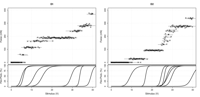
Figure 3: Stimulus-response curve (top) for the simulated data with lines representing the expected WMTF over the stimuli intervals where the joint firing probability is greater than 5% according to the individual excitability curves (bottom). Left: Data set D1 contains $u^{*}=7$ MUs but $\hat{u}=8$. Right: Data set D2 contains $u^{*}=8$ MUs but $\hat{u}=7$. Circle points, additional 23 simulations over the 23–32 V alternation period involving 5 MUs.

4.1 Over-estimation

The first data set, D1, contains $u^{*}=7$ MUs in truth but the SMC-MUNE method produces a MAP estimate of $\hat{u}=8$. The posterior probability of the true model is $\hat{p}_{u^{*}}=14.9\%$ and this model, along with the larger 9 MU model, is contained with a 95% HPCS. Parameter estimates for the MAP model (Table 2) show that the penultimate MU has a median expected twitch force of 9.6 mN with a credible upper bound of 15.7 mN, much lower than the 20 mN simulation threshold. Figure 4 presents the the construction of the predictive WMTF density for the true and MAP models at a 37 V stimulus. The local modes in the model containing the true MU-number correspond uniquely to particular firing combinations. In contrast, the weak MU in the MAP model principally serves to increase the variability around a specific WMTF response level rather than describing a distinct MU.

In light of these concerns, the marginal likelihood estimates are adjusted according to Section 3.4 with a conservative lower bound of $\mu_{\min}=15$ mN to guard against small MUs that, when firing, are indistinguishable from other combinations. The corrected posterior mass function places 89.3% of the mass on the correct, seven-MU model, with 10.7% mass on the eight-MU model. The estimates of expected MUTF in Table 2 for the seven-MU model are similar to those prior to the adjustment and are still close to the true values from which the data was generated. However, the prior adjustment for the eight-MU hypothesis has a significant effect on the penultimate MU and, so as to preserve the overall maximum WMTF, a small reduction in the estimated $\mu$s for its neighboring MUs.

Table 2: Expected MUTF median and 95% credible interval estimates for MUs with high excitation threshold from the true ($u^{*}=7$) and MAP ($\hat{u}=8$) models, with and without post-process truncation ($\mu_{\min}=15$ mN) on data set D1.

Parameter	$\mu_{6}$	$\mu_{7}$	$\mu_{8}$	$\nu^{-1}$
True	40.2 mN	87.9 mN	–	4.54  mN2
$u=7$	40.5 (37.7, 43.5)	91.2 (86.6, 95.9)	–	3.85 (3.13, 4.81)
$u=8$	36.3 (32.4, 40.2)	9.6 (4.7, 15.7)	86.7 (80.3, 92.7)	3.22 (2.57, 4.18)
$u=7$ & $\mu_{\min}=15$	40.5 (37.8, 40.2)	91.3 (86.8, 95.7)	–	3.90 (3.14, 4.92)
$u=8$ & $\mu_{\min}=15$	35.7 (31.1, 40.0)	15.7 (15.0, 20.7)	80.4 (71.4, 86.6)	3.23 (2.60, 4.09)

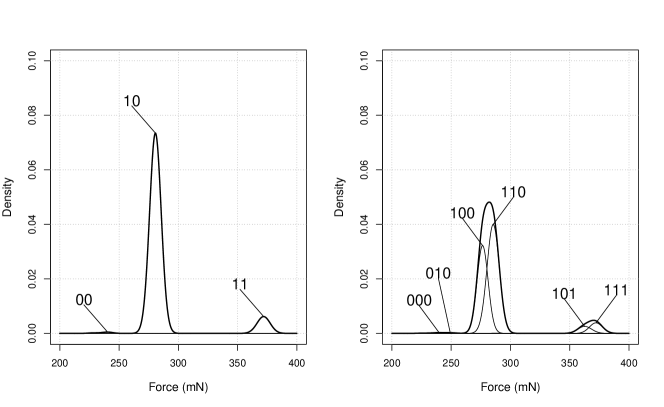
Figure 4: Predictive density (thick line) at stimulus 37 V from the seven (left) and eight (right) MU model without post-process adjustment. Thin lines identify the contribution to the predictive for the indicated firing combinations associated to the final few MUs. In both cases, the first five MUs fire with near certainty. Most firing combinations with negligible predictive probabilities are omitted from the plot.

4.2 Under-estimation

The second data set, D2, contains $u^{*}=8$ MUs and presents a period of alternation between 23–32 V which involves five MUs. The SMC-MUNE procedure, however, estimates $\hat{u}=7$ and gives this a high posterior probability of 97.1% after applying the post-process adjustment at $\mu_{\min}=15$ mN. The main source for this under-estimation arises through the over-estimation of the excitability scale parameter (Table 3) for the fourth MU ($\lambda_{4}$), so that the stimulus interval for probabilistic firing behavior is nearly three times wider than it should be. Consequently, this incorrectly estimated MU acts as a surrogate for MU-number $6$, which has similar twitch force properties.

One potential solution is to reduce the upper bound for the scale parameter $\lambda_{\max}$ in (4) to constrain estimation against shallow excitability curves. Table 3 presents scale parameter estimates for selected MUs at the original ($\lambda_{\max}=14$V) and reduced ($\lambda_{\max}=7$V) upper bounds. Under the reduced bound the 8 MU model becomes a member of the HPCS, but the MAP estimate remains at $\hat{u}=7$ with a high posterior probability of 94.6%. Although a further reduction to $\lambda_{\max}$ might be appealing, this action is likely to be detrimental in determining good model fits. For example, the scale parameter of the first MU, which has a true value of 5.0 V is accurately estimated whether $\lambda_{\max}$ is $7$ or $14$, principally because its excitability curve is well separated from the other curves, but a further reduction in $\lambda_{\max}$ risks the introduction of an additional, spurious MU to explain the low-stimulus observations.

Table 3: Motor unit posterior probabilities and excitation parameter estimates for selected MUs from D2 with scale upper bound at $\lambda_{\max}=14$ V and $\lambda_{\max}=7$ V, and with 23 additional measurements at $\lambda_{\max}=14$ V.

	True	$\lambda_{\max}=14$		$\lambda_{\max}=7$		Extra
$u$	8	7	8	7	8	7	8
$\mathbb{P}(u|y)$	–	96.7%	3.3%	94.6%	5.4%	28.7%	71.3%
$\eta_{4}$	26.0 V	26.9 (25.4, 28.8)	26.6 (25.3, 28.6)	27.0 (25.4, 28.9)	26.5 (25.2, 28.5)	26.7 (25.7, 27.7)	26.4 (25.6, 27.6)
$\eta_{5}$	27.3 V	27.8 (26.0, 29.1)	27.4 (25.5, 28.9)	27.8 (25.9, 29.0)	27.5 (25.6, 28.9)	27.4 (26.2, 28.5)	27.2 (25.9, 28.3)
$\eta_{6}$	27.9 V	–	27.9 (26.5, 29.5)	–	27.9 (26.6, 29.5)	–	27.5 (26.5, 28.8)
$\lambda_{4}$	1.8 V	4.5 (1.8, 7.6)	3.6 (1.0, 7.6)	4.3 (1.9, 6.6)	3.1 (0.7, 6.3)	4.0 (1.8, 7.8)	2.5 (0.9, 6.3)
$\lambda_{5}$	3.6 V	4.1 (2.2, 7.3)	4.7 (1.8, 7.9)	4.0 (2.1, 6.5)	4.4 (1.7, 6.6)	3.7 (2.1, 6.3)	4.6 (1.8, 8.3)
$\lambda_{6}$	4.8 V	–	4.7 (1.6, 8.1)	–	4.4 (1.4, 6.6)	–	4.4 (2.3, 7.5)

In the original analysis, $\lambda_{4}$ is mis-estimated because of the limited information available in the observations to adequately describe the period of alternation between 23–32 V which involves five MUs. To show that this is the case, an additional 23 observations were generated evenly over this interval; see Figure 3. This modest addendum to the data set is sufficient for the true model to be identified, $\hat{u}=8$, and with a posterior probability of 71.3%, and with better scale parameter estimates. However, the increase in computational resource required to obtain the same degree of Monte Carlo and numerical accuracy was substantial: from 5000 to 25000 particles and from a $30{\times}30$ to $50{\times}50$ lattice for the eight-MU hypothesis.

5 Case study: rat tibial muscle

The case study arises from (Casella et al., 2010) where a rat tibial muscle (medial gastrocnemius) receives stem cell therapy to encourage neuromuscular activation after simulating paralysis. The two data sets, presented in Figure 1, are generated by applying stimuli for different durations. The first data set, using 10µsec duration stimuli, consist of $T=304$ observations, including 11 baseline measurements and a maximal stimulus of 100 V. In contrast, the second data set was collected using 50µsec duration stimuli and consists of $T=669$ observations, including 7 baseline measurements, and with a maximal stimulus of 60 V. The data sets are named R10 and R50 respectively. Since both data sets are collected from the same neuromuscular system it is expected that MUNE should be similar between the data sets.

Naïve assessment of the stimulus-response curves by counting the number of distinct levels of twitch force suggests that there are perhaps nine or ten MUs, but this would ignore any potential features arising from alternation. The histogram inserts in Figure 1 present frequency in absolute difference between consecutive twitch forces when ordered by stimulus intensity. The highest frequency occurs at low differences and represents the within-MUTF variability whereas the less-frequent, larger differences appear due to the firing of different combinations of MUs. In both cases a minimum expected MUTF of $\mu_{\min}=15$ mN is suitable to correct against the estimation of MUs with negligible contribution to the observed twitch forces.

The SMC-MUNE procedure was applied up to a maximum model size of $u_{\max}=12$ with prior sufficient statistics and algorithmic parameters as specified in Appendix A. For both data sets, the estimated motor unit number posterior mass function (Table 4) identifies the MAP estimate as $\hat{u}=8$, with this being the only member of the HPCSs. There is a noticeable difference in the computational resources required as the MAP model for R50 required twenty times more particles and three times finer lattice than that for data set R10. This is in part reflective of the relative sizes of the data sets, but may also relate to the relative complexities of the state-spaces for the firing vectors.

Figure 5 presents the estimated excitability curves for each of the MUs, with MUs labelled in order of increasing $\mathbb{E}[\eta|y_{1:T}]$. First, the location parameters under the 50µsec duration stimuli are approximately four times lower than the corresponding parameters under 10µsec duration stimuli. This difference in scale corresponds to Weiss’s law (Bostock, 1983) that relates the excitation of the neuron to the charge built-up in the cell. Despite this, it is clear that the majority of the MUs are excited within a short stimulus window with only the last MU requiring a larger stimulus to be excited. This high degree of activity at low stimulus is reflective of the sudden early rise in the stimulus-response curves.

To compare MUs between data sets, the coefficient of variation for the random variable associated with each excitability curve is presented in Figure 5c. Apart from the first MU, the 95% credible intervals from each data set for a given MU overlap, suggesting similar coefficients of variation for the MUs; this might be anticipated since measurements are taken from the same neuromuscular system. These similar estimated coefficients are larger than the estimate in Hales et al. (2004), which is presented for comparison. This reflects the experimentation where the developed neurons are less stable and are yet to restore full and healthy motor function.

Table 5 present the most probable firing combinations for each visibly distinct response level in Figure 1. The estimated firing behavior of each MU, after label-swapping similarly excitable MUs for R50, are very similar between the two data sets. It can then be suggested that the level at approximately 120 mN in both data sets and at about 70 mN in R50 are potential consequences of alternation as MUs that fired in contributing to weaker WMTFs are latent in forming these response levels. However, a difference in estimated firing behavior occurs at the 120 mN response level whereby the SMC-MUNE procedure obtained two different model fits; MU1+MU4 in R10 and MU2+MU3 in R50. As a consequence, the estimated excitation range for MU1 in R50 is unusually large, leading to a relatively flat excitability curve with an enlarged coefficient of variation (Figure 5) in relation to other MUs and between data sets. Nevertheless, the net effect of these firing combinations with the estimated expected MUTFs, see Figure 5 inserts, does not suggest that the overall description of the two data sets greatly differ. This exemplifies the difficulty in disseminating between MUs with similar excitation and twitch characteristics. The difference in fit could have occurred in part due to the 70 mN response level in the R50 data set not being represented within dataset R10.

Data set	R10					R50
No. of MUs ($u$)	7	8	9	10		7	8	9	10
$\mathbb{P}(u|\mathbf{y})$ (%)	0.04	99.95	0.01	0.00		0.00	100.00	0.00	0.00
Grid Size ($n{\times}n$)	30	30	30	30		100	90	50	90
No. of Particles (,000s)	20	5	5	5		155	100	65	115

Table 4: Posterior summary from the SMC-MUNE procedure for the rat tibial muscle using 10µsec and 50µsec duration stimuli.

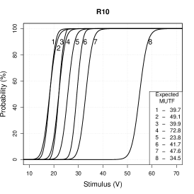
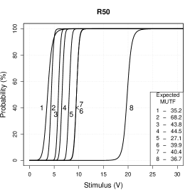
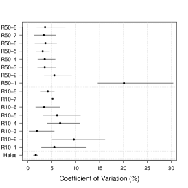
Figure 5: Estimated excitability curves from the eight MU hypotheses for data sets R10 (left) and R50 (centre) with corresponding expected MUTF mean estimates. Right: median and 95% credible interval for the coefficient of variation for the random variable associated with the excitability curve for each MU, together with the mean and 95% confidence interval from Hales et al..

Table 5: Most probable firing events (1=fire, 0=latent) for each level in the stimulus-response curve. The labeled MUs for R50 are re-ordered to demonstrate similarity between the two data sets. The response level around 70 mN is not present in the R10 data set.

	R10										R50
Level (mN)	1	2	3	4	5	6	7	8		Level (mN)	1	2	4	3	5	7	6	8
0	0	0	0	0	0	0	0	0		0	0	0	0	0	0	0	0	0
50	1	0	0	0	0	0	0	0		40	1	0	0	0	0	0	0	0
–	–	–	–	–	–	–	–	–		70	0	1	0	0	0	0	0	0
100	1	1	0	0	0	0	0	0		110	1	1	0	0	0	0	0	0
120	1	0	0	1	0	0	0	0		120	0	1	0	1	0	0	0	0
170	1	1	0	1	0	0	0	0		150	1	1	0	1	0	0	0	0
210	1	1	1	1	0	0	0	0		200	1	1	1	1	0	0	0	0
230	1	1	1	1	1	0	0	0		230	1	1	1	1	1	0	0	0
270	1	1	1	1	1	1	0	0		270	1	1	1	1	1	1	0	0
320	1	1	1	1	1	1	1	0		300	1	1	1	1	1	1	1	0
360	1	1	1	1	1	1	1	1		350	1	1	1	1	1	1	1	1

6 Discussion

This paper presents a new sequential Bayesian procedure for motor unit number estimation (MUNE), the assessment of the number of the operating motor units (MUs) from an electromyography investigation into muscle function. The fully adpated sequential Monte Carlo (SMC) filter uses the approximate conditional conjugacy of the twitch process. The principal purpose of SMC-MUNE is to estimate the marginal likelihood for the neuromuscular model based on a fixed number of MUs. From this, motor unit number estimation (MUNE) is then performed by comparing the evidence between competing MU-number hypotheses. As is demonstrated in Sections 4.1 and 4.2 SMC-MUNE also allows detailed scrutiny of the quality of each model fit.

SMC-MUNE performed well on simulated data, but two scenarios that may cause incorect estimation were identified. In the first scenario, one or more MUs were estimated to have a negligible or negative twitch force, allowing a model that was larger than the truth to fit the data and resulting in overestimation of the number of motor units (MUs). This lead to the development of a post-process correction that restricts the parameter space. By contrast, the second scenario resulted in under-estimation because of difficulty in estimating the underlying process during a period of alternation involving many MUs, where the same stimulus, applied repeatedly can lead to several different combinations of MUs firing. This issue persisted despite constraining a key parameter, but was resolved when, instead, additional data points were sampled from the region of alternation, strongly suggesting that the original underestimation arose because the information available in the data was not sufficient to fully characterise the firing process.

Independent application of SMC-MUNE to two data sets (with data collected as in Casella et al. (2010)) on the same neuromuscular system resulted in the same estimate for the number of MUs. However, closer examination of the model fits identifies minor variations in parameter estimates and firing patterns that reflected subtle and known differences between the two data sets.

The examples investigated in this paper involve neuromuscular systems with relatively small numbers of MUs. In practice, large and healthy muscle groups can contain hundreds of MUs (Gooch et al., 2014). Application of SMC-MUNE to these larger problems is currently impractical as the computation cost increases exponentially with the assumed number of MUs. As such the SMC-MUNE currently is best applied to small neuromuscular systems such as in some animal or in patients with amyotrophic lateral sclerosis who have limited motor function. The computational demand arises from the necessity to evaluate the predictive mass function for sampling the firing vectors and to marginalise this event space for calculating the resamping weights. One approach to address this is to approximate very low or very high excitation probabilities by their respective certainties as in Drovandi et al. (2014). Alternatively, the excitability curve for SMC-MUNE is specified in generic terms and so computational saving are possible by defining a function that has finite support. In addition to concerns over the size of the computation, additional resources would be required for a sufficiently fine lattice over the excitability parameter space to minimize numerical error on the marginal likelihood estimate. Although adaptive sparse grids (Bungartz and Dirnstorfer, 2003) have the potential to be more beneficial in terms of resource management and precision, care would be needed in automating the grid refinements, and it is likely that a unique grid would be associated with each distinct firing pattern.

The sequential aspect of the proposed methodology provides the opportunity for real-time inference that has the potential to provide in-lab assistance during experimentation. In this framework, an interim SMC-MUNE analysis could help in identifying the choice of stimulus to apply in order to collect the best evidence to distinguish between competing hypotheses, as in Section 4.2. The limitations of the present SMC-MUNE procedure to become a wholly online algorithm are the computational aspects discussed earlier and the post-processing stage to correct for potentially negligible estimates of the expected MU twitch forces. Solutions to these outstanding problems would increase the efficiency and accuracy of SMC-MUNE and, hence, the range of application.

Appendix A Additional detail

The prior sufficient statistics for the simulation and case studies are: $\bar{m}_{0}=0$, $\bar{c}_{0}=10^{3}$, $\bar{a}_{0}=0.5$, $\bar{b}_{0}=0.1$, $\mathbf{m}_{0}=40\mathbf{1}_{u}$, $C_{0}=10^{4}I_{u}$ and $a_{0}=0.5$ where $\mathbf{1}_{u}$ is a unit $u$-vector and $I_{u}$ is the $u\times{u}$ identity matrix. The statistic $b_{0}$ is defined according to (17) with $\delta=0.05$ and $\epsilon=0.2$. The upper bounds for the excitability parameter space are $\eta_{\max}=1.1s_{\tau}$ and $\lambda_{\max}=14$. In the case study, the upper bound for the scale parameter was reduced to $\lambda_{\max}=7$.

Resampling in Algorithm 1, is performed by systematic sampling on the residuals of particle weights (Hol et al., 2006). The number of particle samples and the number of rectangular lattice cells is initially $N=5000$ and $|\mathcal{G}|=30\times{30}$ respectively.

Accuracy in MU-number posterior mass function is managed by ensuring that for each model, $u$, the range in marginal log-likelihood estimate from 3 independent runs of the SMC scheme is less than $1$ whenever the posterior probability is greater than 1%. If not, then the particle set is increased in steps of $5000$ samples to reduce Monte Carlo variability. Once this criterion is satisfied, the lattice for the numerical integration is made finer by 10 vertices in both dimensions and the stability of the estimates to increasing grid size is checked; instability leads to a further check of the Monte Carlo variability and, if necessary, an increase in the particle set size, and then a further increase in the number of vertices; iteration between these two steps continues until the results are numerically stable and have a low variance. For a particular data set, once the minimal number of particles and grid size required for stability have been ascertained, a further $7$ runs are performed using these settings and the final marginal log-likelihood estimate is the average of the result from the total of $10$ runs.

References

- Andrieu (2007) C. Andrieu. Discussion of: Motor unit number estimation using reversible jump Markov chain Monte Carlo methods. Journal of the Royal Statistical Society. Series C. Applied Statistics, 56(3):261–263, 2007.
- Bostock (1983) H Bostock. The strength-duration relationship for excitation of myelinated nerve: computed dependence on membrane parameters. The Journal of Physiology, 341(1):59–74, 1983.
- Bromberg (2003) M. B. Bromberg. Consensus. Supplements to Clinical Neurophysiology, 55(C):333–338, 2003.
- Bromberg (2007) M. B. Bromberg. Updating motor unit number estimation (MUNE). Clinical neurophysiology, 118(1):1–8, 2007.
- Brown and Milner-Brown (1976) W. F. Brown and H. S. Milner-Brown. Some electrical properties of motor units and their effects on the methods of estimating motor unit numbers. Journal of Neurology, Neurosurgery & Psychiatry, 39(3):249–257, 1976.
- Bungartz and Dirnstorfer (2003) H.-J. Bungartz and S. Dirnstorfer. Multivariate quadrature on adaptive sparse grids. Computing, 71(1):89–114, 2003.
- Carvalho et al. (2010) C. M. Carvalho, M. S. Johannes, H. F. Lopes, and N. G. Polson. Particle learning and smoothing. Statistical Science. A Review Journal of the Institute of Mathematical Statistics, 25(1):88–106, 2010.
- Casella et al. (2010) G. T. B. Casella, V. W. Almeida, R. M. Grumbles, Y. Liu, and C. K. Thomas. Neurotrophic factors improve muscle reinnervation from embryonic neurons. Muscle & nerve, 42(5):788–797, 2010.
- Daube (1995) J. R. Daube. Estimating the number of motor units in a muscle. Journal of Clinical Neurophysiology, 12(6):585–594, 1995.
- Drovandi et al. (2014) C. C. Drovandi, A. N. Pettitt, R. D. Henderson, and P. A. McCombe. Marginal reversible jump Markov chain Monte Carlo with application to motor unit number estimation. Computational Statistics & Data Analysis, 72:128–146, 2014.
- Genz and Bretz (2009) A. Genz and F. Bretz. Computation of multivariate normal and probabilities, volume 195 of Lecture Notes in Statistics. Springer, Dordrecht, 2009.
- Gooch et al. (2014) C. L. Gooch, T. J. Doherty, K. M. Chan, M. B. Bromberg, R. A. Lewis, D. W. Stashuk, M. J. Berger, M. T. Andary, and J. R. Daube. Motor unit number estimation: a technology and literature review. Muscle & nerve, 50(6):884–893, 2014.
- Green (1995) P. J. Green. Reversible jump Markov chain Monte Carlo computation and Bayesian model determination. Biometrika, 82(4):711–732, 1995.
- Hales et al. (2004) J. P. Hales, C. S.-Y. Lin, and H. Bostock. Variations in excitability of single human motor axons, related to stochastic properties of nodal sodium channels. The Journal of physiology, 559(3):953–964, 2004.
- Henderson et al. (2006) R. D. Henderson, G. R. Ridall, A. N. Pettitt, P. A. McCombe, and J. R. Daube. The stimulus–response curve and motor unit variability in normal subjects and subjects with amyotrophic lateral sclerosis. Muscle & nerve, 34(1):34–43, 2006.
- Hol et al. (2006) J. D. Hol, T. B. Schon, and F. Gustafsson. On resampling algorithms for particle filters. In Nonlinear Statistical Signal Processing Workshop, 2006 IEEE, pages 79–82. IEEE, 2006.
- Kadrie et al. (1976) H. A. Kadrie, S. K. Yates, H. S. Milner-Brown, and W. F. Brown. Multiple point electrical stimulation of ulnar and median nerves. Journal of Neurology, Neurosurgery & Psychiatry, 39(10):973–985, 1976.
- Major and Jones (2005) L. A. Major and K. E. Jones. Simulations of motor unit number estimation techniques. Journal of neural Engineering, 2(2):17, 2005.
- Major et al. (2007) L. A. Major, J. Hegedus, D. J. Weber, T. Gordon, and K. E. Jones. Method for counting motor units in mice and validation using a mathematical model. Journal of neurophysiology, 97(2):1846–1856, 2007.
- McComas et al. (1971) A. J. McComas, P. Fawcett, M. J. Campbell, and R. E. P. Sica. Electrophysiological estimation of the number of motor units within a human muscle. Journal of Neurology, Neurosurgery & Psychiatry, 34(2):121–131, 1971.
- Pitt and Shephard (1999) M. K. Pitt and N. Shephard. Filtering via simulation: auxiliary particle filters. Journal of the American Statistical Association, 94(446):590–599, 1999.
- Ridall et al. (2006) P. G. Ridall, A. N. Pettitt, R. D. Henderson, and P. A. McCombe. Motor unit number estimation—a Bayesian approach. Biometrics, 62(4):1235–1250, 2006.
- Ridall et al. (2007) P. G. Ridall, A. N. Pettitt, N. Friel, P. A. McCombe, and R. D. Henderson. Motor unit number estimation using reversible jump Markov chain Monte Carlo methods. Journal of the Royal Statistical Society. Series C. Applied Statistics, 56(3):235–269, 2007.
- Shefner et al. (2006) J. M. Shefner, M. Cudkowicz, and R. H. Brown. Motor unit number estimation predicts disease onset and survival in a transgenic mouse model of amyotrophic lateral sclerosis. Muscle & nerve, 34(5):603–607, 2006.
- Stashuk et al. (1994) D. W. Stashuk, T. J. Doherty, A. Kassam, and W. F. Brown. Motor unit number estimates based on the automated analysis of F-responses. Muscle & nerve, 17(8):881–890, 1994.