The Multigaussian method: a new approach to multichannel radiochromic film dosimetry
Abstract
Abstract:
The main objective of multichannel radiochromic film dosimetry methods is to correct, or at least mitigate, spatial heterogeneities in the film-scanner response, especially variations in the active layer thickness. To this end, films can also be scanned prior to irradiation. In this study, the abilities of various single channel and multichannel methods to reduce spatial heterogeneities, with and without scanning before irradiation, were tested. A new approach to multichannel dosimetry, based on experimental findings, i.e., the Multigaussian method, is introduced. The Multigaussian method assumes that the probability density function of the response vector formed by the pixel values of the different color channels, including irradiated and non-irradiated scans, follows a multivariate Gaussian distribution. The Multigaussian method provided more accurate doses than the other models under comparison, especially when incorporating the information of the film prior to irradiation.
I Introduction
Small fields, steep dose gradients or regions without electronic equilibrium are some of the many situations in which radiation doses can be measured using radiochromic films. Particular strengths of radiochromic films are weak energy dependence Rink, Vitkin, and Jaffray (2007); Richter et al. (2009); Arjomandy et al. (2010); Lindsay et al. (2010); Massillon-JL et al. (2012); Bekerat et al. (2014), near water-equivalence Crijns et al. (2013); Niroomand-Rad et al. (1998), and high spatial resolution. On the other hand, the dosimetry system composed of radiochromic films and a flatbed scanner suffers from several sources of uncertainty, which can affect the film (e.g., differences in the active layer thickness Hartmann, Martišíková, and Jäkel (2010), evolution of film darkening with post-irradiation time Andrés et al. (2010); Chang et al. (2014), dependency on humidity and temperature Rink et al. (2008), noncatalytic and ultraviolet-catalyzed polymerization Girard, Bouchard, and Lacroix (2012), scratches), the scanner (e.g., the warming-up of the lamp Paelinck, Neve, and Wagter (2007); Ferreira, Lopes, and Capela (2009), inter-scan variations Lewis and Devic (2015); Méndez et al. (2016), noise Bouchard et al. (2009); van Hoof et al. (2012), dust), or the interaction between film and scanner (e.g., the lateral artifact Schoenfeld et al. (2014); van Battum et al. (2015); Schoenfeld et al. (2016), the dependency on the orientation of the film on the scanner bed Butson, Cheung, and Yu (2009), the dependency on film-to-light source distance Lewis and Devic (2015); Palmer, Bradley, and Nisbet (2015), Newton rings Dreindl, Georg, and Stock (2014), the cross talk effect van Battum et al. (2015)). Film handling and scanning protocols Niroomand-Rad et al. (1998); Bouchard et al. (2009), corrections Lewis et al. (2012); Méndez et al. (2013); Lewis and Devic (2015); Lewis and Chan (2015); Méndez et al. (2016); Ruiz-Morales, Vera-Sánchez, and González-López (2017) and multichannel dosimetry methods Micke, Lewis, and Yu (2011); Mayer et al. (2012); Méndez et al. (2014); Azorín, García, and Martí-Climent (2014) have been developed to reduce uncertainties and deliver precise and accurate doses Palmer, Nisbet, and Bradley (2013); Vera-Sánchez, Ruiz-Morales, and González-López (2018).
Multichannel radiochromic film dosimetry methods combine the information provided by all three color channels (R, G and B) of the scanner. In order to do so, the perturbation of the film-scanner response caused by different sources of uncertainty must be (explicitly or implicitly) modeled. Current multichannel methods assume that changes in the response for the different channels are positively correlated. Moreover, perturbations should be small. For example, even though the lateral artifact produces positively correlated perturbations (i.e., pixel values decrease with the distance from the center of the scan for all three channels, given a constant dose), these perturbations increase with the dose and the distance from the center, eventually becoming excessive for multichannel models Schoenfeld et al. (2016). The primary targets of multichannel film dosimetry are the spatial heterogeneities of the response and, in particular, differences in the active layer thickness. These differences can also be addressed by incorporating the information of the film prior to irradiation employing net optical density (NOD) as the film-scanner response.
The purpose of this study was to select the most accurate method for mitigating spatial heterogeneities in the response. The effectiveness of NOD and various multichannel models was compared with a novel approach to multichannel radiochromic film dosimetry which we have called the Multigaussian method.
II Methods and materials
II.1 Measurements
Commonly, multichannel models are evaluated using the gamma index: a sample of clinical plans are calculated with the treatment planning system (TPS) and posteriorly irradiated, dose distributions are computed with each multichannel model and the multichannel model that produces dose distributions which are most similar to the TPS doses according to the gamma index is deemed to be the most accurate model Méndez et al. (2014); Azorín, García, and Martí-Climent (2014); Méndez (2015). Film corrections are also examined in a similar fashion Menegotti, Delana, and Martignano (2008); Palmer, Bradley, and Nisbet (2015). This procedure has several drawbacks Clasie et al. (2012): apart from the accuracy of the multichannel model, the gamma index depends on the shape of the dose distribution in the individual plans, the noise in the distributions, the tolerance criteria, the interpolation method implemented for the gamma index computation, the choice of reference and evaluation dose distributions, the accuracy of the TPS, etc.
In this work, the measurement protocol was designed with the aim of minimizing the influence of any source of uncertainty other than the spatial heterogeneity of the response. Two lots of Gafchromic EBT3 films (lots 06061401 and 04071601) and one lot of EBT-XD films (lot 12101501) were employed. They were identified as lots A, B and C, respectively. The dosimetry system was completed with an Epson Expression 10000XL flatbed scanner (Seiko Epson Corporation, Nagano, Japan) and the scanning software Epson Scan v3.49a. Five films per lot were scanned prior to and 24 h following irradiation. Irradiation was delivered with a 6 MV beam from a Novalis Tx accelerator (Varian, Palo Alto, CA, USA). Films were positioned at source-axis distance (SAD) on top of the IBA MatriXX detector (IBA Dosimetry GmbH, Germany) inside the IBA MULTICube phantom. Doses were simultaneously measured with the MatriXX detector. Field dimensions were 2020 for lot A and 2525 for lots B and C. Films were irradiated with 1, 2, 4, 8 and 16 Gy for lots A and B, and 2, 4, 8, 16 and 32 Gy for lot C. In this setup, 1 Gy corresponded to 109 MU.
Before use, the scanner was warmed up for at least 30 min. Films were centered on the scanner bed with a transparent frame. In order to correct inter-scan variations, a 20.324.50 unexposed fragment was kept in a constant position and scanned together with the films. Films were scanned in portrait orientation (i.e., the scanner lamp was parallel to the short side of the film). The distance between film and lamp was kept constant by placing a 3 mm thick glass sheet on top of the film Lewis and Devic (2015); Palmer, Bradley, and Nisbet (2015). Scans were acquired in transmission mode with a resolution of 50 dpi. Processing tools were disabled. Ten scans were taken for each film, the first five were discarded and the resulting image was the median of the remaining five scans. Images were saved as 48-bit RGB format (16 bit per channel) TIFF files.
II.2 Data set
From the measurements, each pixel of each film was associated with a position , three (R, G and B) pixel values (PVs) prior to irradiation, three PVs after irradiation, and the dose measured with MatriXX at that position. MatriXX dose arrays, which have a resolution of 7.62 mm/px, were bicubically interpolated to the resolution of the films. In order to avoid large dose gradients, which are associated with higher uncertainties, points with a measured dose lower than 95% of the nominal dose were excluded from the set. Data analysis was implemented in the R environment R Core Team (2012).
Inter-scan and lateral corrections were applied on irradiated and non-irradiated PVs. Inter-scan variations were corrected using the unexposed fragment, following the column correction method Méndez et al. (2016). Lateral corrections were applied according to the model
| (1) |
where represents the PV before the lateral correction, is the coordinate on the axis parallel to the lamp, is the position of the center of the scanner, and are corrected PVs Méndez et al. (2013); Lewis and Chan (2015). The images of unexposed films can facilitate the determination of the parameters in this equation. If we symbolize with and the PV as a function of of unexposed films before and after applying lateral corrections, we can rewrite the model as
| (2) |
Apart from being trivially obtained, another advantage of using and is that they are robust against variations in the active layer, since they can be calculated from the average (or median) of several films. For each color channel, and in equation 2 were fitted from the median of the film scans prior to irradiation, and the parameters were derived from the irradiated films. The corrected PVs () are necessary for computing the parameters. Corrected PVs were derived from measured doses. The relationship between PVs and measured doses (i.e., the calibration) was calculated using regions of interest (ROIs) with dimensions 33 centered on the fields. Sensitometric and inverse sensitometric curves for all three color channels were modeled with natural cubic splines.
Therefore, apart from the positions, measured irradiated PVs, measured non-irradiated PVs, and measured doses, the data set included PVs after applying inter-scan corrections and PVs after applying inter-scan and lateral corrections.
II.3 The Multigaussian method
Perturbations of the response in radiochromic film dosimetry can be expressed as
| (3) |
where denotes the calibration function for color channel , is the film-scanner response at point , and is the perturbation.
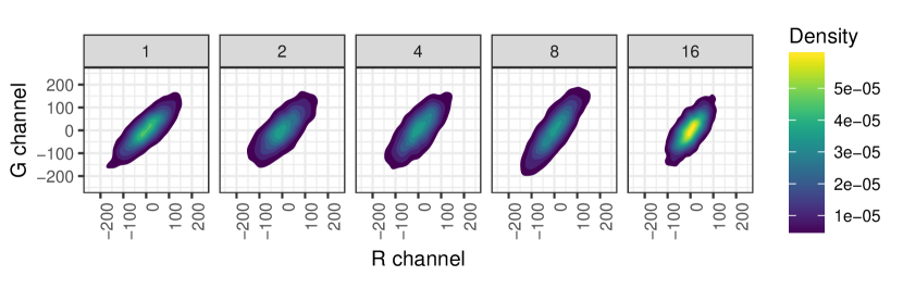
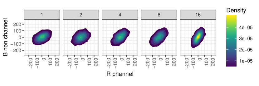
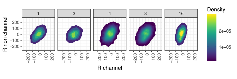
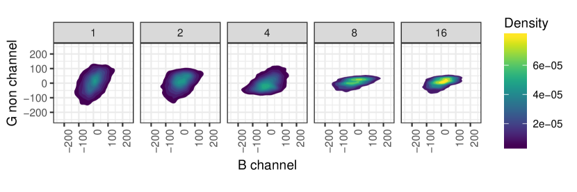
Figure 1 shows the plots of the joint probabilities of perturbations (i.e., ) for different combinations of color channels and different doses. The perturbations are calculated as the differences between the mean PV and the PV of each point in the ROIs used for the calibration. Measured PVs were analyzed prior to irradiation (channels R non, G non and B non) and after irradiation (channels R, G and B). For illustration purposes, only four combinations of channels using the films from lot A are shown. However, every possible combination of channels for every lot and film was examined. It can be observed that the perturbations are small (in general, lower than 2% of the response) and positively correlated, and that the joint probabilities might be approximated with bivariate Gaussian distributions. This behavior points to a novel approach to radiochromic film dosimetry: the Multigaussian method.
The Multigaussian method considers that, given a dose , the probability of the response vector (i.e., the vector with the responses for each channel) obeys a multivariate Gaussian distribution
| (4) |
Here, is the number of different channels (i.e., irradiated channels and optionally non-irradiated channels), is the vector of expected values of the response and is the covariance matrix
| (5) |
During the calibration, and can be measured for a set of doses. For the remaining doses, they should be interpolated. In this study, we interpolated and with natural cubic splines.
Following a Bayesian approach, the probability of each dose given a response vector can be computed as
| (6) |
where the prior probabilities of are considered to be equiprobable.
Therefore, given a response , the dose (or more precisely the probability density function of the dose) can be obtained by
| (7) |
II.4 Model selection
The Multigaussian method was compared with other multichannel and single channel film dosimetry models. The relevance of scanning before irradiation was also evaluated. The Multigaussian method can integrate the information from the film prior to irradiation as additional dimensions of the response vector () in terms of PVs. In this work, the Multigaussian method was applied with and without non-irradiated channels, and the other models were calculated both with PVs and NODs as response. The additional use of optical density (OD) was discarded since there is only a change of coordinates between PV and OD. NOD was computed as
| (8) |
where indicates the PVs of the irradiated film, and indicates the PVs of the film prior to irradiation.
Many models were compared, but for the sake of clarity, only the most successful of them are analyzed here. The best results with single channel models were obtained using the red (R) channel. While, among the multichannel models, the most successful were the Mayer model Mayer et al. (2012) and what we called the Normal Factor model.
The Mayer model considers that the perturbation is additive and approximately equal for all channels:
| (9) |
where symbolizes the error term. The perturbation is presumed to be small. Thus, a first-order Taylor expansion of the dose in terms of the channel independent perturbation yields
| (10) |
where is the first derivative of with respect to and is an error term. Different assumptions about the probability density functions (PDFs) of or lead to different estimations of the dose Méndez et al. (2014). The Mayer model considers that the PDF of is a uniform distribution and that all follow the same normal distribution.The most likely value of the dose () in the Mayer model is calculated as
| (11) |
The Normal Factor model assumes a multiplicative perturbation which is approximately equal for all channels:
| (12) |
Again, different PDFs for or give rise to different dose distributions. In the Normal Factor model, all follow the same normal distribution (i.e., ), but the PDF of is also normal (i.e., ). In this case, the most likely value of the dose is
| (13) |
where is the ratio . The best results for the Normal Factor model were obtained with , which is roughly the square of the mean PV, meaning that both and contributed to the perturbation with similar weight. In order to calculate the dose , it can be deduced from equation 13 that, given ,
| (14) |
and
| (15) |
where is obtained from the calibration .
III Results and discussion
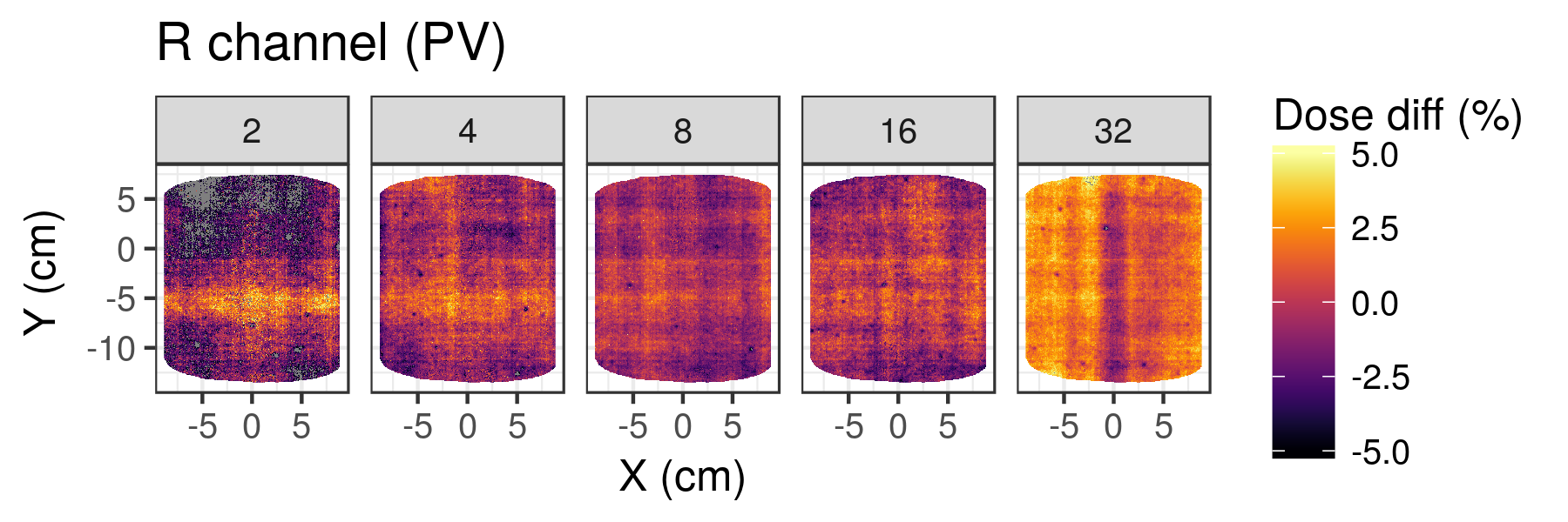
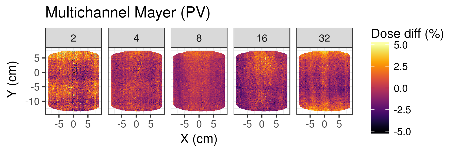
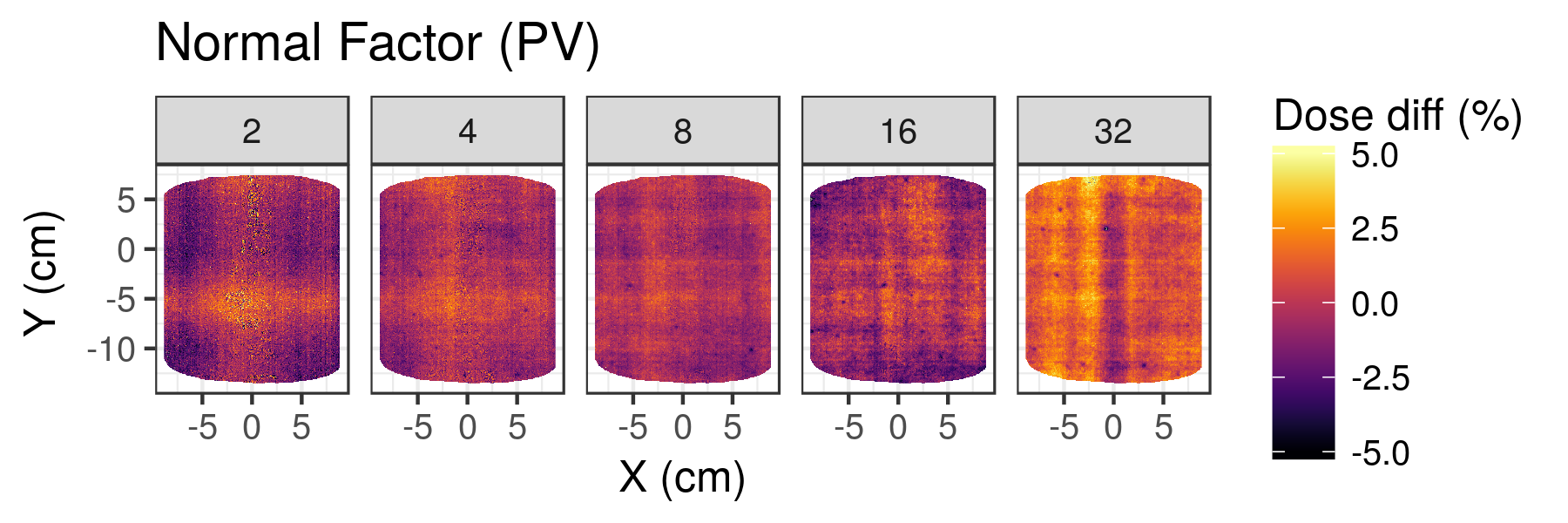
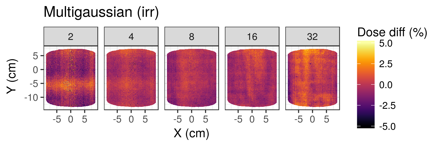
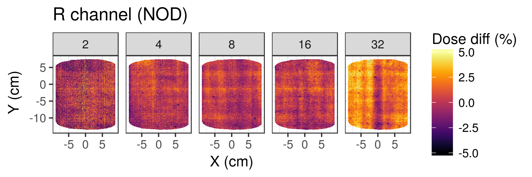
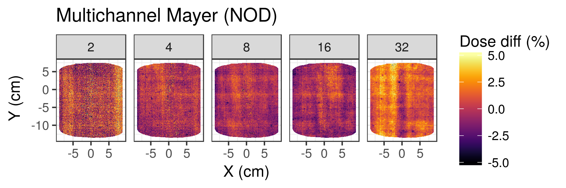
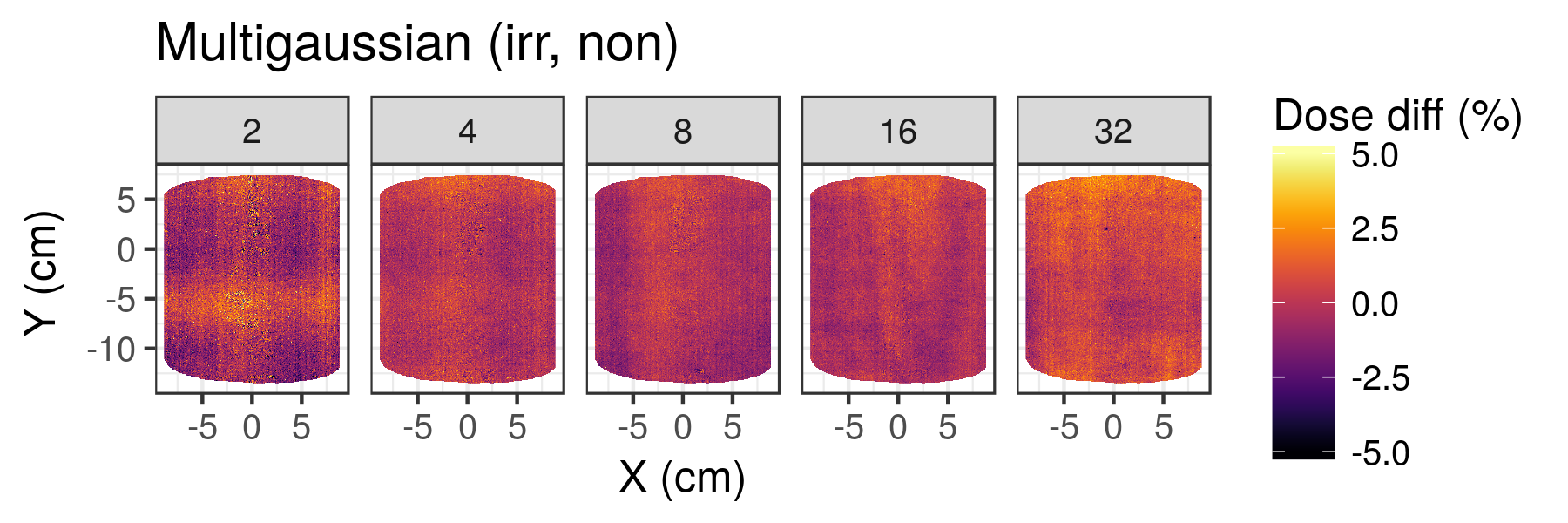
Figure 2 and figure 3 show the relative dose differences between measured doses with MatriXX and doses calculated with each dosimetry model. In figure 2, irradiated PVs were employed as the response. In figure 3, the Multigaussian model used both irradiated and non-irradiated PVs and the rest of the models employed NODs. In both figures, inter-scan and lateral corrections were applied. Although only films from lot C are shown, all three lots produced similar outcomes. Table 1 condenses this information into the standard deviation of the dose difference between measured and calculated doses for each lot.
It can be observed that the Multigaussian model delivered more accurate doses. However, no method corrects spatial heterogeneities completely. Low frequency heterogeneities, presumably due to active layer variations, are still visible González-López, Vera-Sánchez, and Ruiz-Morales (2017). Whether using only the scans of irradiated films, or including the scans prior to irradiation, and for each lot under study, the Multigaussian model gave lower dose differences than the other three models. Scanning prior to and after irradiation improved the results of the Multigaussian and R channel models, but this was not true for all lots when employing the Mayer or Normal Factor models. Therefore, in this study, the most accurate film dosimetry model for mitigating spatial heterogeneities was the Multigaussian method scanning prior to and after irradiation.

| Film dosimetry method | Lot A | Lot B | Lot C |
|---|---|---|---|
| R channel (PV) | 1.7 | 2.3 | 2.0 |
| Multichannel Mayer (PV) | 1.6 | 2.4 | 1.4 |
| Factor Normal (PV) | 1.6 | 1.7 | 1.3 |
| Multigaussian (irr) | 1.4 | 1.4 | 1.1 |
| R channel (NOD) | 1.2 | 1.7 | 1.6 |
| Multichannel Mayer (NOD) | 1.6 | 2.0 | 1.8 |
| Factor Normal (NOD) | 1.3 | 1.8 | 1.6 |
| Multigaussian (irr, non) | 1.1 | 1.2 | 1.0 |
Table 2 shows how uncertainties increase when lateral corrections are not applied. In this case, however, it should be noted that giving a unique value for the standard deviation of the dose differences is not informative enough, since the differences increase with the dose and the distance from the center. In spite of this, the results support the recommendation of applying lateral corrections even with multichannel film dosimetry methods.
| Film dosimetry method | Lot A | Lot B | Lot C |
|---|---|---|---|
| R channel (PV) | 4.0 | 4.4 | 3.2 |
| Multichannel Mayer (PV) | 2.0 | 2.1 | 1.9 |
| Factor Normal (PV) | 2.5 | 2.9 | 2.1 |
| Multigaussian (irr) | 2.0 | 2.6 | 1.5 |
| R channel (NOD) | 3.5 | 3.5 | 2.5 |
| Multichannel Mayer (NOD) | 3.6 | 4.2 | 2.9 |
| Factor Normal (NOD) | 1.9 | 2.4 | 2.1 |
| Multigaussian (irr, non) | 1.5 | 2.0 | 1.3 |
IV Conclusions
The purpose of this work was to select the method which best reduces spatial heterogeneities in radiochromic film dosimetry. The design of the experiment aimed to minimize any other sources of uncertainty. Single channel and multichannel methods, including a novel multichannel approach to film dosimetry called the Multigaussian method, were compared. The convenience of scanning both prior to and after irradiation was examined also.
The Multigaussian method provided more accurate doses than the other models. The best results were obtained with the Multigaussian method integrating the information from the film before irradiation. This information is not integrated as net optical density but as additional elements in the response vector, which is composed of the pixel values of the different color channels including irradiated and non-irradiated scans. The assumption of the Multigaussian method is that the probability density function of the response vector follows a multivariate Gaussian distribution. This assumption is based on empirical findings.
Although the Multigaussian method obtained the best agreement between doses measured with film and MatriXX, spatial heterogeneities, presumably caused by variations in the active layer thickness, are still present. Therefore, new and more accurate multichannel radiochromic film dosimetry methods are necessary. This research demonstrates a new way of tackling the problem.
Acknowledgements.
I. Méndez is co-founder of Radiochromic.com.References
- Rink, Vitkin, and Jaffray (2007) A. Rink, I. A. Vitkin, and D. A. Jaffray, “Energy dependence (75 kVp to 18 MV) of radiochromic films assessed using a real-time optical dosimeter,” Medical Physics 34, 458–463 (2007).
- Richter et al. (2009) C. Richter, J. Pawelke, L. Karsch, and J. Woithe, “Energy dependence of EBT-1 radiochromic film response for photon (10 kVp–15 MVp) and electron beams (6–18 MeV) readout by a flatbed scanner,” Medical Physics 36, 5506–5514 (2009).
- Arjomandy et al. (2010) B. Arjomandy, R. Tailor, A. Anand, N. Sahoo, M. Gillin, K. Prado, and M. Vicic, “Energy dependence and dose response of Gafchromic EBT2 film over a wide range of photon, electron, and proton beam energies,” Medical Physics 37, 1942–1947 (2010).
- Lindsay et al. (2010) P. Lindsay, A. Rink, M. Ruschin, and D. Jaffray, “Investigation of energy dependence of EBT and EBT-2 Gafchromic film,” Medical Physics 37, 571–576 (2010).
- Massillon-JL et al. (2012) G. Massillon-JL, S. Chiu-Tsao, I. Domingo-Munoz, and M. Chan, “Energy Dependence of the New Gafchromic EBT3 Film:Dose Response Curves for 50 KV, 6 and 15 MV X-Ray Beams,” International Journal of Medical Physics, Clinical Engineering and Radiation Oncology 1, 60–65 (2012).
- Bekerat et al. (2014) H. Bekerat, S. Devic, F. DeBlois, K. Singh, A. Sarfehnia, J. Seuntjens, S. Shih, X. Yu, and D. Lewis, “Improving the energy response of external beam therapy (EBT) GafChromic dosimetry films at low energies ( 100 keV),” Medical Physics 41, 022101 (14pp.) (2014).
- Crijns et al. (2013) W. Crijns, F. Maes, U. A. van der Heide, and F. V. den Heuvel, “Calibrating page sized Gafchromic EBT3 films,” Medical Physics 40, 012102 (13pp.) (2013).
- Niroomand-Rad et al. (1998) A. Niroomand-Rad, C. R. Blackwell, B. M. Coursey, K. P. Gall, J. M. Galvin, W. L. McLaughlin, A. S. Meigooni, R. Nath, J. E. Rodgers, and C. G. Soares, “Radiochromic film dosimetry: Recommendations of AAPM Radiation Therapy Committee Task Group 55,” Medical Physics 25, 2093–2115 (1998).
- Hartmann, Martišíková, and Jäkel (2010) B. Hartmann, M. Martišíková, and O. Jäkel, “Technical Note: Homogeneity of Gafchromic EBT2 film,” Medical Physics 37, 1753–1756 (2010).
- Andrés et al. (2010) C. Andrés, A. del Castillo, R. Tortosa, D. Alonso, and R. Barquero, “A comprehensive study of the Gafchromic EBT2 radiochromic film. A comparison with EBT,” Medical Physics 37, 6271–6278 (2010).
- Chang et al. (2014) L. Chang, S.-Y. Ho, H.-J. Ding, T.-F. Lee, and P.-Y. Chen, “Dependency of EBT2 film calibration curve on postirradiation time,” Medical physics 41 (2014).
- Rink et al. (2008) A. Rink, D. F. Lewis, S. Varma, I. A. Vitkin, and D. A. Jaffray, “Temperature and hydration effects on absorbance spectra and radiation sensitivity of a radiochromic medium,” Medical physics 35, 4545–4555 (2008).
- Girard, Bouchard, and Lacroix (2012) F. Girard, H. Bouchard, and F. Lacroix, “Reference dosimetry using radiochromic film,” Journal of Applied Clinical Medical Physics 13 (2012).
- Paelinck, Neve, and Wagter (2007) L. Paelinck, W. D. Neve, and C. D. Wagter, “Precautions and strategies in using a commercial flatbed scanner for radiochromic film dosimetry,” Physics in Medicine and Biology 52, 231–242 (2007).
- Ferreira, Lopes, and Capela (2009) B. Ferreira, M. Lopes, and M. Capela, “Evaluation of an Epson flatbed scanner to read Gafchromic EBT films for radiation dosimetry,” Physics in medicine and biology 54, 1073 (2009).
- Lewis and Devic (2015) D. Lewis and S. Devic, “Correcting scan-to-scan response variability for a radiochromic film-based reference dosimetry system,” Medical physics 42, 5692–5701 (2015).
- Méndez et al. (2016) I. Méndez, Ž. Šljivić, R. Hudej, A. Jenko, and B. Casar, “Grid patterns, spatial inter-scan variations and scanning reading repeatability in radiochromic film dosimetry,” Physica Medica 32, 1072–1081 (2016).
- Bouchard et al. (2009) H. Bouchard, F. Lacroix, G. Beaudoin, J.-F. Carrier, and I. Kawrakow, “On the characterization and uncertainty analysis of radiochromic film dosimetry,” Medical Physics 36, 1931–1946 (2009).
- van Hoof et al. (2012) S. J. van Hoof, P. V. Granton, G. Landry, M. Podesta, and F. Verhaegen, “Evaluation of a novel triple-channel radiochromic film analysis procedure using EBT2,” Physics in Medicine and Biology 57, 4353–4368 (2012).
- Schoenfeld et al. (2014) A. A. Schoenfeld, D. Poppinga, D. Harder, K.-J. Doerner, and B. Poppe, “The artefacts of radiochromic film dosimetry with flatbed scanners and their causation by light scattering from radiation-induced polymers,” Physics in Medicine and Biology 59, 3575–3597 (2014).
- van Battum et al. (2015) L. van Battum, H. Huizenga, R. Verdaasdonk, and S. Heukelom, “How flatbed scanners upset accurate film dosimetry,” Physics in medicine and biology 61, 625 (2015).
- Schoenfeld et al. (2016) A. A. Schoenfeld, S. Wieker, D. Harder, and B. Poppe, “The origin of the flatbed scanner artifacts in radiochromic film dosimetry-key experiments and theoretical descriptions,” Physics in medicine and biology 61, 7704 (2016).
- Butson, Cheung, and Yu (2009) M. J. Butson, T. Cheung, and P. Yu, “Evaluation of the magnitude of EBT Gafchromic film polarization effects,” Australasian Physics & Engineering Sciences in Medicine 32, 21–25 (2009).
- Palmer, Bradley, and Nisbet (2015) A. L. Palmer, D. A. Bradley, and A. Nisbet, “Evaluation and mitigation of potential errors in radiochromic film dosimetry due to film curvature at scanning,” Journal of Applied Clinical Medical Physics 16 (2015).
- Dreindl, Georg, and Stock (2014) R. Dreindl, D. Georg, and M. Stock, “Radiochromic film dosimetry: Considerations on precision and accuracy for EBT2 and EBT3 type films,” Zeitschrift für Medizinische Physik 24, 153–163 (2014).
- Lewis et al. (2012) D. Lewis, A. Micke, X. Yu, and M. F. Chan, “An efficient protocol for radiochromic film dosimetry combining calibration and measurement in a single scan,” Medical Physics 39, 6339–6350 (2012).
- Méndez et al. (2013) I. Méndez, V. Hartman, R. Hudej, A. Strojnik, and B. Casar, “Gafchromic EBT2 film dosimetry in reflection mode with a novel plan-based calibration method,” Medical Physics 40, 011720 (9pp.) (2013).
- Lewis and Chan (2015) D. Lewis and M. F. Chan, “Correcting lateral response artifacts from flatbed scanners for radiochromic film dosimetry,” Medical physics 42, 416–429 (2015).
- Ruiz-Morales, Vera-Sánchez, and González-López (2017) C. Ruiz-Morales, J. A. Vera-Sánchez, and A. González-López, “On the re-calibration process in radiochromic film dosimetry,” Physica Medica: European Journal of Medical Physics 42, 67–75 (2017).
- Micke, Lewis, and Yu (2011) A. Micke, D. F. Lewis, and X. Yu, “Multichannel film dosimetry with nonuniformity correction,” Medical Physics 38, 2523–2534 (2011).
- Mayer et al. (2012) R. R. Mayer, F. Ma, Y. Chen, R. I. Miller, A. Belard, J. McDonough, and J. J. O’Connell, “Enhanced dosimetry procedures and assessment for EBT2 radiochromic film,” Medical Physics 39, 2147–2155 (2012).
- Méndez et al. (2014) I. Méndez, P. Peterlin, R. Hudej, A. Strojnik, and B. Casar, “On multichannel film dosimetry with channel-independent perturbations,” Medical Physics 41, 011705 (10pp.) (2014).
- Azorín, García, and Martí-Climent (2014) J. F. P. Azorín, L. I. R. García, and J. M. Martí-Climent, “A method for multichannel dosimetry with EBT3 radiochromic films,” Medical Physics 41, 062101 (10pp.) (2014).
- Palmer, Nisbet, and Bradley (2013) A. L. Palmer, A. Nisbet, and D. Bradley, “Verification of high dose rate brachytherapy dose distributions with EBT3 Gafchromic film quality control techniques,” Physics in medicine and biology 58, 497 (2013).
- Vera-Sánchez, Ruiz-Morales, and González-López (2018) J. A. Vera-Sánchez, C. Ruiz-Morales, and A. González-López, “Monte carlo uncertainty analysis of dose estimates in radiochromic film dosimetry with single-channel and multichannel algorithms,” Physica Medica 47, 23–33 (2018).
- Méndez (2015) I. Méndez, “Model selection for radiochromic film dosimetry,” Physics in medicine and biology 60, 4089 (2015).
- Menegotti, Delana, and Martignano (2008) L. Menegotti, A. Delana, and A. Martignano, “Radiochromic film dosimetry with flatbed scanners: A fast and accurate method for dose calibration and uniformity correction with single film exposure,” Medical Physics 35, 3078–3085 (2008).
- Clasie et al. (2012) B. M. Clasie, G. C. Sharp, J. Seco, J. B. Flanz, and H. M. Kooy, “Numerical solutions of the gamma-index in two and three dimensions,” Physics in Medicine and Biology 57, 6981–6997 (2012).
- R Core Team (2012) R Core Team, R: A Language and Environment for Statistical Computing, R Foundation for Statistical Computing, Vienna, Austria (2012), ISBN 3-900051-07-0.
- González-López, Vera-Sánchez, and Ruiz-Morales (2017) A. González-López, J. A. Vera-Sánchez, and C. Ruiz-Morales, “The incidence of the different sources of noise on the uncertainty in radiochromic film dosimetry using single channel and multichannel methods,” Physics in Medicine & Biology 62, N525 (2017).