Time Evolution of an Infinite Projected Entangled Pair State:
an Algorithm from First Principles

Abstract

A typical quantum state obeying the area law for entanglement on an infinite 2D lattice can be represented by a tensor network ansatz – known as an infinite projected entangled pair state (iPEPS) – with a finite bond dimension $D$. Its real/imaginary time evolution can be split into small time steps. An application of a time step generates a new iPEPS with a bond dimension $k$ times the original one. The new iPEPS does not make optimal use of its enlarged bond dimension $kD$, hence in principle it can be represented accurately by a more compact ansatz, favourably with the original $D$. In this work we show how the more compact iPEPS can be optimized variationally to maximize its overlap with the new iPEPS. To compute the overlap we use the corner transfer matrix renormalization group (CTMRG). By simulating sudden quench of the transverse field in the 2D quantum Ising model with the proposed algorithm, we provide a proof of principle that real time evolution can be simulated with iPEPS. A similar proof is provided in the same model for imaginary time evolution of purification of its thermal states.

I Introduction

Tensor networks are a natural language to represent quantum states of strongly correlated systemsVerstraete et al. (2008); Orús (2014). Among them the most widely used ansatze are a matrix product states (MPS) Fannes et al. (1992) and its 2D generalization: pair-entangled projected state (PEPS) Verstraete and Cirac (2004) also known as a tensor product state. Both obey the area law for entanglement entropy. In 1D matrix product states are efficient parameterizations of ground states of gapped local Hamiltonians Verstraete et al. (2008); Hastings (2007); Schuch et al. (2008) and purifications of thermal states of 1D local Hamiltonians Barthel (2017). MPS is the ansatz optimized by the density matrix renormalization group (DMRG) White (1992, 1993) which is one of the most powerful methods to simulate not only ground states of 1D systems but also theirs exited states, thermal states or dynamic properties Schollwöck (2005); Schöllwock (2011).

PEPS are expected to be an efficient parametrization of ground states of 2D gapped local Hamiltonians Verstraete et al. (2008); Orús (2014) and were shown to be an efficient representation of thermal states of 2D local Hamiltonians Molnar et al. (2015), though in 2D there are limitations to the assumed representability of area-law states by tensor networks Ge and Eisert (2016). Furthermore tensor networks can be used to represent efficiently systems with fermionic degrees of freedom Pineda et al. (2010); Corboz and Vidal (2009); Barthel et al. (2009); Gu et al. (2010) as was demonstrated for both finite Kraus et al. (2010) and infinite PEPS Corboz et al. (2010, 2011).

PEPS was originally proposed as a varaitional ansatz for ground states of 2D finite systems Verstraete and Cirac (2004); Murg et al. (2007) generalizing earlier attempts to construct trial wave-functions for specific 2D models using 2D tensor networks Nishio et al. (2004). Efficient numerical methods enabling optimisation and controlled approximate contraction of infinite PEPS (iPEPS) Jordan et al. (2008); Jiang et al. (2008); Gu et al. (2008); Orús and Vidal (2009) became basis for promising new methods for strongly correlated systems. Among recent achievements of those methods are solution of a long standing magnetization plateaus problem in highly frustrated compound $\textrm{SrCu}_{2}(\textrm{BO}_{3})_{2}$ Matsuda et al. (2013); Corboz and Mila (2014) and obtaining coexistence of superconductivity and striped order in the underdoped regime of the Hubbard model – a result which is corroborated by other numerical methods (among them another tensor network approach - DMRG simulations of finite-width cylinders) – apparently settling one of long standing controversies concerning that model Zheng et al. (2017). Another example of a recent contribution of iPEPS-based methods to condensed matter physics is a problem of existence and nature of spin liquid phase in kagome Heisenberg antiferromagnet for which new evidence in support of gapless spin liquid was obtained Liao et al. (2017). This progress was accompanied and partly made possible by new developments in iPEPS optimization Corboz (2016a); Vanderstraeten et al. (2016), iPEPS contraction Fishman et al. (2017); Xie et al. (2017); Czarnik et al. (2016a), energy extrapolations Corboz (2016b), and universality class estimation Corboz et al. (2018); Rader and Läuchli (2018); Rams et al. (2018). These achievements encourage attempts to use iPEPS to simulate broad class of states obeying 2D area law like thermal states Czarnik et al. (2012); Czarnik and Dziarmaga (2014, 2015a); Czarnik et al. (2016b); Czarnik and Dziarmaga (2015b); Czarnik et al. (2016a, 2017); Dai et al. (2017), states of dissipative systems Kshetrimayum et al. (2017) or exited states Vanderstraeten et al. (2015).

Among alternative tensor network approaches to strongly correlated systems are methods of direct contraction and renormalization of a 3D tensor network representing a density operator of a 2D thermal state Li et al. (2011); Xie et al. (2012); Ran et al. (2012, 2013, 2018); Peng et al. (2017); Chen et al. (2017) and, technically challenging yet able to represent critical states with subleading logarithmic corrections to the area law, multi-scale entanglement renormalization ansatz (MERA) Vidal (2007, 2008) and its generalization branching MERA Evenbly and Vidal (2014a, b). Recent years brought also progress in using DMRG to simulate cylinders with finite width. Such simulations are routinely used alongside iPEPS to investigate 2D systems ground states (see e.g. Ref. Zheng et al., 2017) and were applied recently also to thermal states Bruognolo et al. (2017); Chen et al. (2018).

In this work we test an algorithm to simulate either real or imaginary time evolution with iPEPS. The algorithm uses second order Suzuki-Trotter decomposition of the evolution operator into small time steps Trotter (1959); Suzuki (1966, 1976). A straightforward application of a time step creates a new iPEPS with a bond dimension $k$ times the original bond dimension $D$. If not truncated, the evolution would result in an exponential growth of the bond dimension. Therefore, the new iPEPS is approximated variationally by an iPEPS with the original $D$. The algorithm is a straightforward construction directly from first principles with a minimal number of approximations controlled by the iPEPS bond dimension $D$ and the environmental bond dimension $\chi$ in CTMRG. It uses CTMRG Baxter (1978); Nishino and Okunishi (1996); Orús and Vidal (2009); Corboz et al. (2014) to compute fidelity between the new iPEPS and its variational approximation. The very calculation of fidelity between two close iPEPS was shown to be tractable only very recently Jahromi et al. (2018). In this work we go further and demonstrate that the fidelity can be optimized variationally effectively enough for time evolution.

A challenging application of the method is real time evolution after a sudden quench. A sudden quench of a parameter in a Hamiltonian excites entangled pairs of quasiparticles with opposite quasimomenta that run away from each other crossing the boundary of the subsystem. Consequently, the number of pairs that are entangled across the boundary (proportional to the entanglement entropy) grows linearly with time requiring an exponential growth of the bond dimension. Therefore, a tensor network is doomed to fail after a finite evolution time. Nevertheless, matrix product states proved to be useful for simulating time evolution after sudden quenches in 1D Halimeh and Zauner-Stauber (2017). As a proof of principle that the same can be attempted with iPEPS in 2D, in this work we simulate a sudden quench in the transverse field quantum Ising model.

Moreover, there are other – easier from the entanglement point of view – potential applications of the real time variational evolution. For instance, a smooth ramp of a parameter in a Hamiltonian across a quantum critical point generates the entanglement entropy proportional to the area of the boundary times a logarithm of the Kibble-Zurek correlation length $\hat{\xi}$ that in turn is a power of the ramp time Cincio et al. (2007). Thanks to this dynamical area law, the required $D$ instead of growing exponentially with time saturates becoming a power of the ramp time. Even stronger limitations may apply in many-body localization (MBL), where localized excitations are not able to spread the entanglement. Tensor networks have already been applied to 2D MBL phenomena Wahl et al. (2017). Finally, after vectorization of the density matrix, the unitary time evolution can be generalized to a Markovian master equation with a Lindblad superoperator, where local decoherence limits the entanglement making the time evolution with a tensor network feasible Werner et al. (2016); Kshetrimayum et al. (2017).

Another promising application is imaginary time evolution generating thermal states of a quantum Hamiltonian. By definition, a thermal Gibbs state maximizes entropy for a given average energy. As this maximal entropy is the entropy of entanglement of the system with the rest of the universe, then – by the monogamy of entanglement – there is little entanglement left inside the system. In more quantitative terms, both thermal states of local Hamiltonians and iPEPS representations of density operators obey area law for mutual information making an iPEPS a good ansatz for thermal states Wolf et al. (2008). In this paper we evolve a purification of thermal states in the quantum Ising model obtaining results convergent to the variational tensor network renormalization (VTNR) introduced and applied to a number of models in Czarnik and Dziarmaga (2015b); Czarnik et al. (2016b, a, 2017). This test is a proof of principle that thermal states can be obtained with the variational imaginary time evolution.

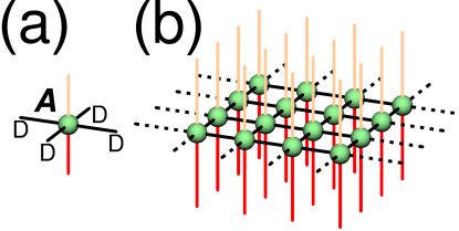
Figure 1: In a, an elementary rank-6 tensor $A$ of a purification. The top (orange) index numbers ancilla states $a=0,1$, the bottom (red) index numbers spins states $s=0,1$, the four (black) bond indices have a bond dimension $D$. In b, an iPEPS representation of the purification. Here pairs of elementary tensors at NN lattice sites were contracted through their connecting bond indices. The whole network is an amplitude for a joint spins’ and ancillas’ state labelled by the open spin and ancilla indices. Reducing the dimension of ancilla indices to 1 (or simply ignoring the ancilla lines) we obtain a well known iPEPS representation of a pure state.

The paper is organized as follows. In section II we introduce purification of a thermal state to be evolved in imaginary time. In section III we introduce the algorithm in the more general case of imaginary time evolution of a thermal state purification. A modification to real time evolution of a pure state is straightforward. In subsection III.1 we make Suzuki-Trotter decomposition of a small time step and represent it by a tensor network. In subsection III.2 we outline the algorithm whose further details are refined in subsections III.3,III.4, and appendix A. In section IV the algorithm is applied to simulate imaginary time evolution generating thermal states. Its results are compared with VTNR. In section V the real time version of the algorithm is tested in the challenging problem of time evolution after a sudden quench. Finally, we conclude in section VI.

II Purification of thermal states

We will exemplify the general idea with the transverse field quantum Ising model on an infinite square lattice

$$H~{}=~{}-\sum_{\langle j,j^{\prime}\rangle}Z_{j}Z_{j^{\prime}}-\sum_{j}\left(h_{x}X_{j}+h_{z}Z_{j}\right).$$ (1)

Here $Z,X$ are Pauli matrices. At zero longitudinal bias, $h_{z}=0$, the model has a ferromagnetic phase with a non-zero spontaneous magnetization $\langle Z\rangle$ for sufficiently small transverse field $h_{x}$ and sufficiently large inverse temperature $\beta$. At $h_{x}=0$ the critical $\beta$ is $\beta_{0}=-\ln(\sqrt{2}-1)/2\approx 0.441$ and at zero temperature the quantum critical point is $h_{0}=3.04438(2)$ Blöte and Deng (2002).

In an enlarged Hilbert space, every spin with states $s=0,1$ is accompanied by an ancilla with states $a=0,1$. The space is spanned by states $\prod_{j}|s_{j},a_{j}\rangle$, where $j$ is a lattice site. The Gibbs operator at an inverse temperature $\beta$ is obtained from its purification $|\psi(\beta)\rangle$ (defined in the enlarged space) by tracing out the ancillas,

$$\rho(\beta)\propto e^{-\beta H}={\rm Tr}_{\rm ancillas}|\psi(\beta)\rangle\langle\psi(\beta)|.$$ (2)

At $\beta=0$ we choose a product over lattice sites,

$$|\psi(0)\rangle=\prod_{j}~{}\sum_{s=0,1}|s_{j},s_{j}\rangle,$$ (3)

to initialize the imaginary time evolution

$$|\psi(\beta)\rangle~{}=~{}e^{-\frac{1}{2}\beta H}|\psi(0)\rangle~{}=~{}U(-i\beta/2)|\psi(0)\rangle.$$ (4)

The evolution operator $U(\tau)=e^{-i\tau H}$ acts in the Hilbert space of spins. With the initial state (3) Eq. (2) becomes

$$\rho(\beta)~{}\propto~{}U(-i\beta/2)U^{\dagger}(-i\beta/2).$$ (5)

Just like a pure state of spins, the purification can be represented by a iPEPS, see Fig. 1.

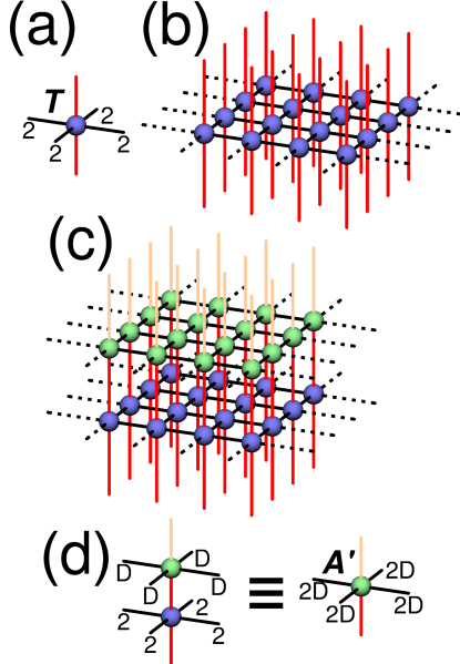
Figure 2: In a, an elementary rank-6 Trotter tensor $T$ with two (red) spin indices and four (black) bond indices, each of dimension 2. In b, a layer of Trotter tensors representing a small time step $U(d\tau)$. In c, the time step $U(d\tau)$ is applied to spin indices of the purification. In d, the tensors $T$ and $A$ can be contracted into a single new tensor $A^{\prime}$. A layer of $A^{\prime}$ makes a new iPEPS that looks like the original one in Fig. 1b but has a doubled bond dimension $2D$.

III The Method

We introduce the algorithm in the more general case of thermal states simulation by imaginary time evolution of their purification. To be more specific, we use the example of the quantum Ising model. Modification to real time evolution amounts to ignoring any ancilla lines in the diagrams. For the sake of clarity, in the main text we fully employ the symmetry of the Ising model but we do our numerical simulations with a more efficient algorithm, described in Appendix A, that breaks the symmetry by applying 2-site nearest-neighbor gates. That algorithm can be generalized to less symmetric models in a straightforward manner.

III.1 Suzuki-Trotter decomposition

In the second-order Suzuki-Trotter decomposition a small time step is

$$U(d\tau) = U_{h}(d\tau/2)U_{ZZ}(d\tau)U_{h}(d\tau/2),$$ (6)

where

$$U_{ZZ}(d\tau)=\prod_{\langle j,j^{\prime}\rangle}e^{id\tau Z_{j}Z_{j^{\prime}}},~{}U_{h}(d\tau)=\prod_{j}e^{id\tau h_{j}}$$ (7)

are elementary gates and $h_{j}=h_{x}X_{j}+h_{z}Z_{j}$.

In order to rearrange $U(d\tau)$ as a tensor network, we use singular value decomposition to rewrite a 2-site term $e^{id\tau Z_{j}Z_{j^{\prime}}}$ acting on a NN bond as a contraction of 2 smaller tensors acting on single sites:

$$e^{id\tau Z_{j}Z_{j^{\prime}}} = \sum_{\mu=0,1}z_{j,\mu}z_{j^{\prime},\mu}.$$ (8)

Here $\mu$ is a bond index and $z_{j,\mu}\equiv\sqrt{\Lambda_{\mu}}\,(Z_{j})^{\mu}$ and $\Lambda_{0}=\cos d\tau$ and $\Lambda_{1}=i\sin d\tau$. Now we can write

$$U(d\tau) = \sum_{\{\mu\}}\prod_{j}\left[e^{id\tau h_{j}/2}\left(\prod_{j^{\prime}}z_{j,\mu_{\langle j,j^{\prime}\rangle}}\right)e^{id\tau h_{j}/2}\right].$$ (9)

Here $\mu_{\langle j,j^{\prime}\rangle}$ is a bond index on the NN bond $\langle j,j^{\prime}\rangle$ and $\{\mu\}$ is a collection of all such bond indices. The square brackets enclose a Trotter tensor $T(d\tau)$ at site $j$, see Fig. 2a. It is a spin operator depending on the bond indices connecting its site with its four NNs. A contraction of these Trotter tensors is the gate $U(d\tau)$ in Fig. 2b. The evolution operator is a product of such time steps, $U(Nd\tau)=\left[U(d\tau)\right]^{N}$.

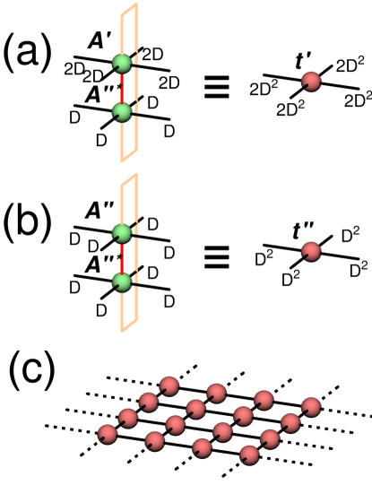
Figure 3: In a, tensor $A^{\prime}$ is contracted with a complex conjugate of $A^{\prime\prime}$ into a transfer tensor $t^{\prime}$ with a bond dimension $d=2D^{2}$. In b, tensor $A^{\prime\prime}$ is contracted with its own complex conjugate into a transfer tensor $t^{\prime\prime}$ with a bond dimension $d=D^{2}$. In c, an infinite layer of tensors $t^{\prime}$ ($t^{\prime\prime}$) represents the overlap $\langle\psi^{\prime\prime}|\psi^{\prime}\rangle$ ($\langle\psi^{\prime\prime}|\psi^{\prime\prime}\rangle$).

III.2 Variational truncation

The time step $U(d\tau)$ applied to the state $|\psi\rangle$ yields a new state

$$|\psi^{\prime}\rangle=U(d\tau)|\psi\rangle,$$ (10)

see Figs. 2c and d. If $|\psi\rangle$ has a bond dimension $D$, then the new iPEPS has twice the original bond dimension $2D$.

In order to prevent exponential growth of the dimension in time, the new iPEPS has to be approximated by a more compact one, $|\psi^{\prime\prime}\rangle$, made of tensors $A^{\prime\prime}$ with the original bond dimension $D$. The best $|\psi^{\prime\prime}\rangle$ minimizes the norm

$$\left||\psi^{\prime\prime}\rangle-|\psi^{\prime}\rangle\right|^{2}.$$ (11)

Equivalently – up to normalization of $|\psi^{\prime\prime}\rangle$ – the quality of the approximation can be measured by a global fidelity

$$F=\frac{\langle\psi^{\prime\prime}|\psi^{\prime}\rangle\langle\psi^{\prime}|\psi^{\prime\prime}\rangle}{\langle\psi^{\prime\prime}|\psi^{\prime\prime}\rangle}.$$ (12)

After a rearrangement in section III.3 below, it becomes an efficient figure of merit.

The iPEPS tensor $A^{\prime\prime}$ – the same at all sites – has to be optimized globally. However, the first step towards this global optimum is a local pre-update. We choose a site $j$ and label the tensor at this site as $A^{\prime\prime}_{j}$. This tensor is optimized while all other tensors are kept fixed as $A^{\prime\prime}$. With the last constraint the norm (11) becomes a quadratic form in $A^{\prime\prime}_{j}$. The quadratic form is minimized with respect to $A^{\prime\prime}_{j}$ by $\tilde{A}$ that solves the linear equation

$$G\tilde{A}=V.$$ (13)

Here

$$G=\frac{\partial^{2}\langle\psi^{\prime\prime}|\psi^{\prime\prime}\rangle}{\partial\left(A^{\prime\prime}_{j}\right)^{*}\partial\left(A^{\prime\prime}_{j}\right)},~{}~{}V=\frac{\partial\langle\psi^{\prime\prime}|\psi^{\prime}\rangle}{\partial\left(A^{\prime\prime}_{j}\right)^{*}}$$ (14)

are, respectively, a metric tensor and a gradient. Further details on the local pre-update can be found in section III.4 below.

The global fidelity (12) is not warranted to increase when the local optimum $\tilde{A}$ is substituted globally, i.e., in place of every $A^{\prime\prime}$ at every lattice site. However, $\tilde{A}$ can be used as an estimate of the most desired direction of the change of $A^{\prime\prime}$. In this vein, we attempt an update

$$A^{\prime\prime}=A\cos\epsilon+\tilde{A}\sin\epsilon,$$ (15)

with an adjustable parameter $\epsilon\in[-\pi/2,\pi/2]$ using an algorithm proposed in Ref. Corboz, 2016a which simplified version was introduced in Refs. Nishino et al., 2001; Gendiar et al., 2003. This update was successfully used in a similar variational problem of minimizing energy of an iPEPS as a function of $A$ Corboz (2016a), where we refer for its detailed account. Here we just sketch the general idea.

To begin with, the global fidelity $F_{0}$ is calculated for the “old” tensor $A^{\prime\prime}=A$ with $\epsilon=0$. For small $\epsilon$ the optimization is prone to get trapped in a local optimum. This is why large $\epsilon=\pi/2$ is tried first and if $F>F_{0}$ then $A^{\prime\prime}=\tilde{A}$ is accepted. Otherwise, $\epsilon$ is halved as many times as necessary for $F$ to increase above $F_{0}$ and then $A^{\prime\prime}=\tilde{A}$ is accepted. Negative $\epsilon$ are also considered in case the global $F$ does not increase for a positive $\epsilon$.

Once $A^{\prime\prime}$ in (15) is accepted, the whole procedure beginning with a solution of (13) is iterated until $F$ is converged. The final converged $A^{\prime\prime}$ is accepted as a global optimum.

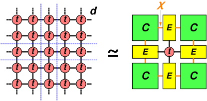
Figure 4: Left, planar version of Fig. 3c. Right, its approximate representation with corner tensors $C$ and edge tensors $E$. Here $C$ effectively represents a corner of the infinite graph on the left and $E$ its semi-infinite edge. Environmental bond dimension $\chi$ controls accuracy of the approximation. Tensors $C$ and $E$ are obtained with corner transfer matrix renormalization group Baxter (1978); Nishino and Okunishi (1996); Orús and Vidal (2009); Corboz et al. (2014).

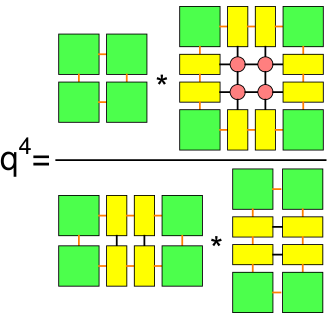
Figure 5: The environmental tensors introduced in Fig. 4 can be used to calculate the figure of merit (17). This diagram shows a fourth power of a factor $q$ by which the diagram in Fig. 3c (or, equivalently, the left panel of Fig. 4) is multiplied when $4$ sites are added to the network. Depending on the overlap in question – either $\langle\psi^{\prime\prime}|\psi^{\prime}\rangle$ or $\langle\psi^{\prime\prime}|\psi^{\prime\prime}\rangle$, see Fig. 3 – the factor is either $n=q$ or $d=q$, respectively. The diagram is equivalent to Fig.13.9 in R. J. Baxter’s textbook Baxter (1982).

III.3 Efficient fidelity computation

In the limit of infinite lattice, the overlaps in the fidelity (12) become

$$\langle\psi^{\prime\prime}|\psi^{\prime}\rangle=\lim_{N\to\infty}n^{N},~{}~{}\langle\psi^{\prime\prime}|\psi^{\prime\prime}\rangle=\lim_{N\to\infty}d^{N},$$ (16)

where $N$ is the number of lattice sites. Consequently, the fidelity becomes $F=\lim_{N\to\infty}f^{N},$ where

$$f=\frac{nn^{*}}{d}$$ (17)

is a figure of merit per site.

The factors $n$ and $d$ can be computed by CTMRGJahromi et al. (2018) generalizing the CTMRG approach to compute a partition function per site for 2D statistical models Baxter (1978, 1982); ban Chan (2012, 2013). First of all, each overlap – either $\langle\psi^{\prime\prime}|\psi^{\prime}\rangle$ or $\langle\psi^{\prime\prime}|\psi^{\prime\prime}\rangle$ – can be represented by a planar network in Fig. 3c. With the help of CTMRG Baxter (1978); Nishino and Okunishi (1996); Orús and Vidal (2009); Corboz et al. (2014), this infinite network can be effectively replaced by a finite one, as shown in Fig. 4. Figure 5 shows how to obtain $n$ and $d$ with the effective environmental tensors introduced in Fig. 4.

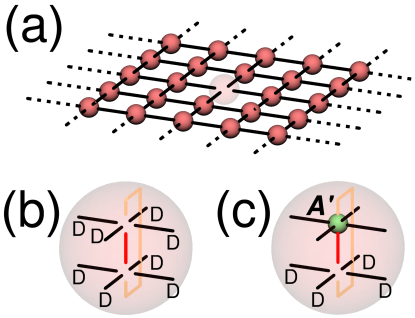
Figure 6: In a, tensor environment for $t^{\prime}$ ($t^{\prime\prime}$). It is obtained by removing one tensor $t^{\prime}$ ($t^{\prime\prime}$) from the overlap in Fig. 3c or equivalently from the right diagram in Fig. 4. The environment represents a derivative of the overlap $\langle\psi^{\prime\prime}|\psi^{\prime}\rangle$ ($\langle\psi^{\prime\prime}|\psi^{\prime\prime}\rangle$) with respect to $t^{\prime}$ ($t^{\prime\prime}$) (18,19). This rank-4 tensor has 4 indices with dimension $D\times 2D$ ($D\times D$), respectively. In b, in case of $t^{\prime\prime}$ (18) each of the 4 indices in (a) is decomposed back into two indices, each of dimension $D$. The diagram represents the metric tensor $G$. The open (red) spin line is a Kronecker delta for spin states and the open (orange) ancilla line is a delta for ancillas. Therefore, the metric can be decomposed as $G=g\otimes 1_{s}\otimes 1_{a}$, where $g$ is the tensor environment for $t$. In c, in case of $t^{\prime}$ (19) each of the 4 indices in (a) is decomposed back into two indices of dimension $2D$ (upper) and $D$ (lower). After contracting the upper indices with $A^{\prime}$ the diagram becomes the gradient $V$.

III.4 Local pre-update

In order to construct $G$ and $V$ from the effective environmental tensors $C$ and $T$, it is useful to note first that a derivative of a contraction of two rank-$n$ tensors $f=\sum_{i_{1},...,i_{n}}A_{i_{1},...,i_{n}}B_{i_{1},...,i_{n}}$ with respect to one of them gives the other one: $\partial f/\partial A_{i_{1},...,i_{n}}=B_{i_{1},...,i_{n}}$. Futhermore, we note that both the optimized tensor $A^{\prime\prime}_{j}$ and its conjugate $\left(A^{\prime\prime}_{j}\right)^{*}$ are located at the same site $j$ and they enter the overlap $\langle\psi^{\prime\prime}|\psi^{\prime\prime}\rangle$ ($\langle\psi^{\prime\prime}|\psi^{\prime}\rangle$) only through the tensor $t^{\prime\prime}$ ($t^{\prime}$)defined in Fig. 3 (3a), located at this site. We distinguish this tensor $t^{\prime\prime}$ ($t^{\prime}$) by an index $j$ and call it $t^{\prime\prime}_{j}$ ($t^{\prime}_{j}$). Therefore, the derivatives in Eq. (14) decompose into a tensor contraction of derivatives

$$G = \frac{\partial\langle\psi^{\prime\prime}|\psi^{\prime\prime}\rangle}{\partial t^{\prime\prime}_{j}}\frac{\partial^{2}t^{\prime\prime}_{j}}{\partial\left(A^{\prime\prime}_{j}\right)^{*}\partial\left(A^{\prime\prime}_{j}\right)},$$ (18)

$$V = \frac{\partial\langle\psi^{\prime\prime}|\psi^{\prime}\rangle}{\partial t^{\prime}_{j}}\frac{\partial t^{\prime}_{j}}{\partial\left(A^{\prime\prime}_{j}\right)^{*}}$$ (19)

The derivatives of the overlaps with respect to $t^{\prime}_{j}$ ($t^{\prime\prime}_{j}$) are represented by Fig. 6a, where one tensor $t^{\prime}_{j}$ ($t^{\prime\prime}_{j}$) at site $j$ was removed from the overlap shown in Figs. 3c, 4. Indeed, a contraction of the missing $t^{\prime}_{j}$ ($t^{\prime\prime}_{j}$) with its environment in Fig. 6a through corresponding indices gives back the overlap. Diagramatically, this contraction amounts to filling the hole in Fig. 6a with the missing $t^{\prime}_{j}$ ($t^{\prime\prime}_{j}$). In numerical calculations, the infinite diagram in Fig. 6a is approximated by a equivalent finite one in a similar way as in Fig. 4.

The rank-4 tensor in Fig. 6a is a tensor environment for $t^{\prime}_{j}$ ($t^{\prime\prime}_{j}$). Each of its 4 indices is a concatenation of two iPEPS bond indices, one from the ket and one from the bra iPEPS layer and has a dimension equal to ($2D\times D$) $D\times D$. After splitting each index back into ket and bra indices, this environment can be used to calculate ($V$) $G$, as shown in Fig. 6c (Fig. 6b). In Fig. 6b the hole in Fig. 6a (with split ket and bra indices) is filled with the second derivative of $t^{\prime\prime}_{j}$ with respect to $A^{\prime\prime}_{j}$ and $\left(A^{\prime\prime}_{j}\right)^{*}$. Similarly as the derivative of an overlap with respect to $t^{\prime\prime}_{j}$, this derivative is obtained from the tensor $t^{\prime\prime}_{j}$ in Fig. 3b by removing both $A^{\prime\prime}_{j}$ and $\left(A^{\prime\prime}_{j}\right)^{*}$ from the diagram. In Fig. 6c the hole in Fig. 6a is filled by the derivative of $t^{\prime}_{j}$ with respect to $\left(A^{\prime\prime}_{j}\right)^{*}$. This derivative is obtained from the tensor $t^{\prime}_{j}$ in Fig. 3a by removing $\left(A^{\prime\prime}_{j}\right)^{*}$ from the diagram.

We have to keep in mind that the evironmental tensors are converged with limited precision that is usually set by demanding that local observables are converged with precision $\simeq 10^{-8}$. This precision limits the accuracy to which the matrix $G$ is Hermitean and positive definite. In order to avoid numerical instabilities this error has to filtered out by elliminating the anti-Hermitean part of $G$ and then truncating its eigenvalues that are less than a fraction of its maximal eigenvalue. The fraction is usually set at $10^{-8}$. To this end we solve the linear equation (13) using the Moore-Penrose pseudo-inverse

$$\tilde{A}={\rm pinv}(G)V,$$ (20)

where the truncation is implemented by setting an appropriate tolerance in the pseudo-inverse procedure.

Another advantage of the pseudo-inverse solution is that it does not contain any zero modes of $G$. By definition, these zero modes do not matter for the local optimization problem but they can make futile the attempt in (15) to use $\tilde{A}$ as a significant part of the global solution.

A possibility of further simplification occurs in Fig. 6b, where the open spin and ancilla lines represent two Kronecker symbols. The symbols are identities in the spin and ancilla subspace and, therefore, the metric $G$ has a convenient tensor-product structure $G=g\otimes 1_{s}\otimes 1_{a}$, where $g$ is a reshaped tensor environment for $t^{\prime\prime}_{j}$ and $1_{s}$ and $1_{a}$ are identities for spins and ancillas, respectively. Therefore – after appropriate reshaping of tensors – Eq. (20) can be reduced to

$$\tilde{A}={\rm pinv}(g)V,$$ (21)

where only the small tensor environment $g$ has to be pseudo-inverted.

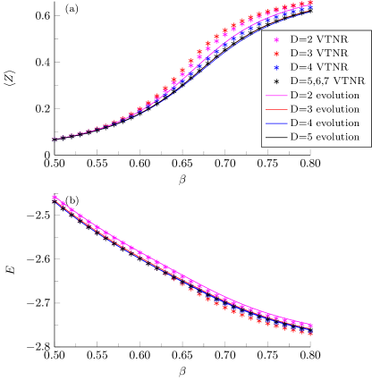
Figure 7: Thermal states for a transverse field $h_{x}=2.5$ with a longitudinal bias $h_{z}=0.01$. The stars are results from variational tensor network renormalization (VTNR) and the solid lines from the imaginary time evolution. With increasing bond dimension $D$ the two methods converge to each other. In a, longitudinal magnetization $\langle Z\rangle$ in function of inverse temperature. In b, energy per site $E$ in function of inverse temperature.

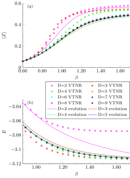
Figure 8: Thermal states for a transverse field $h_{x}=2.9$ with a longitudinal bias $h_{z}=0.01$. The stars are results from variational tensor network renormalization (VTNR) and the solid lines from the imaginary time evolution. With increasing bond dimension $D$ the two methods converge to each other. In a, longitudinal magnetization $\langle Z\rangle$ in function of inverse temperature. In b, energy per site $E$ in function of inverse temperature.

IV Thermal states from imaginary time evolution

In this section we present results obtained by imaginary time evolution for two values of the transverse field $h_{x}=2.5$ and $h_{x}=2.9$, see Figures 7 and 8, corresponding to critical temperatures $\beta_{c}=0.7851(4)$ and $\beta_{c}=1.643(2)$, respectively Hesselmann and Wessel (2016). We show data with $D=2,3,4,5$. The stronger field is closer to the quantum critical point at $h_{0}$, hence quantum fluctuations are stronger and a bigger bond dimension $D$ is required to converge. For the evolution to run smoothly across the critical point we added a small longitudinal bias $h_{z}=0.01$.

Figures 7a and 7b show the longitudinal magnetization $\langle Z\rangle$ and energy $E$ for the two transverse fields. The data from the evolution are compared to results obtained with the variational tensor network renormalization (VTNR) Czarnik and Dziarmaga (2015b); Czarnik et al. (2016b, a, 2017). With increasing $D$ each of the two methods converges and they converge to each other. This is a proof of principle that the variational time evolution can be applied to thermal states.

The data at hand suggest that with increasing $D$ the evolution converges faster than VTNR. However, at least for the Ising benchmark, numerical effort necessary to obtain results of similar accuracy is roughly the same. In both methods the bottleneck is the corner transfer matrix renormalization procedure. In the case of VTNR larger D is necessary but in the case of the evolution the environmental tensors need to be computed more times.

The advantage of VTNR is that it targets the desired temperature directly, there is no need to evolve from $\beta=0$ and thus no evolution errors are accumulated. In order to minimize the accumulation when evolving across the critical regime a small longitudinal bias has to be applied. The critical singularity is recovered in the limit of small bias that requires large $D$. However, one big advantage of the variational evolution is that – unlike VTNR targeting the accuracy of the partition function – it aims directly at an accurate thermal state. In some models this may prove to be a major advantage.

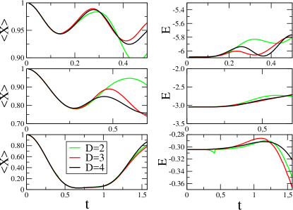
Figure 9: Transverse magnetization $\langle X\rangle$ (left column) and energy per site (right column) after a sudden quench from a ground state in a strong transverse field, $h_{x}\gg h_{0}$, with all spins pointing along $x$ down to a finite $h_{x}=2h_{0}$ (top row), $h_{x}=h_{0}$ (middle row), and $h_{x}=h_{0}/10$ (bottom row). The quench is, respectively, within the same phase, to the quantum critical point, and to a different phase. Energy conservation shows systematic improvement with increasing bond dimension $D=2,3,4$. We see that for sufficiently small times seemingly converged results for transverse magnetization can be obtained. While approaching the limit of small entanglement ($h_{x}=h_{0}/10$) we see that the ”convergence time” is growing longer as expected.

V Time evolution after a sudden quench

Next we move to simulation of a real time evolution after a quench in an unbiased model (1) with $h_{z}=0$. The initial state is the ground state for $h_{x}\gg h_{0}$ with all spins pointing along $x$. At $t=0$ the Hamiltonian is suddenly quenched down to a finite $h_{x}=2h_{0},h_{0},h_{0}/10$ that is, respectively, above, at, and below the quantum critical point $h_{0}$.

Figure 9 shows a time evolution of the magnetization $\langle X\rangle$ and energy per site $E$ after the sudden quench for bond dimensions $D=2,3,4$. With increasing $D$ the energy becomes conserved more accurately for a longer time. This is an indication of the general convergence of the algorithm.

Not quite surprisingly, the results are most accurate for $h_{x}=h_{0}/10$. This weak transverse field is close to $h_{x}=0$ when the Hamiltonian is classical and the time evolution can be represented exactly with $D=2$. At $h_{x}=0$ quasiparticles have flat dispersion relation and do not propagate, hence – even though they are excited as entangled pairs with opposite quasi-momenta – they do not spread entanglement across the system. For any $h_{x}>0$, however, the entanglement grows with time and any bond dimension is bound to become insufficient after a finite evolution time. However, as discussed in Sec. I, there are potential applications where this effect is of limited importance.

VI Conclusion

We tested a straightforward algorithm to simulate real and imaginary time evolution with infinite iPEPS. The algorithm is based on variational maximization of a fidelity between a new iPEPS obtained after a direct application of a time step and its approximation by an iPEPS with the original bond dimension.

The main result is simulation of real time evolution after a sudden quench of a Hamiltonian. With increasing bond dimension the results converge over increasing evolution time. This is a proof of principle demonstration that simulation of a real time evolution with a 2D tensor network is feasible.

We also apply the same algorithm to evolve purification of thermal states. These results converge to the established VTNR method providing a proof of principle that the algorithm can be applied to 2D strongly correlated systems at finite temperature.

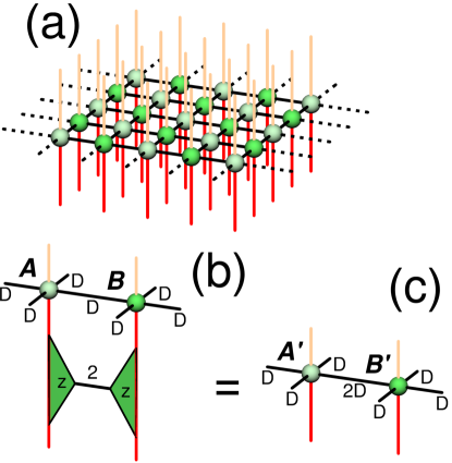
Figure 10: In a, the infinite square lattice is divided into two sublattices with tensors $A$ (lighter green) and $B$ (darker green). In b, SVD decomposition of a NN gate is applied to every pair $A$ and $B$ of NN tensors. In c, when the tensors $A$ and $B$ are contracted with their respective $z$’s, then they become new tensors $A^{\prime}$ and $B^{\prime}$ with a doubled bond dimension $2D$ on their common NN bond. By variational optimization the iPEPS made of $A^{\prime}$ and $B^{\prime}$ is approximated by a new iPEPS made of $A^{\prime\prime}$ and $B^{\prime\prime}$ with the original bond dimension $D$.

Appendix A 2-site gates

For the sake of clarity, the main text presents a straightforward single-site version of the algorithm. In practice it is more efficient to implement the gate $U_{ZZ}(d\tau)$ as a product of two-site gates. To this end the infinite square lattice is divided into two sublattices $A$ and $B$, see Fig. 10a. On the checkerboard the gate becomes a product

$$U_{ZZ}(d\tau)=U^{a}_{0}(d\tau)U^{a}_{1}(d\tau)U^{b}_{0}(d\tau)U^{b}_{1}(d\tau).$$ (22)

Here $a$ and $b$ are the Cartesian lattice directions spanned by $e_{a}$ and $e_{b}$,

$$U^{a}_{s}(d\tau) = \prod_{mn}e^{id\tau Z_{2m+s-1,n}Z_{2m+s,n}},$$ (23)

$$U^{b}_{s}(d\tau) = \prod_{mn}e^{id\tau Z_{m,2n+s-1}Z_{m,2n+s}},$$ (24)

and $Z_{m,n}$ is an operator at a site $me_{a}+ne_{b}$.

Every NN gate in (23,24) is decomposed as in (8). Consequently, when a gate, say, $U^{a}_{0}(d\tau)$ is applied to the checkerboard $AB$-iPEPS in Fig. 10a, then every pair of tensors $A$ and $B$ at every pair of NN sites $(2m-1)e_{a}+ne_{b}$ and $2me_{a}+ne_{b}$ is applied with the NN-gate’s decomposition as in Fig. 10b. When the tensors $A$ and $B$ are fused with their respective $z$’s, they become $A^{\prime}$ and $B^{\prime}$, respectively, that are connected by an index with a bond dimension $2D$, see Fig. 10c. The action of the gate $U^{a}_{0}(d\tau)$ is completed when the $A^{\prime}B^{\prime}$-iPEPS is approximated by a (variationally optimized) new $A^{\prime\prime}B^{\prime\prime}$-iPEPS with the original bond dimension $D$ at every bond.

Apart from the opportunity to use reduced tensors in the variational optimization, the main advantage of the 2-site gates is that the enlarged bond dimension $2D$ appears only on a minority of bonds. This speeds up the CTMRG for the overlap $\langle\psi^{\prime}|\psi^{\prime\prime}\rangle$ that is the most time-consuming part of the algorithm. The decomposition into 2-site gates breaks the symmetry of the lattice. Therefore we use the efficient non-symmetric version of CTMRG Corboz et al. (2014) for checkerboard lattice.

References

- Verstraete et al. (2008) F. Verstraete, V. Murg, and J. Cirac, Advances in Physics 57, 143 (2008).
- Orús (2014) R. Orús, Annals of Physics 349, 117 (2014).
- Fannes et al. (1992) M. Fannes, B. Nachtergaele, and R. F. Werner, Communications in Mathematical Physics 144, 443 (1992).
- Verstraete and Cirac (2004) F. Verstraete and J. I. Cirac, cond-mat/0407066 (2004).
- Hastings (2007) M. B. Hastings, Journal of Statistical Mechanics: Theory and Experiment 2007, P08024 (2007).
- Schuch et al. (2008) N. Schuch, M. M. Wolf, F. Verstraete, and J. I. Cirac, Phys. Rev. Lett. 100, 030504 (2008).
- Barthel (2017) T. Barthel, arXiv:1708.09349 (2017).
- White (1992) S. R. White, Phys. Rev. Lett. 69, 2863 (1992).
- White (1993) S. R. White, Phys. Rev. B 48, 10345 (1993).
- Schollwöck (2005) U. Schollwöck, Rev. Mod. Phys. 77, 259 (2005).
- Schöllwock (2011) U. Schöllwock, Annals of Physics 326, 96 (2011).
- Molnar et al. (2015) A. Molnar, N. Schuch, F. Verstraete, and J. I. Cirac, Phys. Rev. B 91, 045138 (2015).
- Ge and Eisert (2016) Y. Ge and J. Eisert, New Journal of Physics 18, 083026 (2016).
- Pineda et al. (2010) C. Pineda, T. Barthel, and J. Eisert, Phys. Rev. A 81, 050303 (2010).
- Corboz and Vidal (2009) P. Corboz and G. Vidal, Phys. Rev. B 80, 165129 (2009).
- Barthel et al. (2009) T. Barthel, C. Pineda, and J. Eisert, Phys. Rev. A 80, 042333 (2009).
- Gu et al. (2010) Z.-C. Gu, F. Verstraete, and X.-G. Wen, arXiv:1004.2563 (2010).
- Kraus et al. (2010) C. V. Kraus, N. Schuch, F. Verstraete, and J. I. Cirac, Phys. Rev. A 81, 052338 (2010).
- Corboz et al. (2010) P. Corboz, R. Orús, B. Bauer, and G. Vidal, Phys. Rev. B 81, 165104 (2010).
- Corboz et al. (2011) P. Corboz, S. R. White, G. Vidal, and M. Troyer, Phys. Rev. B 84, 041108 (2011).
- Murg et al. (2007) V. Murg, F. Verstraete, and J. I. Cirac, Phys. Rev. A 75, 033605 (2007).
- Nishio et al. (2004) Y. Nishio, N. Maeshima, A. Gendiar, and T. Nishino, cond-mat/0401115 (2004).
- Jordan et al. (2008) J. Jordan, R. Orús, G. Vidal, F. Verstraete, and J. I. Cirac, Phys. Rev. Lett. 101, 250602 (2008).
- Jiang et al. (2008) H. C. Jiang, Z. Y. Weng, and T. Xiang, Phys. Rev. Lett. 101, 090603 (2008).
- Gu et al. (2008) Z.-C. Gu, M. Levin, and X.-G. Wen, Phys. Rev. B 78, 205116 (2008).
- Orús and Vidal (2009) R. Orús and G. Vidal, Phys. Rev. B 80, 094403 (2009).
- Matsuda et al. (2013) Y. H. Matsuda, N. Abe, S. Takeyama, H. Kageyama, P. Corboz, A. Honecker, S. R. Manmana, G. R. Foltin, K. P. Schmidt, and F. Mila, Phys. Rev. Lett. 111, 137204 (2013).
- Corboz and Mila (2014) P. Corboz and F. Mila, Phys. Rev. Lett. 112, 147203 (2014).
- Zheng et al. (2017) B.-X. Zheng, C.-M. Chung, P. Corboz, G. Ehlers, M.-P. Qin, R. M. Noack, H. Shi, S. R. White, S. Zhang, and G. K.-L. Chan, Science 358, 1155 (2017).
- Liao et al. (2017) H. J. Liao, Z. Y. Xie, J. Chen, Z. Y. Liu, H. D. Xie, R. Z. Huang, B. Normand, and T. Xiang, Phys. Rev. Lett. 118, 137202 (2017).
- Corboz (2016a) P. Corboz, Phys. Rev. B 94, 035133 (2016a).
- Vanderstraeten et al. (2016) L. Vanderstraeten, J. Haegeman, P. Corboz, and F. Verstraete, Phys. Rev. B 94, 155123 (2016).
- Fishman et al. (2017) M. Fishman, L. Vanderstraeten, V. Zauner-Stauber, J. Haegeman, and F. Verstraete, arXiv:1711.05881 (2017).
- Xie et al. (2017) Z. Y. Xie, H. J. Liao, R. Z. Huang, H. D. Xie, J. Chen, Z. Y. Liu, and T. Xiang, Phys. Rev. B 96, 045128 (2017).
- Czarnik et al. (2016a) P. Czarnik, M. M. Rams, and J. Dziarmaga, Phys. Rev. B 94, 235142 (2016a).
- Corboz (2016b) P. Corboz, Phys. Rev. B 93, 045116 (2016b).
- Corboz et al. (2018) P. Corboz, P. Czarnik, G. Kapteijns, and L. Tagliacozzo, arXiv:1803.08445 (2018).
- Rader and Läuchli (2018) M. Rader and A. M. Läuchli, arXiv:1803.08566 (2018).
- Rams et al. (2018) M. M. Rams, P. Czarnik, and Ł. Cincio, arXiv:1801.08554 (2018).
- Czarnik et al. (2012) P. Czarnik, L. Cincio, and J. Dziarmaga, Phys. Rev. B 86, 245101 (2012).
- Czarnik and Dziarmaga (2014) P. Czarnik and J. Dziarmaga, Phys. Rev. B 90, 035144 (2014).
- Czarnik and Dziarmaga (2015a) P. Czarnik and J. Dziarmaga, Phys. Rev. B 92, 035120 (2015a).
- Czarnik et al. (2016b) P. Czarnik, J. Dziarmaga, and A. M. Oleś, Phys. Rev. B 93, 184410 (2016b).
- Czarnik and Dziarmaga (2015b) P. Czarnik and J. Dziarmaga, Phys. Rev. B 92, 035152 (2015b).
- Czarnik et al. (2017) P. Czarnik, J. Dziarmaga, and A. M. Oleś, Phys. Rev. B 96, 014420 (2017).
- Dai et al. (2017) Y.-W. Dai, Q.-Q. Shi, S. Y. Cho, M. T. Batchelor, and H.-Q. Zhou, Phys. Rev. B 95, 214409 (2017).
- Kshetrimayum et al. (2017) A. Kshetrimayum, H. Weimer, and R. Orús, Nature Communications 8, 1291 (2017).
- Vanderstraeten et al. (2015) L. Vanderstraeten, M. Mariën, F. Verstraete, and J. Haegeman, Phys. Rev. B 92, 201111 (2015).
- Bruognolo et al. (2017) B. Bruognolo, Z. Zhu, S. R. White, and E. M. Stoudenmire, arXiv:1705.05578 (2017).
- Chen et al. (2018) B.-B. Chen, L. Chen, Z. Chen, W. Li, and A. Weichselbaum, arXiv:1801.00142 (2018).
- Li et al. (2011) W. Li, S.-J. Ran, S.-S. Gong, Y. Zhao, B. Xi, F. Ye, and G. Su, Phys. Rev. Lett. 106, 127202 (2011).
- Xie et al. (2012) Z. Y. Xie, J. Chen, M. P. Qin, J. W. Zhu, L. P. Yang, and T. Xiang, Phys. Rev. B 86, 045139 (2012).
- Ran et al. (2012) S.-J. Ran, W. Li, B. Xi, Z. Zhang, and G. Su, Phys. Rev. B 86, 134429 (2012).
- Ran et al. (2013) S.-J. Ran, B. Xi, T. Liu, and G. Su, Phys. Rev. B 88, 064407 (2013).
- Ran et al. (2018) S.-J. Ran, W. Li, S.-S. Gong, A. Weichselbaum, J. von Delft, and G. Su, Phys. Rev. B 97, 075146 (2018).
- Peng et al. (2017) C. Peng, S.-J. Ran, T. Liu, X. Chen, and G. Su, Phys. Rev. B 95, 075140 (2017).
- Chen et al. (2017) X. Chen, S.-J. Ran, T. Liu, C. Peng, Y.-Z. Huang, and G. Su, arXiv:1711.01001 (2017).
- Vidal (2007) G. Vidal, Phys. Rev. Lett. 99, 220405 (2007).
- Vidal (2008) G. Vidal, Phys. Rev. Lett. 101, 110501 (2008).
- Evenbly and Vidal (2014a) G. Evenbly and G. Vidal, Phys. Rev. Lett. 112, 220502 (2014a).
- Evenbly and Vidal (2014b) G. Evenbly and G. Vidal, Phys. Rev. B 89, 235113 (2014b).
- Trotter (1959) H. F. Trotter, Proc. Amer. Math. Soc. 10, 545 (1959).
- Suzuki (1966) M. Suzuki, Journal of the Physical Society of Japan 21, 2274 (1966).
- Suzuki (1976) M. Suzuki, Progress of Theoretical Physics 56, 1454 (1976).
- Baxter (1978) R. J. Baxter, Journal of Statistical Physics 19, 461 (1978).
- Nishino and Okunishi (1996) T. Nishino and K. Okunishi, Journal of the Physical Society of Japan 65, 891 (1996).
- Corboz et al. (2014) P. Corboz, T. M. Rice, and M. Troyer, Phys. Rev. Lett. 113, 046402 (2014).
- Jahromi et al. (2018) S. S. Jahromi, R. Orús, M. Kargarian, and A. Langari, Phys. Rev. B 97, 115161 (2018).
- Halimeh and Zauner-Stauber (2017) J. C. Halimeh and V. Zauner-Stauber, Phys. Rev. B 96, 134427 (2017).
- Cincio et al. (2007) L. Cincio, J. Dziarmaga, M. M. Rams, and W. H. Zurek, Phys. Rev. A 75, 052321 (2007).
- Wahl et al. (2017) T. B. Wahl, A. Pal, and S. H. Simon, arXiv:1711.02678 (2017).
- Werner et al. (2016) A. H. Werner, D. Jaschke, P. Silvi, M. Kliesch, T. Calarco, J. Eisert, and S. Montangero, Phys. Rev. Lett. 116, 237201 (2016).
- Wolf et al. (2008) M. M. Wolf, F. Verstraete, M. B. Hastings, and J. I. Cirac, Phys. Rev. Lett. 100, 070502 (2008).
- Blöte and Deng (2002) H. W. J. Blöte and Y. Deng, Phys. Rev. E 66, 066110 (2002).
- Nishino et al. (2001) T. Nishino, Y. Hieida, K. Okunishi, N. Maeshima, Y. Akutsu, and A. Gendiar, Progress of Theoretical Physics 105, 409 (2001).
- Gendiar et al. (2003) A. Gendiar, N. Maeshima, and T. Nishino, Progress of Theoretical Physics 110, 691 (2003).
- Baxter (1982) R. J. Baxter, Exactly solved models in statistical mechanics (1982).
- ban Chan (2012) Y. ban Chan, Journal of Physics A: Mathematical and Theoretical 45, 085001 (2012).
- ban Chan (2013) Y. ban Chan, Journal of Physics A: Mathematical and Theoretical 46, 125009 (2013).
- Hesselmann and Wessel (2016) S. Hesselmann and S. Wessel, Phys. Rev. B 93, 155157 (2016).
- Pfeifer et al. (2014) R. N. C. Pfeifer, G. Evenbly, S. Singh, and G. Vidal, arXiv:1402.0939 (2014).