Cascade of transitions in molecular information theory

Abstract

Biological organisms are open, adaptve systems that can respond to changes in environment in specific ways. Adaptation and response can be posed as an optimization problem, with a tradeoff between the benefit obtained from a response and the cost of producing environment-specific responses. Using recent results in stochastic thermodynamics, we formulate the cost as the mutual information between the environment and the stochastic response. The problem of designing an optimally performing network now reduces to a problem in rate distortion theory – a branch of information theory that deals with lossy data compression. We find that as the cost of unit information goes down, the system undergoes a sequence of transitions, corresponding to the recruitment of an increasing number of responses, thus improving response specificity as well as the net payoff. We derive formal equations for the transition points and exactly solve them for special cases. The first transition point, also called the coding transition, demarcates the boundary between a passive response and an active decision-making by the system. We study this transition point in detail, and derive three classes of asymptotic behavior, corresponding to the three limiting distributions of the statistics of extreme values. Our work points to the necessity of a union between information theory and the theory of adaptive biomolecular networks, in particular metabolic networks.

I Introduction

Biological systems are distinctive in their ability to adaptively respond to different environments. This applies not only to organisms, but even individual cells in multicellular organismsalberts . Adaptive behavior contains the notion of specificity, i.e. the response is tailored towards the particular stimulus specificity1 ; specificity2 ; bialek . The response results in a benefit to the cell. For example, the synthesis of enzymes specific to the breakdown of a particular nutrient in the environment leads to a free-energy gain for the cell. The net free-energy payoff should however include, apart from this gain, the free-energy cost of response specificity. An optimal adaptive network evolves to maximize the difference between the benefit and the specificity cost. The degree of specificity in this biological context has been hard to quantify; part of the reason is that specificity is not the property of particular pathways, but of the entire repertoire of possible cellular responses and their regulatory mechanisms. Recent developments in information thermodynamics parrondo allow us to build a coarse-grained model of specificity cost in a system.

We model the adaptive response as a problem in coding or data compression. Consider the schematic in Figure 1. The environment comprises of a diversity of states indexed by $\alpha$, and they are presented to the cell with frequencies $f_{\alpha}$. The cell produces a response $i$ with probability $p(i|\alpha)$. In information theoretic terms, the environment state $\alpha$ is the signal and the response $i$ is the code or the representation, and the mapping $p(i|\alpha)$ is a random code. The stochastic response to the environment models the fact that responses at the cellular level are inherently noisy. From a bio-chemical perspective, the adaptive response essentially involves a transfer of information from one set of molecules to another. For example, many bacteria such as E. coli can grow on a wide variety of sugars alon . The concentration of various enzymes in a bacterial cell contains information about the nutrients in its growth medium bialek .

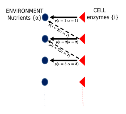
Figure 1: A cell (organism) must respond adaptively to different environmental states. The environment comprises a diversity of nutrients that occur with frequency $f_{\alpha}$ ($\alpha=1,\dots,n$). The cell responds to the environment with response probabilities $p(i|\alpha)$, where $i$ labels the cellular response. Adaptive behavior is seen as a communication channel between environment and response.

Since the environmental states occur with frequency $f_{\alpha}$, the the joint distribution of the environment state $\alpha$ and the response $i$ is given by $P(i,\alpha)=p(i|\alpha)f_{\alpha}$. The mutual information between the environment $\alpha$ and reponse $i$ is given by

$$I = \sum_{\alpha}f_{\alpha}\sum_{i}p(i|\alpha)\log\frac{P(i,\alpha)}{p(i)f(\alpha)},$$

$$= \sum_{\alpha}f_{\alpha}\sum_{i}p(i|\alpha)\log\frac{p(i|\alpha)}{p(i)},$$

where $p(i)=\sum_{\alpha}P(i,\alpha)$ is the marginal distribution of the response. The mutual information $I$ denotes the average number of nats about the environment state $\alpha$ learned from observing the response $i$. Thus, the mutual information is high when the residual uncertainty in the environment state $\alpha$ is low after observing the response $i$, i.e. the response is very specific to each environment state.

We assume here that when the environment states change to a new randomly chosen state, the adaptive response of the system is instantaneous, and the memory of the previous response is erased. This dynamics occurs on a scale much faster than adaptive evolution over fitness landscapes. Recent results in information thermodynamics have established that the minimum free energy consumed in such measurement and erasure processes is proportional to the mutual information $I$ parrondo ; tlusty_07 ; sgm . Thus, the cost of specificity is proportional to $I$. This cost is of fundamental thermodynamic origin, connected to problems involving the Maxwell’s demon parrondo , and it is also irreducible, so that it cannot be circumvented by better system design. Here we ignore the cost of producing the response machinery, but focus only on the operational cost of regulating the machinery to produce the appropriate response. Note that mutual information is a lower bound for this cost; the precise value of the free energy cost depends on the specifics of the system, and may, in general, be significantly greater than this lower bound. Nevertheless, what we lose in sacrificing some of the biological realism, we gain in the generality and tractability of the model. This allows us to identify qualitative regimes of behavior even in the absence of detailed data.

Having identified the cost of specificity, we can understand the performance of an adaptive system as involving a tradeoff between benefit and cost. We ask what an optimal response distribution, $p(i|\alpha)$, looks like, given the abundances of various environmental states. We investigate this question by deriving the general features of these distributions. Our main focus will be on biological systems that perform energy catabolism, because in these systems it is the free energy cost that is of primary relevance in analyzing system performance. In other systems, such as those involving the synthesis of proteins through transcription and translation, it is not obvious how to construct a simple qunatitative indicator of performance, and one should investigate whether the free energy cost is indeed an important limiting factor. Nonetheless, the information theoretic approach has been suggested as relevant for the origin of molecular codes in a variety of contexts tlusty_07 ; tlusty_iop . In the next section, we state our model for energy catabolism formallly as an optimization problem.

II Model

Consider an organism that is exposed to $n$ different nutrients indexed by $\alpha$, that occur in the environment with probability $f_{\alpha}$. The organism on sensing environment $\alpha$ produces a response (i.e. the synthesis of the appropriate transporters, enzymes, etc.) indexed by $i$ with a probability $p(i|\alpha)$. Let $E_{i\alpha}\geq 0$ denote the free-energy benefit to the organism from response $i$ in environment $\alpha$. The average free energy benefit is given by

$$G=\sum_{i}\sum_{\alpha}f_{\alpha}p(i|\alpha)E_{i\alpha}.$$ (1)

The free energy cost of sensing the environment and producing a particular response, i.e. coding for the environment, is proportional to the mutual information parrondo ; tlusty_07 ; sgm ; tlusty_iop . The net free energy payoff is therefore

$$F=G(p)-\kappa^{-1}I(p),$$ (2)

where the constant $\kappa$ is determined by general thermodynamic and chemical parameters that are independent of the channel. A higher $\kappa$ is associated with a lower cost of specificity.

An optimal metabolic network would tune the channel $p(\cdot|\cdot)$ to maximize the payoff $F$, i.e. solve the optimization problem

$$\mbox{max}_{p(\cdot,\cdot)}\ G-\kappa^{-1}\ I(p).$$ (3)

Note that this problem is equivalent to the problem

$$\mbox{min}_{p(\cdot,\cdot)}\ -\kappa\sum_{i}\sum_{\alpha}f_{\alpha}p(i|\alpha)E_{i\alpha}+I(p),$$ (4)

i.e. a rate distortion problem with the distortion function $d(i,\alpha)=-E_{i\alpha}$ cover . The distortion function is a loss term that measures the performance of the code, wheareas $I$ is the quantity of information with which to minimize the loss. In our interpretation, the first term in (3) is a benefit term that depends on the specificity of the molecular code, wheareas the fidelity incurs a cost given by the second term.

This formulation is not limited to metabolic responses. It should be applicable wherever the free energy cost is relevant, and the benefit is linear in the conditional probabilities. For example, rate distortion theory has been used to investigate the origins of the genetic code in tlusty_07 .

As a generic example of how the optimal solution behaves, we numerically compute in Figure 2 the mutual information and conditional probabilities for a particular parameter set when $n=6$, as a function of $\kappa$. The data are generated by calculating the optimal channel by an alternating minimization procedure called the Blahut-Arimoto algorithm cover . The procedure is described in Appendix A. The notable feature of the plot is that the mutual information $I$ is $0$ at $\kappa=0$, and $I$ undergoes a sequence of bifurcations as $\kappa$ increases, analogous to continuous transitions in thermodynamic systems. The first bifurcation point has been called the coding transition in a related context tlusty_iop – this is the value of $\kappa$ subsequent to which the mutual information becomes non-zero. Each transition point is characterized by the fact that a new response is “switched on”. For example, in Figure 2, the response probability $p(2)$ becomes non-zero at the coding transition point. As $\kappa$ increases, we see a sequence of such transitions, where typically only one response is activated at a time. We call this sequence of transitions a cascade. Similar cascades have been observed previously at the interface of statistical mechanics and computer science, such as in the application of deterministic annealing to clustering, classification and other computational problems rose . The following section finds analytical solutions for the cascades.

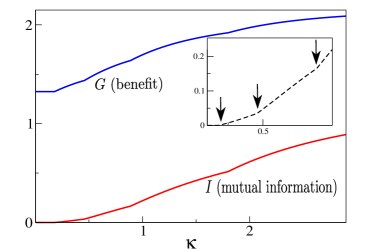
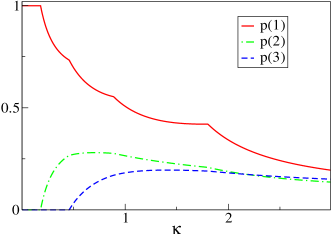
Figure 2: Cascade of transitions with $n=6$. Parameters: $E_{\alpha,\alpha}=\alpha+0.2$, $f_{\alpha}\sim 6/(\alpha-0.4)$, $E(i,j)=0.2E(i,i)$, for $j\neq i$. (Upper panel) The benefit and mutual information as a function of $\kappa$ are plotted. The inset 2 zooms in on the first three transition points, marked by arrows. (Lower panel) The first three responses to be turned on. The response $p(1)$ is the optimal non-coding response; $p(2)$ is turned on at the first transition point, also called the coding transition.

III Analysis of cascades

When $\kappa=0$, the cost of unit information is infinite, therefore the mutual information $I=0$. Thus, the response $p(i|\alpha)$ is, in fact, independent of the environment, i.e. $p(i|\alpha)=p(i)$. Since $I(p)=0$, the optimization problem reduces to

$$\max_{p}\ \sum_{i}p(i)\Big{(}\sum_{\alpha}f_{\alpha}E_{i\alpha}\Big{)}.$$

It is clear that the optimal $p^{\ast}(i)=\delta_{ir}$, where $r=\text{argmax}\{\sum_{\alpha}f_{\alpha}E_{i\alpha}\}$. Thus, the organism uses the response $r$ irrespective of the environment state $\alpha$. We will refer to $r$ as the optimal non-coding response.

As $\kappa$ increases, at some point the mutual information becomes non-zero, i.e. the response $p(i|\alpha)$ does depend on $\alpha$. This is called a coding transition in a related context tlusty_iop because the organism senses and codes the environment in terms of the response. As $\kappa$ continues to increase, we see more and more responses being activated, each accompanied by a kink in the mutual information and the benefit $G$ (see Figure 2). In the simplest interpretation, each response represents the expression of a particular gene (or operon). The task of regulating the expression is carried out by transcription factors in the cells, and the free energy cost associated with the specificity of the responses arises out of the activity of the regulatory machinery. The existence of cascades tells us that in an optimal metabolic network, a particular metabolic response may not be expressed even when the appropriate enzyme-coding genes and the corresponding nutrients are present in the system. The number of responses available from an optimal metabolic network is limited by the unit cost of information.

The distinctive feature of the cascades is that the responses are activated one at a time. It is not clear a priori that it should be so. One may think naively that for any $\kappa>0$, all responses would be active; or that, in general, multiple responses should be switched on at a transition point. We demonstrate in the following subsection that cascades are indeed generic.

III.1 Cascades are generic

We show below that under generic choice of parameters, two different responses cannot transition at the same $\kappa$. We start by assuming that the vector of free-energy $E_{i}=\{E_{i\alpha}\}_{\alpha=1}^{n}$ corresponding to response $i$ are distributed according to a distribution that has an $n$-dimensional density. Thus, $\mathbb{P}(E_{i}\in A)=0$ for any set $A$ that has dimension at most $(n-1)$.

Let $p(i)=\sum_{\alpha}p(i|\alpha)f_{\alpha}$ denote the marginal probability for response $i$. For $\kappa>0$, results in Chapter 10 of cover establish that $p$ is optimal, if and only if,

$$\sum_{\alpha}\frac{f_{\alpha}e^{\kappa E_{i\alpha}}}{\sum_{j}p(j)e^{\kappa E_{j\alpha}}}\left\{\begin{aligned} \leq 1&&p(i)=0,\\ =1&&p(i)>0.\end{aligned}\right.$$ (5)

Strong convexity of mutual information implies that the optimal solution $p_{\kappa}$ is unique and a continuous function of $\kappa$. The optimal solution for $\kappa=0$ can be obtained by taking the limit of $\kappa\searrow 0$.

Now, fix a response index $s$. We call $\kappa_{s}$ a transition point for the response $s$ if $p_{\kappa_{s}}(s)=0$ and there exists $\epsilon_{s}>0$ such that $p_{\kappa}(s)>0$ for all $\kappa\in(\kappa_{s},\kappa_{s}+\epsilon_{s}]$. By the continuity property it follows that

$$\sum_{\alpha}\frac{f_{\alpha}e^{\kappa_{s}E_{s\alpha}}}{J_{\kappa_{s}}(\alpha)}=1$$

where $J_{\kappa}(\alpha)=\sum_{j}p_{\kappa}(j)e^{\kappa E_{j\alpha}}$.

Suppose $\kappa_{s}$ is a transition point for another index $t\neq s$, i.e. $p_{\kappa_{s}}(t)=0$ and there exists an $\epsilon_{t}>0$ such that $p_{\kappa}(t)>0$ for all $\kappa\in(\kappa_{s},\kappa_{s}+\epsilon_{t}]$. Thus, a necessary condition is that

$$\sum_{\alpha}\frac{f_{\alpha}e^{\kappa_{s}E_{t\alpha}}}{J_{\kappa_{s}}(\alpha)}=1.$$

Note that $p_{\kappa_{s}}(t)=0$ implies that $E_{t}=\{E_{t\alpha}\}_{\alpha=1}^{n}$ is not included in the sum defining $\{J_{\kappa_{s}}(\alpha)\}_{\alpha=1}^{n}$. Therefore,

$$\mathbb{P}\big{(}\text{$\kappa_{s}$ is a transition point for $t$}\big{)}$$

$$\leq \mathbb{P}\left(\sum_{\alpha}\frac{f_{\alpha}e^{\kappa_{s}E_{t\alpha}}}{J_{\kappa_{s}}(\alpha)}=1\right)=0,$$

where the last equality follows from the fact that the probability that $E_{t}$ lies in an $(n-1)$ dimensional hyperplane is zero, which follows from our starting assumption. (We reiterate that the case of $\kappa=0$ has to be analysed as a limit, in which case the same conclusions will follow.)

III.2 Structure of bifurcation points for diagonal response

Starting in this section we will focus on the special case where the benefits are diagonal, i.e $E_{i\alpha}=E_{\alpha}\delta_{i\alpha}$. This is a reasonable approximation in the context of metabolic responses, since enzymes are generally highly specific to substrates. In this section, we focus on computing the bifurcation points $\kappa$.

Define $g_{\alpha}=f_{\alpha}E_{\alpha}$. Then, the object to be maximized is

$$\mathcal{L}=G-\kappa^{-1}I+\sum_{\alpha}\lambda_{\alpha}\sum_{i}p(i|\alpha),$$

where the last term, involving the set of Lagrange multipliers $\lambda_{\alpha}$, ensure the normalization of the response probabilities. Equating the derivative of this to zero, we have

$$p(i|\alpha)=p(i)\exp[\kappa(\frac{\lambda_{\alpha}}{f_{\alpha}}+\frac{g_{i}}{f_{i}}\delta_{i,\alpha})].$$ (6)

Solving for $\lambda_{\alpha}$ and substituting the result, we obtain the relations:

$$p(i|\alpha) = \frac{p(i)e^{\kappa E_{i}\delta_{i\alpha}}}{1+p(\alpha)(e^{\kappa E_{\alpha}}-1)}$$ (7)

We use the relation $p(i)=\sum_{\alpha}p(i|\alpha)f_{\alpha}$ in conjunction with the above equations to obtain

$$\sum\limits_{\alpha\neq i}\frac{f_{\alpha}}{1+p(\alpha)(e^{\kappa E_{\alpha}}-1)}+\frac{f_{i}e^{\kappa E_{i}}}{1+p(i)(e^{\kappa E_{i}}-1)}=1,$$

for $p(i)>0$.

The sum can be rewritten as

$$\sum\limits_{\alpha}\frac{f_{\alpha}}{1+p(\alpha)(e^{\kappa E_{\alpha}}-1)}+\frac{f_{i}(e^{\kappa E_{i}}-1)}{1+p(i)(e^{\kappa E_{i}}-1)}=1$$

Define $C=\sum\limits_{\alpha}\frac{f_{\alpha}}{1+p(\alpha)(e^{\kappa E_{\alpha}}-1)}$. Then, from the above equation,

$$p(i)=\frac{f_{i}}{1-C}-\frac{1}{e^{\kappa E_{i}}-1}.$$ (8)

Thus, it follows that

$$p(i)>0\quad\Leftrightarrow\quad h_{i}(\kappa):=f_{i}(e^{\kappa E_{i}}-1)>1-C.$$ (9)

Let us define the active set as $A=\{i:p(i)>0\}$. Then substituting (8) in the definition of $C$, we get that

$$C=(1-C)\sum\limits_{i\in A}\frac{1}{e^{\kappa E_{i}}-1}+\sum\limits_{j\notin A}f_{j},$$

Substituting the solution for $C$ in (8) we obtain that for all $i\in A$,

$$p(i)=\frac{f_{i}}{\sum\limits_{m\in A}f_{m}}\big{(}1+\sum\limits_{j\in A}\frac{1}{e^{\kappa E_{j}}-1}\big{)}-\frac{1}{e^{\kappa{E_{i}}}-1}.$$ (10)

This does not specify the solution for the marginals of the response probability completely, since we still need to know the active set $A$. We need to understand how the active set changes as $\kappa$ increases. At $\kappa=0$, the only member of the active set is the optimal non-coding response. As $\kappa$ increases, we expect the size of the active set to increase. However, it is also possible for responses to exit the active set; see Figure 3 for such an example. Such cases make the composition of the active set difficult to track and the the bifurcation points harder to determine. Below we find conditions under which the behavior of the active set is more regular, and use it to find the bifurcation points analytically.

First, we fix $\kappa$ and reorder the indices such that $h_{i}(\kappa)\geq h_{j}(\kappa)$ for $i\leq j$. Then (9) implies that the active set $A=\{i:i\leq\ell\}$, i.e. we only need to search over $\ell$. The index $\ell$ is optimal for $\kappa$ if $p_{i}>0$ for all $i\leq\ell$, and $p_{i}=0$ for $i>l$.

Next, we characterize special cases where there exist thresholds $\{\kappa_{i}:1\leq i\leq n\}$ such that $p(i)>0$ for all $\kappa>\kappa_{i}$. In other words, no response exits the active set as $\kappa$ increases, and the cascade consists entirely of transitions into the active set.

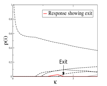
Figure 3: Here we show a simulation of the optimal marginal probabilities $p(i)$, for $n=40$; the diagonal benefit values $E_{ii}$ were chosen randomly from a uniform distribution, whereas the off-diagonal $E_{i\alpha}$ were chosen uniformly from $[0,\sigma_{od}E_{i,i}]$, with $\sigma_{od}=0.9$. The red curve shows a response that is switched on at a particular value of $\kappa$ and exits the active set at a higher value of $\kappa$. Some of the other responses that do not exit the active set are shown in dashed lines for comparison. As $\sigma_{od}$ decreases, instances of exits from the active set become rare.

Lemma 1

Suppose either (a) $E_{i}\equiv E$ or (b) $f_{i}\equiv f=\frac{1}{n}$. Then there exists thresholds $\kappa_{m}$ such that $p(m)>0$ for all $\kappa>\kappa_{m}$.

From (9) it follows that in both the special cases (a) and (b), the ordering $\{h_{i}(\kappa):1\leq i\leq n\}$ is independent of $\kappa$. Order the indices $i$ such that $h_{i}(\kappa)\geq h_{j}(\kappa)$ for all $i<j$. From (10), it follows that $p(m)>0$ if, and only if,

$$\sum_{j\leq m}f_{j}\left(\frac{1}{h_{i}(\kappa)}-\frac{1}{h_{j}(\kappa)}\right)<1$$

Define $\Delta_{i}(\kappa)=\frac{1}{h_{i+1}(\kappa)}-\frac{1}{h_{i}(\kappa)}$ for $i<n$. We show that in both cases (a) and (b), $\Delta_{i}(\kappa)=\frac{1}{h_{i+1}(\kappa)}-\frac{1}{h_{i}(\kappa)}$ which is clearly monotonically decreases with $\kappa$. Define $\kappa_{m}$ to be the solution of the equation

$$\sum_{j\leq m}f_{j}\left(\frac{1}{h_{i}(\kappa)}-\frac{1}{h_{j}(\kappa)}\right)\\ =\sum_{j<m}\big{(}\sum_{k\leq j}f_{k}\big{)}\Delta_{j}(\kappa)=1.$$

Then the monotonicity of $\Delta_{j}(\kappa)$ implies that $p(m)~{}=~{}0$ for all $\kappa\leq\kappa_{m}$ and $p(m)>0$ for all $\kappa>\kappa_{m}$.

For case (a)

$$\Delta_{i}(\kappa)=\left(\frac{1}{f_{i+1}}-\frac{1}{f_{i}}\right)(e^{\kappa E}-1)^{-1},$$

and clearly monotonically decreasing in $\kappa$. Define $x={(e^{\kappa_{m}E}-1)}^{-1}$, and $F_{m}=\sum_{j\leq m}f_{j}$. From (9) we have

$$\frac{f_{m}}{F_{m}}(1+mx)-x=0.$$

Thus,

$$\kappa_{m}=\frac{1}{E}\ln\left(\frac{F_{m}}{f_{m}}-(m-1)\right).$$

The organism transitions to a coding mode when at least two responses have a positive probability of occurring. This transition occurs at

$$\kappa_{2}=\ln(\frac{f_{1}}{f_{2}}).$$

Thus, the coding transition point depends rather weakly on the ratio of highest to second highest frequencies. Let us treat some particular instances of this case. Consider exponentially decreasing frequencies of the form $f_{m}\sim 2^{-c_{n}m}$, where $c_{n}$ is some constant that, in general, depends on the total number of nutrients $n$. The solution for the transition points is:

$$\kappa_{m}=\ln\big{[}\frac{2^{c_{n}}(2^{c_{n}m}-1)}{2^{c_{n}}-1}-(m-1)\big{]}$$

Consider the case where $c_{n}=1$. Then,

$$\kappa_{m}=\ln(2^{m}-m).$$

At large $m$, the transition point $k_{m}$ is linear in $m$, although the frequencies decay exponentially in $m$. Thus, the information cost need not be very low for the responses to rare nutrients to be active. This feature can be generically expected because of the logarithmic dependence of the transition point on $\frac{F_{m}}{f_{m}}$. A numerical verification of the result above is given in Figure5a.The fact that $\kappa_{m}$ is independent of $n$ is somewhat counterintuitive, since we would expect the transitions to occur earlier when the diversity is larger. This would occur if we choose a $c_{n}$ that goes to zero asymptotically, in which case, for large $n$,

$$\kappa_{m}\approx\frac{c_{n}}{2}(m-1).$$

In particular, if $c_{n}=\frac{1}{n}$, then $\kappa_{m}\approx\frac{m-1}{2n}$, so the transition points are inversely proportional to the diversity $n$. The crucial diffetrence between the two cases is that in the former, the ratio of the frequencies are independent of $n$, whereas in the latter case, the different frequencies start to crowd together, i.e the ratio of any two frequencies $f_{l}$ and $f_{m}$ approach $1$ in the limit of large $n$.

For case (b), the derivative

$$\Delta_{i}^{\prime}(\kappa)=\frac{E_{i}e^{\kappa E_{i}}}{f(e^{\kappa E_{i}}-1)^{2}}-\frac{E_{i+1}e^{\kappa E_{i+1}}}{f(e^{\kappa E_{i+1}}-1)^{2}}$$

Define $\alpha=\frac{E_{i}}{E_{i+1}}>1$ and $x=e^{\kappa E_{i+1}}>1$. Then

$$\Delta_{i}^{\prime}(\kappa)=\frac{\alpha x^{\alpha}}{f(x^{\alpha}-1)^{2}}-\frac{x}{f(x-1)^{2}}.$$

Fix $x>1$, and define $g(\alpha)=\frac{\alpha x^{\alpha}}{(x^{\alpha}-1)^{2}}$. Then

$$g^{\prime}(\alpha)=\frac{x^{\alpha}W(\alpha\ln(x))}{(x^{\alpha}-1)^{3}}$$

where $W(y)=e^{y}(1-y)-(1+y)$ for $y\geq 0$. Since $x>1$ and $\alpha>1$, the sign of $g^{\prime}(\alpha)$ is the same as that of $W$. We see that $W(0)=0$, and $\frac{dW}{dy}=-(ye^{y}+1)<0$ for all $y$. Therefore $W(y)<0$ for $y>0$; consequently, $g^{\prime}(\alpha)<0$ and $\Delta_{i}(\kappa)^{\prime}=\frac{1}{f}\big{(}g(\alpha)-g(1)\big{)}<0$, i.e. $\Delta_{i}(\kappa)$ is monotonically decreasing.

Figure 4: The fraction of cases where at least one exit from the active set happens as $\kappa$ increases from $0$. The diagonal benefit values $E_{ii}$ and the unnormalized frequencies are chosen uniformly from $[0.5,1.5]$. The off-diagonal benefit values $E_{ij}$ are chosen uniformly from $[0,\sigma_{od}E_{ii}]$. When $\sigma_{od}$ is less than $0.5$, exits become extremely rare, and typically no exits are found in a set of $10^{3}$ different realizations.

In this case, one cannot solve for the bifurcation points $\kappa_{m}$ exactly. However, one can approximate $\kappa_{m}$ when $\kappa_{m}E_{i}\ll 1$ for all $i\leq m$. We can then expand (10) up to linear order in $\kappa E_{i}$ and obtain the solution

$$\kappa_{m}\approx\frac{m}{E_{m}}-\sum_{j=1}^{m}\frac{1}{E_{j}}.$$

See Figure5b for comparison of the prediction with data. Unlike in Case (a), the bifurcation points depend more sensitively on the benefit values $E_{i}$. Once again, consider the coding transition point, $\kappa_{2}$. If $E_{2}\ll E_{1}$, it can be shown that $\kappa_{2}\approx\ln(2)(\frac{E_{1}}{E_{2}})$, i.e the coding transition depends linearly rather than logarithmically on the ratio of highest to second-highest benefits. In an approximate sense, a low-frequency nutrient is more likely to be coded for than a low-benefit nutrient.

In general, the bifurcation points can be solved for when the ordering of the $h_{i}$ are independent of $\kappa$. This happens when $f_{i}\leq f_{j}$ if and only if $E_{i}\leq E_{j}$ for all $i,j$. When this condition is violated, the ordering depends on $\kappa$, and the active set becomes harder to identify. When one also allows for the off-diagonal elememts $E_{i\alpha}$ to be non-zero, we find numerically that exits from the active set do happen. It is shown in Figure 4 that exits are common when the off-diagonal terms are large, but as they become smaller, exits become very rare and eventually cannot be numerically detected at all.

The optimal $p(i|\alpha)$ for $\alpha\neq i$ satisfies

$$\frac{p(i|\alpha)}{p(i)}=\frac{1}{1+p(\alpha)(e^{\kappa E_{\alpha}}-1)}<p(\alpha|\alpha)$$ (11)

This makes intuitive sense, since the off-diagonal responses do not contribute to the benefit term. Note that the off-diagonal $p(i|\alpha)$ is positive whenever a response is active, i.e. $p(i)>0$. In an experimental context, such non-cognate responses may show up merely as noise, but our analysis here indicates that it may be the result of an optimization process. Although the off-diagonal terms do not increase the benefit, they contribute to decreasing the mutual information, and therefore increase the net payoff. Third, when the response $\alpha$ is not active, we have $p(i|\alpha)=p(i)$, i.e the metabolic response contains no information about the nutrients in the non-active set.

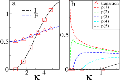
Figure 5: a. Mutual information and net payoff for an exactly solvable case, with $E_{m}=1$, and $f_{m}=\frac{2^{-m}}{1-2^{-n}}$, for $n=7$. The dashed lines are from the numerically obatined solutions, whereas the symbols are the exact solutions at the transition point. b. The approximate transition points for the case $f_{i}=1/n$, $E_{\alpha}=1-(\alpha-1)^{2}/n^{2}$, for $n=8$, are marked as triangles. They are compared with the numerically obtained transition points for the second to fifth responses. The approximation fits the data well up to the third transition point.

Among all the transition points, the coding transition is special because it separates the regime of constant response from a regime where the organism must sense the environment. We devote the next section to the analysis of the coding transition, i.e. the value $\kappa^{\ast}$ when the conditional distribution $p(i|\alpha)$ is no longer uniform for all environment states $\alpha$.

IV Asymptotics of the Coding Transition and the theory of extreme values

The coding transition has been suggested as the origin of molecular codes in biology tlusty_iop . Here we ask the question: how generic is the phenomenon of metabolic coding? When the number of nutrients is small, $\kappa^{\ast}$ has a finite value, but as the number of nutrients increases, there is an increasing benefit to be had from distinguishing the nutrients, and we could expect $\kappa^{\ast}$ to be small. But does it go to $0$ asymptotically, and if so, at what rate? We will see in the following that the answer depends on the distribution of frequencies and benefits of the nutrients, and certain universality classes of the coding behavior can be identified from the theory of extreme value statistics.

Recall that when $\kappa=0$, the optimal response is non-coding, and the optimization problem becomes:

$$\max_{p}\sum_{i}p(i)g_{i},$$

where $g_{i}=f_{i}E_{i}$. The optimal solution is $p_{0}(i)=\delta_{ir}$, where $r=\text{argmax}\{g_{i}\}$. This solution remains optimal provided

$$\sum_{\alpha}\frac{f_{\alpha}e^{\kappa E_{i\alpha}}}{\sum_{j}p_{0}(j)e^{\kappa E_{j\alpha}}}\leq 1$$

for all $i\neq r$. For the special case where $E_{i\alpha}=E_{\alpha}\delta_{i\alpha}$, this condition reduces to

$$f_{i}e^{\kappa E_{i}}+f_{r}e^{-\kappa E_{r}}\leq f_{i}+f_{r},$$

for all $i\neq r$. Thus, the coding transition point $\kappa^{\ast}$ is smallest positive value of $\kappa$ that solves one of the $n-1$ equations

$$\frac{f_{i}}{f_{r}}(e^{\kappa E_{i}}-1)=1-e^{-\kappa E_{r}}$$

for $i\neq r$. Let $x=e^{\kappa E_{r}}$, $s_{i}=\frac{E_{i}}{E_{r}}$, and $w_{i}=\frac{f_{i}}{f_{r}}$. Then the above equation reduces to

$$w_{i}x^{1+s_{i}}=(1+w_{i})x-1.$$ (12)

One solution is $x^{\ast}=1$ corresponding to $\kappa=0$. Our goal is to compute the non-trivial solution $x^{\ast}>1$. In typical scenarios, the precise distribution of nutrient benefits $E_{\alpha}$ are unlikely to be known, and hence the precise value of $x^{\ast}$ cannot be computed. However, one may be able to identify certain universal features of the coding transition $x^{\ast}$ as a function of the distribution of benefits $\{E_{\alpha}\}_{\alpha=1}^{n}$ and the frequencies $\{f_{\alpha}\}_{\alpha=1}^{n}$. We assume that $E_{\alpha}$ are independent identically distributed samples from a fixed distribution $\pi_{E}$, and $f_{\alpha}=\frac{h_{\alpha}}{\sum_{\alpha^{\prime}}h(\alpha^{\prime})}$ where each term $h_{\alpha}$ is an independent sample from the distribution $\pi_{h}$.

We will focus on cases where the coding transition occurs at $\kappa^{\ast}\approx 0$ as $n\rightarrow\infty$, equivalently, at $x^{\ast}=1+y$, for $y\ll 1$. Substituting $y_{i}=x_{i}-1$ in (12), and expanding up to second order in $y_{i}$, we get

$$y_{i}=\frac{2(1-s_{i}w_{i})}{1-\frac{1}{2}s_{i}w_{i}(1-s_{i})},$$ (13)

which holds for all $y_{i}\ll 1$. Since $s_{i}w_{i}=\frac{f_{i}E_{i}}{f_{r}E_{r}}=\frac{g_{i}}{g_{r}}<1$, we have that $y_{i}>0$, as required. We show in the Appendix that when the distribution of $E$ is bounded, the above equation further reduces to

$$y_{i}\approx{2(1-s_{i}w_{i})},$$ (14)

and therefore the transition corresponds to the largest value of $s_{i}w_{i}$. Under this approximation, the coding transition is determined by the distribution of the product $g_{i}=f_{i}E_{i}$, and not the distributions of the individual terms $f_{i}$ and $E_{i}$. Define $\rho_{i}=g_{i}/g_{r}$, where $g_{r}$ is the benefit associated with the non-coding response. Clearly, $\rho_{i}<1$, and

$$\kappa^{\ast}=2(1-\rho),$$ (15)

where $\rho=\max_{i\neq r}\{\rho_{i}\}$. Thus, the distribution of $\kappa^{\ast}$ is determined by the distribution of $\rho$, i.e. the ratio of the second highest to highest value out of $n$ values chosen independently from an identical distribution $Q(x)$. Along the lines of Eq 13 in satya , we can write

$$P_{2}(x,x_{1})=nQ(x)P_{max}(x_{1};n-1)\Theta(x-x_{1})$$

where the term $nQ(x_{1})$ is the probability that any one of the $n$ chosen numbers has the value $x_{1}$, and $P_{max}(x;n-1)$ is the probability that among the remaining $n-1$ numbers (which were chosen independently from $Q(x)$), $x$ is the highest value; the Heaviside step function $\Theta$ ensures that the probability is zero when $x>x_{1}$. We need to characterize the ratio $\rho=x/x_{1}$ using this distribution. It is natural to split the problem into three different classes of distribution $Q$, which are known to exhibit different extreme value behavior book .

IV.1 Asymptotic classes

Suppose $n$ values $X_{i}$ are sampled independently from a distribution $Q$. Let $x_{n}=\max_{1\leq i\leq n}\{X_{i}\}$ denote the maximum of these $n$ samples. Then there exist coefficients $a_{n}$, and $b_{n}$ such that the distribution of $x_{n}$ for large $n$ is given by $b_{n}^{-1}f(\frac{x-a_{n}}{b_{n}})$, where the function $f$ is one of three universal limiting forms of extreme value statistics. The precise form the limiting distribution $f$ is determined by the tail of the parent distribution $Q$. In this section, we compute the asymptotic behavior of the value of the coding transition $\kappa^{\ast}$ for particular distrubutions belonging to each of the three canonical classes satya . We consider the classes in decreasing order of how fast the tail of the parent distribution decays.

(i) Bounded distributions Consider a bounded distribution of the form $Q(x)\sim(a-x)^{\beta-1}$, $\beta>0$ with the support $0\leq x\leq a$. This covers a broad range of asymptotic behaviors that commonly occur as $x\to a$ satya . In this case, the asymptotic distribution $f(z)$ of the scaled maximum $z=b_{n}^{-1}(x_{n}-a_{n})$ is of the Weibull form

$$f(z)\sim{(-z)}^{\beta-1}\exp\big{(}-(-z)^{\beta}\big{)}\$$

for $a_{n}=a$ and $b_{n}=n^{-1/\beta}$.

Let $x$ denote second highest value among the $n$ terms, and let $x+\epsilon$, $\epsilon>0$, denote the highest value among the $n$ terms. Then the joint distribution of $(x,\epsilon)$ is given by $nQ(x+\epsilon)P_{max}(x;n-1)$. In Appendix C, we show that this form of the joint distribution implies that the mean value of $\kappa^{\ast}=2(1-\rho)=2\langle\frac{\epsilon}{x_{n}+\epsilon}\rangle$, and in the large $n$ limit it is given by

$$\kappa^{\ast}\sim n^{-1/\beta}.$$

For a uniform distribution $\beta=1$, and $\kappa^{\ast}$ is inversely proportional to $n$. The asymptotic decay of the transition point is fastest for this class of distributions. Comparison of the result with numerical data in Figure 6a reveals an excellent match.

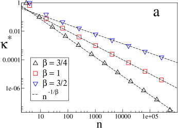
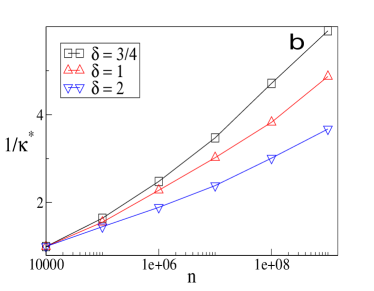
Figure 6: The scaling of the coding transition point as a function of total number of nutrients. (a) The result for bounded distribution, with the predicted scaling shown in dashed lines. The symbols represent data points obtained from numerical simulation. (b) The inverse of $\kappa^{\ast}$ plotted on log-linear scale. The curves have been normalized by the value at $n=10^{4}$ for clear visibility in a single frame. The theory predicts a linear curve; but the convergence to the asymptotic logarithmic regime is extremely slow, and only the approach to the regime can be detected in the plots.

(ii) Unbounded distributions with light tails  Next, we consider the case where the support of $Q$ is unbounded; however, the tail of $Q$ is faster than power law. We restrict ourselves to distributions of the form $Q(x)\sim\exp(-x^{\delta})$,with $\delta>0$ satya , which cover a broad class of distributions that occur in natural settings, including exponential, Gaussian and stretched exponential form stretched . In this case, the limiting distribution of the scaled maximum $z=b_{n}^{-1}(x_{n}-a_{n})$ is the Gumbel distribution of the form $f(z)=e^{-z-e^{-z}}$, and

$$a_{n} = (\ln n)^{\frac{1}{\delta}}+\frac{1}{\delta}(\frac{1}{\delta}-1)(\ln n)^{\frac{1}{\delta}-1}\ln(\ln n)$$ (16)

$$b_{n} = \frac{1}{\delta}(\ln n)^{\frac{1}{\delta}-1}.$$ (17)

Using this limiting form, and a calculation similar to the bounded case (see Appendix C for details), we get

$$\kappa^{\ast}\sim{(\ln n)}^{-1}.$$

In this case, the coding transition point goes to zero very slowly. Consequently, even in a highly nutrient diverse environment, the organism may not sense and encode the environment. Comparison with numerical simulation data is shown in Figure 6b.

(iii) Power law distributions   When $Q$ has a power law tail, we can show that $\kappa^{\ast}$ does not go to zero in the large $n$ limit. Consider $Q(x)$ of the form $Q(x)=\alpha e^{-x^{-\alpha}}x^{-(1+\alpha)}$, $\alpha>0$. In this case, the asymptotic distribution $f(z)\sim\frac{\alpha}{z^{1+\alpha}}e^{-z^{-\alpha}}$ is the Fréchet distribution, with $a_{n}=0$, and $b_{n}=n^{\frac{1}{\alpha}}$. As before, let $x$ denote the second largest value and $x+\epsilon$ denote the highest value. Then

$${\langle\frac{\epsilon}{x}\rangle} \sim \frac{n^{\frac{2}{1+\alpha}}}{\alpha-1},\mbox{~{} $\alpha>1$}$$ (18)

$$\sim \infty,\mbox{~{}~{}~{}~{}~{}~{}~{}$\alpha\leq 1$.}$$

The details of the calculation are in Appendix C. For $n\rightarrow\infty$, we see that the mean ratio of the highest to second highest values diverges, even for $\alpha>1$ (where the mean of the parent distribution is finite). We show in Appendix C that this implies $\kappa^{\ast}$ also diverges asymptotically. The heavy tails of the distributions cause the largest selected value to dominate over all other values, and thus the organism is not in the coding regime.

IV.2 Discussion

When $\kappa>\kappa^{\ast}$, the organism senses the environment, encodes information about the environment, and takes an appropriate response. Note that the response $i$ is a potentially a random map from the environment state $\alpha$. This stochastic response is, often, critical for the survival of the population. The value of $\kappa^{\ast}$ depends on the distribution of environmental states and the free benefit associated the particular response; therefore, the precise value of $\kappa^{\ast}$ cannot be precisely calculated. However, universal behavior emerges in the limit of a large number of environmental states. The behavior falls into three different classes as a function of the tail of the distributions of the environment frequency $f_{\alpha}$ and the free energy benefit $E_{\alpha}$. We show that only limiting behaviour of $\kappa^{\ast}$ is a function of the product $g_{\alpha}=f_{\alpha}E_{\alpha}$. When $g_{\alpha}$ are chosen from a bounded distribution, the mean $\kappa^{\ast}$ goes to $0$ as $n^{-1/\beta}$ as a function of the number of environment states $n$. In the case of unbounded distributions with light tails, the mean $\kappa^{\ast}$ decays to zero as $(\ln n)^{-1}$, and the mean $\kappa^{\ast}$ can diverge for power law distributions. The divergence is an artifact of the power law distribution, but what it does imply is that there is no typical $\kappa$ above which we can expect an organism to be in the coding regime. The slow convergence in the case of exponential or Gaussian tails is more surprising, since one would have expected the organism to code for the environment when the product is drawn from such distributions.

Which of these cases, if any, occur in natural environments is a difficult question to answer. We may expect that in highly biodiverse environments, such as in soil microbial communities, the number of available nutrients is high. Such communities harbor hundreds of different species of microbes, and their interactions often promote chemical diversity metabolites . A thorough quantitative study of nutrient distributions in such communities would be helpful in making predictions about the coding behavior of metabolic systems.

V Conclusion

We have formulated the problem of adaptive response in biological systems as an optimization problem where the tradeoff is between the benefit obtained from specific responses and the cost of producing them. Our main result is that there is a cascade of responses as a function of the cost of information, and the number of responses that are active in an optimal metabolic system depends on the cost and the distribution of nutrients. Even when the system is capable of producing $n$ different responses, the number of responses it actually uses can be significantly smaller.

The decision to express certain genes is executed by the regulatory machinery, and evolutionary processes may lead to machinery that produces the optimal response when supplied with a certain environment. The traditional view has been that in order to metabolize new nutrients, genotypic changes that produce new or altered enzymes are required. However, our model points to the existence of epigenetic mechanisms that carry out a decision theoretic task – that of constructing the optimal response channel from within the repertoire of responses already available. Our model is based on a particular way of looking at such regulatory mechanisms – namely that they optimal solutions of a particular in rate distortion problem.

In this paper, we only characterize the structure of the optimal channe. We do not describe how these regulatory mechanisms evolve, or indeed about the kind of molecular processes necessary to establish the optimal channel. More detailed studies are required to address these questions. Further investigations may bring out new surprises, but we believe that some of the central features of our results will continue to hold.

VI Appendix

VI.1 Algorithm for finding optimal channel

Here we consider the problem of computing the optimal $p(i|\alpha)$ for $\kappa\neq 0$. Let

$$J(p,q) = \sum_{i\alpha}f_{\alpha}p(i|\alpha)\log\left(\frac{p(i|\alpha)}{q(i)}\right)$$

$$= I(p)+D(p\|q),$$

where $D(p,q)$ denotes the relative entropy of $p$ and $q$. Then, $J(p,q)$ is jointly convex in $(p,q)$ and moreover, $\min_{q}J(p,q)=I(p)+\min_{q}D(p,q)=I(p)$. Since $G(p)-\kappa^{-1}J(p,q)$ is jointly concave in $(p,q)$, and $\max_{(p,q)}G(p)-\kappa^{-1}J(p,q)=\max_{p}G(p)-\kappa^{-1}I(p)$, it follows that the coordinate descent will converge to the optimal solution. Thus, the following algorithm will compute the optimal solution for $\kappa>0$:

1. Set $q^{0}=\frac{1}{m}$ where $m$ is number of responses.

2. For $k\geq 0$, set

   $$p^{k}\leftarrow\operatorname*{\arg\!\max}_{p}\{G(p)-\kappa^{-1}J(p,q^{k})\}$$

   It is easy to check that $p^{k}(i|\alpha)\propto q^{k}(i)e^{\kappa E_{i\alpha}}$. Thus, $p^{k}(i|\alpha)=\frac{q^{k}(i)e^{\kappa E_{i\alpha}}}{\sum_{j}q^{k}(j)e^{\kappa E_{j\alpha}}}$

3. For $k\geq 0$, set

   $$q^{k+1}\leftarrow\max_{q}\{G(p^{k})-\kappa^{-1}J(p^{k},q)\}.$$

   It is easy to check $q^{k+1}(i)=\sum_{\alpha}f_{\alpha}p^{k}(i|\alpha)$.

This algorithm converges to the optimum solution.

VI.2 Product of two random variables

Suppose $f_{i}$, $i=1,\ldots,n$ are IID samples from $P_{f}$ and $E_{i}$, $i=1,\ldots,n$, are IID samples from $P_{e}$. We assume that $P_{e}$ is supported over $[0,a]$ with $a<\infty$. Let $g_{i}=f_{i}E_{i}$, $i=1,\ldots,n$, and let its distribution be denoted by $P_{g}$. Permute indices such that $g_{1}=f_{1}E_{1}$ is the largest value among $\{g_{i}\}$ and $g_{2}=f_{2}E_{2}$ is the second larges value among $\{g_{i}\}$. We will restrict ourselves to distributions such that $g_{2}/g_{1}\rightarrow 1$ as $n\rightarrow\infty$. Recall that $s_{i}=\frac{E_{i}}{E_{1}}$ and $s_{i}w_{i}=\frac{g_{i}}{g_{1}}=\frac{f_{i}E_{i}}{f_{1}E_{1}}\leq 1$. Note that $s_{2}w_{2}\rightarrow 1$ as $n\rightarrow\infty$.

Let $x_{i}>1$ denote the non-trivial solution of (12) corresponding to $w_{i}$, $i=2,\ldots,n$. Let $y_{i}=x_{i}-1$. Substituting $1+y_{i}$ in (12), and expanding up to second order in $y_{i}$, we obtain the solution

$$y_{i}=\frac{2(1-s_{i}w_{i})}{1-\frac{1}{2}s_{i}w_{i}(1-s_{i})}.$$ (19)

This solution is valid provided $y_{i}$ is small in the limit of large $n$. Since $s_{i}\geq 0$ and $s_{i}w_{i}\leq 1$, it follows that

$$y_{i}\leq 4(1-s_{i}w_{i}).$$

Since $s_{2}w_{2}\rightarrow 1$, it follows that $y_{2}\rightarrow 0$. Since the coding transition is determined by the smallest value of $x_{i}$, $i\geq 2$, in the limit of large $n$, one can limit to indices $i$ with $y_{i}\ll 1$.

Let $A_{i}=2(1-s_{i}w_{i})$ denote the numerator and $B_{i}=1-\frac{1}{2}s_{i}w_{i}(1-s_{i})$ denote the denominator in the expression of $y_{i}$. Then we have that $0\leq A_{i}\leq 2$ and $\frac{1}{2}\leq B_{i}\leq 1+\frac{1}{2}s_{i}$. We show below that there exists a bound $S$ such that, in the limit of large $n$, $s_{i}\leq S$ for all $i\geq 2$. Thus, $B_{i}\leq 1+S/2$ in the limit of large $n$. Thus, $y_{i}\ll 1$ only if $s_{i}w_{i}\lesssim 1$. We also show that $s_{i}\lesssim 1$ for all $i$ such that $s_{i}w_{i}\lesssim 1$. Thus, it follows that $y_{i}\approx 2(1-s_{i}w_{i})$.

Lemma 2

Suppose the distribution $P_{e}$ is supported over the bounded set $[0,a]$. Then the following holds:

1. there exists a bound $S$ such that $s_{i}=\frac{f_{i}}{f_{1}}\leq S$ for all $i\geq 2$ and sufficiently large $n$.

2. Suppose $s_{i}w_{i}\lesssim 1$. Then we must have $s_{i}\lesssim 1$.
   

We break our proof down into two cases.

(1)  $P_{f}$ is bounded with support on $[0,c]$.

In this case, $P_{g}$ is supported on $[0,ac]$. Since $P_{g}$ has finite support, it belongs to the Weibull domain, by definition. In this case, the distribution of $g_{1}$ is $b_{n}^{-1}h(\frac{g_{1}-ac}{b_{n}})$, where

$$h(z)\sim{(-z)}^{\beta-1}\exp\big{(}-(-z)^{\beta}\big{)}\$$

and $b_{n}=n^{-1/\beta}\ll a$. This distribution is concentrated at $g_{1}\lesssim ac$. Since $f_{1}\leq c$ and $E_{1}\leq a$, the product $g_{1}=f_{1}E_{1}\lesssim ac$ if, and only if, $f_{1}\lesssim c$ and $E_{1}\lesssim a$. The latter condition means that $E_{i}/E_{1}\leq a/E_{1}\rightarrow 1$ as $n\to\infty$. Thus, we are guaranteed that the first statement in the Lemma holds for any $S>1$.

Since the denominator in (19) is bounded, $y_{i}$ is small only if $s_{i}w_{i}\lesssim 1$, or equivalently, $g_{i}\lesssim g_{1}$. Since $g_{1}\lesssim ac$, it follows that $g_{i}\lesssim ac$. This holds only if $f_{i}\lesssim c$ and $E_{i}\lesssim a$, i.e. $s_{i}=E_{i}/E_{1}\approx 1$. This establishes the second statement in the Lemma.

(2)  $P_{f}$ is unbounded with a light tail.

We consider $P_{f}(f)\sim\exp(-f^{\delta})$ with $\delta>0$. Thus,

$$P(g)$$

$$= \int_{a^{-1}g}^{\infty}f^{-1}P_{f}(f)P_{e}(f^{-1}g)\ dx$$

$$= \int_{0}^{\infty}(a^{-1}g+\epsilon)^{-1}P_{f}(a^{-1}g+\epsilon)P_{e}\big{(}\frac{g}{a^{-1}g+\epsilon}\big{)}~{}d\epsilon$$

We are interested in the tail of the distribution, i.e. $P(g)$ for $g\gg 1$. For large $g$, $P_{f}(a^{-1}z+\epsilon)\sim\exp(-(a^{-1}g)^{\delta})\exp(-\frac{\delta\epsilon}{a^{-1}g})$. Then,

$$P(g)$$

$$\approx e^{-(a^{-1}g)^{\delta}}\int_{0}^{\infty}\frac{\exp(-\frac{\delta\epsilon}{a^{-1}g})}{1+\frac{\epsilon}{a^{-1}g}}P_{e}\big{(}\frac{a}{1+\frac{\epsilon}{a^{-1}g}}\big{)}~{}\frac{d\epsilon}{a^{-1}g}$$

$$\approx P_{f}(a^{-1}g)\int_{0}^{\infty}\frac{\exp{(-\delta\epsilon^{\prime})}}{1+\epsilon^{\prime}}P_{e}\big{(}\frac{a}{1+\epsilon^{\prime}}\big{)}~{}d\epsilon^{\prime}$$

$$\sim P_{f}(a^{-1}g).$$

Thus, the tail of $P_{g}$ follows the same form as $P_{f}$, except that $g$ is now scaled by $a^{-1}$.

The distribution $P_{f}(f)$ belongs to the Gumbel domain. The distribution of the extreme value $f_{max}$ is $d_{n}^{-1}h(\frac{f_{max}-c_{n}}{d_{n}})$, where $h(z)\sim\exp(-z-e^{-z})$, $c_{n}\sim(\ln(n))^{1/\delta}$, and $d_{n}\sim(\ln(n))^{1/\delta-1}\ll c_{n}$. Therefore, $f_{max}$ is localized around $c_{n}$, i.e $f_{max}/c_{n}\approx 1$. The distribution $P(g)\sim P_{f}(a^{-1}f)$, so we have $g_{1}/(ac_{n})\approx 1$. Thus, $E_{1}\approx(ac_{n})/f_{1}$; however, since $f_{1}\leq f_{max}$, and the maximum value of $E_{1}$ is $a$, this equality can be true only if $c_{n}/f_{1}\approx 1$ and $E_{1}\approx a$. The latter condition implies that $E_{i}/E_{1}\leq a/E_{1}\to 1$ as $n\to\infty$. Thus, any $S>1$ satisfies the first statement in the Lemma.

Since the denominator in (19) is bounded, $y_{i}$ is small only if $s_{i}w_{i}\lesssim 1$, or equivalently, $g_{i}\lesssim g_{1}$. Thus, $g_{i}/(ac_{n})\approx 1$; consequently, $E_{i}\approx(ac_{n})/f_{1}$, and because $f_{1}/c_{n}\approx 1$, we have $E_{i}\approx a$. Thus, it follows that $s_{i}=E_{i}/E_{1}\approx 1$.

VI.3 $\kappa^{\ast}$ in different asymptotic regimes

Suppose $X_{i}$, $i=1,\ldots,n$, denote $n$ IID draws from the density $Q$. Let $x$ denote the second largest of the $n$ terms, and let $x+\epsilon$ denote the largest term of the $n$ terms. Then the joint density $P(x,\epsilon)$ of $(x,\epsilon)$ is given by $nP(x,\epsilon)=Q(x+\epsilon)P_{\max}(x;n-1)$, where $P_{\max}(x;n-1)$ denotes the density of the largest of $n-1$ draws from the distribution $Q$. We analyze the behavior of the mean $\langle\kappa^{\ast}\rangle$ for three different asymptotic regimes.

Bounded distribution:

$$\langle\kappa^{\ast}\rangle=2\Big{\langle}\frac{\epsilon}{x+\epsilon}\Big{\rangle}$$

$$\sim {n}{}\int dx\int d\epsilon~{}\frac{\epsilon}{x+\epsilon}Q(x+\epsilon)P_{max}(x;n-1)$$

$$\approx \frac{n}{a}\int dx\int d\epsilon~{}{\epsilon}Q(x+\epsilon)P_{max}(x;n-1)$$

$$= \frac{n}{ab_{n}}\int_{0}^{a}dx\int_{0}^{a-x}d\epsilon~{}{\epsilon}(a-x-\epsilon)^{\beta-1}e^{-{(\frac{a-x}{b_{n}})}^{\beta}}$$

$$= \frac{n}{ab_{n}}b_{n}^{\beta}\int_{0}^{a/b_{n}}dz\int_{0}^{b_{n}z}d\epsilon~{}\epsilon{\big{(}z-\frac{\epsilon}{b_{n}}\big{)}}^{\beta-1}z^{{\beta}-1}e^{-z^{\beta}}$$

(with the transformation $$z=\frac{a-x}{b_{n}}$$)

$$= \frac{n}{a}~{}{b_{n}}^{\beta+1}\int_{0}^{a/b_{n}}dz\int_{0}^{z}dy~{}y(z-y)^{\beta-1}z^{\beta-1}e^{-z^{\beta}}$$

(with the transformation $$y=\frac{\epsilon}{b_{n}}$$)

$$\approx \frac{n}{a}~{}{b_{n}}^{\beta+1}\int_{0}^{\infty}dz\int_{0}^{z}dy~{}y(z-y)^{\beta-1}z^{\beta-1}e^{-z^{\beta}}$$ (21)

$$\sim n^{-\frac{1}{\beta}},$$ (22)

where (VI.3) follows from the fact that the integrand is non-zero only if $x\lesssim z$, (21) follows from the fact that $b_{n}\to 0$ and the integrand vanishes at large $z$, and (22) follows from $b_{n}\sim n^{-\frac{1}{\beta}}$.

Unbounded distribution with light tails:
With the scaling transformation $z=\frac{x-a_{n}}{b_{n}}$, we have

$$P(z,\epsilon)=nQ(a_{n}+b_{n}z+\epsilon)f(z)$$

$$\langle\kappa^{\ast}\rangle$$

$$= \int dz~{}\int~{}d\epsilon\frac{2\epsilon}{a_{n}+b_{n}z+\epsilon}e^{-{(a_{n}+b_{n}z+\epsilon)}^{\delta}-z-e^{-z}}$$

Since $a_{n}\gg 1$, and $a_{n}\gg b_{n}$, the integrand has finite values only when $z\sim O(1)$, and $\epsilon\ll a_{n}+b_{n}z$. Expanding the first term in the exponent as ${(a_{n}+\epsilon)}^{\delta}+\delta(a_{n}+\epsilon)^{\delta-1}b_{n}z$, and using the explicit forms of the scaling constants above, and the fact that $\epsilon\ll a_{n}$, it follows that the second term is $~{}cz$, where $c$ is independent of $n$. Thus, the integral over $z$ yields

$$\langle\kappa^{\ast}\rangle\sim\frac{1}{n}\int d\epsilon~{}\frac{\epsilon\exp[-(a_{n}+\epsilon)^{\delta}]}{a_{n}}$$

Using $\epsilon\ll a_{n}$,

$$\langle\kappa^{\ast}\rangle \sim \frac{1}{n}{\exp(-a_{n}^{\delta})}\int d\epsilon~{}\epsilon\frac{\exp(-\delta a_{n}^{\delta-1}\epsilon)}{a_{n}}$$ (23)

$$\sim \frac{1}{n}\frac{\exp{(-\ln n-\ln((\ln n)^{\frac{1}{\delta}-1}}))}{a_{n}^{2\delta-1}}$$

$$\sim \frac{1}{b_{n}a_{n}^{2\delta-1}}$$

$$\sim \frac{b_{n}}{a_{n}}$$

$$\sim \frac{1}{\delta}{(\ln n)}^{-1}$$

where the last two steps use the forms of the scaling constants given in (17).

Power Law: The ratio of largest to second-largest value is $1+\langle\frac{\epsilon}{x}\rangle$. Now,

$$\langle\frac{\epsilon}{x}\rangle$$

$$= n\int dx~{}P_{max}(x,n-1)\int d\epsilon\frac{\epsilon}{x}Q(x+\epsilon)$$

$$\sim n\int dx~{}P_{max}(x,n-1)\frac{x^{1-\alpha}}{\alpha-1}$$

$$= \frac{n}{\alpha-1}b_{n-1}^{\alpha}\int dx~{}{x^{-2\alpha}}e^{-\big{(}\frac{b_{n-1}}{x}\big{)}^{\alpha}}$$

$$\approx \frac{n^{\frac{2}{\alpha}}}{\alpha}\int dy~{}y^{-2\alpha}e^{-\big{(}\frac{1}{y}\big{)}^{\alpha}}$$

$$\sim \frac{n^{\frac{2}{1+\alpha}}}{\alpha-1}.$$

Therefore the ratio of largest to second largest value diverges, i.e $g_{1}\gg g_{2}$.

Since $\kappa^{\ast}$ is not small, the formula $\langle\kappa^{\ast}\rangle\sim\Big{\langle}\frac{\epsilon}{x+\epsilon}\Big{\rangle}$ does not work. We will demonstrate now that $\kappa^{\ast}$, in fact, diverges.

The equation (12) is exact. Rearrange (12) to get

$$s_{i}w_{i}=\frac{s_{i}(x-1)}{x(x^{s_{i}}-1)}.$$ (24)

We have seen that for power law, the largest term $g_{1}\gg g_{2}$, the second largest term, and therefore $s_{i}w_{i}=\frac{g_{i}}{g_{1}}\rightarrow 0$ for all $i$. We show that this is possible only if $x\gg 1$, and therefore $\kappa\gg 1$.

First, it is easy to show that for $x>1$ (which is our region of interest)

$$s_{i}w_{i}=\frac{s_{i}(x-1)}{x(x^{s_{i}}-1)}\geq\frac{1}{x^{1+s_{i}}}.$$

Since $s_{i}w_{i}\rightarrow 0$, we must have $\frac{1}{x^{1+s_{i}}}\rightarrow 0$. We show below that $s_{i}$ is bounded with high probability, and therefore, we must have $x\rightarrow\infty$ with high probability.

As before, consider the case that $E$ is drawn from a bounded distribution. Further, let $f$ be drawn from a power law distribution, $P(f)\sim\frac{\exp(-f^{-\alpha})}{f^{1+\alpha}}$. Then

$$P(g)$$

$$= \int_{a^{-1}g}^{\infty}f^{-1}P_{f}(f)P_{e}(f^{-1}g)\ dx$$

$$= \int_{0}^{\infty}(a^{-1}g+\epsilon)^{-1}P_{f}(a^{-1}g+\epsilon)P_{e}\big{(}\frac{g}{a^{-1}g+\epsilon}\big{)}~{}d\epsilon$$

$$\approx \int_{0}^{\infty}\frac{1}{(a^{-1}g+\epsilon)^{2+\alpha}}P_{e}\big{(}\frac{a}{1+\frac{\epsilon}{a^{-1}g}}\big{)}~{}\frac{d\epsilon}{a^{-1}g}$$

$$\approx \frac{1}{(a^{-1}g)^{2+\alpha}}\int_{0}^{\infty}\frac{1}{(1+\frac{\epsilon}{a^{-1}g})^{2+\alpha}}P_{e}\big{(}\frac{a}{1+\frac{\epsilon}{a^{-1}g}}\big{)}~{}{d\epsilon}$$

$$\approx \frac{1}{(a^{-1}g)^{1+\alpha}}\int_{0}^{\infty}\frac{1}{(1+\frac{\epsilon}{a^{-1}g})^{2+\alpha}}P_{e}\big{(}\frac{a}{1+\frac{\epsilon}{a^{-1}g}}\big{)}~{}\frac{d\epsilon}{a^{-1}g}$$

$$\approx P_{f}(a^{-1}g)\int_{0}^{\infty}\frac{1}{(1+\epsilon^{\prime})^{2+\alpha}}P_{e}\big{(}\frac{a}{1+\epsilon^{\prime}}\big{)}~{}d\epsilon^{\prime}$$

$$\sim P_{f}(a^{-1}g).$$

Since the tail of $P_{g}$ behaves similar to that of $P_{f}$, it follows that $P(g)\sim{g}^{-(1+\alpha)}$, for $g\gg 1$. Next,

$${P}(E|g) = \frac{P(g|E)P_{e}(E)}{P(g)}$$

$$= \frac{P_{f}(\frac{g}{E})P_{e}(E)}{P(g)}\frac{df}{dg}$$

$$\sim E^{\alpha}P_{e}(E)$$

where we have used that $g\gg E$ and used the forms of the tails of $P_{f}$ and $P_{g}$ in the last step. Note that the $P(E|g)$ is independent of $g$ in the limit of $g\gg 1$ and $g\gg E$. Thus,

$$\lim_{\epsilon\rightarrow 0}P(E<\epsilon|g) = \lim_{\epsilon\rightarrow 0}\int_{0}^{\epsilon}~{}dE~{}{E^{\alpha}}P_{e}(E)$$

$$\leq \lim_{\epsilon\rightarrow 0}\Big{(}\epsilon^{\alpha}\int_{0}^{\epsilon}~{}dE~{}P_{e}(E)\Big{)}=0.$$

Fix $\delta\ll 1$. Then, there exists $\epsilon>0$, independent of $n$, such that $P(E<\epsilon|g)<\delta$ when $g\gg 1$. Recall that in the power law case, the largest term $g_{1}\gg 1$, it follows that, with probability $1-\delta$, $s_{i}=E_{i}/E_{1}\leq\frac{a}{\epsilon}$ for all $i$ and $n\geq 1$.

References

• (1) Alberts, Bruce, et al. Essential cell biology. Garland Science, 2013.
• (2) Gasch, Audrey P., et al. “Genomic expression programs in the response of yeast cells to environmental changes.” Molecular biology of the cell 11.12 (2000): 4241-4257.
• (3) Fajardo, Alicia, and José L. Martínez. “Antibiotics as signals that trigger specific bacterial responses.” Current opinion in microbiology 11.2 (2008): 161-167.
• (4) Taylor, Samuel F., Naftali Tishby, and William Bialek. “Information and fitness.” arXiv preprint arXiv:0712.4382 (2007).
• (5) Parrondo, Juan MR, Jordan M. Horowitz, and Takahiro Sagawa. “Thermodynamics of information.” Nature physics 11.2 (2015): 131.
• (6) Aidelberg, Guy, et al. ”Hierarchy of non-glucose sugars in Escherichia coli.” BMC systems biology 8.1 (2014): 133.
• (7) Cover, Thomas M., and Joy A. Thomas. Elements of information theory. John Wiley and Sons, 2012.
• (8) Tlusty, Tsvi. “Rate-distortion scenario for the emergence and evolution of noisy molecular codes.” Physical review letters 100.4 (2008): 048101.
• (9) Das, Suman G., Madan Rao, and Garud Iyengar. “Universal lower bound on the free-energy cost of molecular measurements.” Physical Review E 95.6 (2017): 062410.
• (10) Tlusty, Tsvi. “A simple model for the evolution of molecular codes driven by the interplay of accuracy, diversity and cost.” Physical Biology 5.1 (2008): 016001.
• (11) Rose, Kenneth, Eitan Gurewitz, and Geoffrey C. Fox. ”Statistical mechanics and phase transitions in clustering.” Physical review letters 65.8 (1990): 945; Rose, Kenneth. “Deterministic annealing for clustering, compression, classification, regression, and related optimization problems.” Proceedings of the IEEE 86.11 (1998): 2210-2239.
• (12) Sabhapandit, Sanjib, and Satya n. Majumdar. “Density of near-extreme events.” Physical review letters 98.14 (2007): 140201.
• (13) Leadbetter, Malcolm R., Georg Lindgren, and Holger Rootzén. Extremes and related properties of random sequences and processes. Springer Science and Business Media, 2012.
• (14) Laherrere, Jean, and Didier Sornette. “Stretched exponential distributions in nature and economy:“fat tails” with characteristic scales.” The European Physical Journal B-Condensed Matter and Complex Systems 2.4 (1998): 525-539.
• (15) Morgante, J. S., et al. “Evolutionary patterns in specialist and generalist species of Anastrepha.” Fruit Flies. Springer, New York, NY, 1993. 15-20.
• (16) Karlovsky, Petr. “Secondary metabolites in soil ecology.” Secondary metabolites in soil ecology. Springer, Berlin, Heidelberg, 2008. 1-19.
• (17) Jarosz, Daniel F., et al. ”An evolutionarily conserved prion-like element converts wild fungi from metabolic specialists to generalists.” Cell 158.5 (2014): 1072-1082.
• (18) Kabbage, Mehdi, Oded Yarden, and Martin B. Dickman. “Pathogenic attributes of Sclerotinia sclerotiorum: switching from a biotrophic to necrotrophic lifestyle.” Plant Science 233 (2015): 53-60.