Estimating Time-Varying Graphical Models

Abstract

In this paper, we study time-varying graphical models based on data measured over a temporal grid. Such models are motivated by the needs to describe and understand evolving interacting relationships among a set of random variables in many real applications, for instance the study of how stocks interact with each other and how such interactions change over time.

We propose a new model, LOcal Group Graphical Lasso Estimation (loggle), under the assumption that the graph topology changes gradually over time. Specifically, loggle uses a novel local group-lasso type penalty to efficiently incorporate information from neighboring time points and to impose structural smoothness of the graphs. We implement an ADMM based algorithm to fit the loggle model. This algorithm utilizes blockwise fast computation and pseudo-likelihood approximation to improve computational efficiency. An R package loggle has also been developed.

We evaluate the performance of loggle by simulation experiments. We also apply loggle to S&P 500 stock price data and demonstrate that loggle is able to reveal the interacting relationships among stocks and among industrial sectors in a time period that covers the recent global financial crisis.

Keywords: ADMM algorithm, Gaussian graphical model, group-lasso, pseudo-likelihood approximation, S&P 500

1 Introduction

In recent years, there are many problems where the study of the interacting relationships among a large number of variables is of interest. One popular approach is to characterize interactions as conditional dependencies: Two variables are interacting with each other if they are conditionally dependent given the rest of the variables. An advantage of using conditional dependency instead of marginal dependency (e.g., through correlation) is that we are aiming for more direct interactions after taking out the effects of the rest of the variables. Moreover, if the random variables follow a multivariate normal distribution, then the elements of the inverse covariance matrix $\bm{\Sigma}^{-1}$ (a.k.a. precision matrix) would indicate the presence/absence of such interactions. This is because under normality, two variables are conditionally dependent given the rest of the variables if and only if the corresponding element of the precision matrix is nonzero. Furthermore, we can represent such interactions by a graph $G=(V,E)$, where the node set $V$ represents the random variables of interest and the edge set $E$ consists of pairs $\{i,j\}$ where the $(i,j)$th element of $\bm{\Sigma}^{-1}$ is nonzero. Such models are referred to as Gaussian graphical models (GGM).

Many methods have been proposed to learn GGMs when the number of variables is large (relative to the sample size), including Meinshausen & Bühlmann (2006), Yuan & Lin (2007), Friedman et al. (2008), Banerjee et al. (2008), Rothman et al. (2008), Peng et al. (2009), Lam & Fan (2009), Ravikumar et al. (2011), Cai et al. (2011). These methods rely on the sparsity assumption, i.e., only a small subset of elements in the precision matrix is nonzero, to deal with challenges posed by high-dimension-low-sample-size.

The aforementioned methods learn a single graph based on the observed data. However, when data are observed over a temporal or spatial grid, the underlying graphs might change over time/space. For example, the relationships among stocks could evolve over time as illustrated by Figure 2. If we had described them by a single graph, the results would be misleading. This necessitates the study of time-varying graphical models.

When the graphs/covariance matrices change over time, the observations would not be identically distributed anymore. To deal with this challenge, one approach is to assume the covariance matrices change smoothly over time. For example, in Zhou et al. (2010), Song et al. (2009), Kolar et al. (2010), Kolar & Xing (2012), Wang & Kolar (2014), Monti et al. (2014), Gibberd & Nelson (2014), Gibberd & Nelson (2017), kernel estimates of the covariance matrices are used in the objective functions. However, smoothness of the covariance matrix alone does not tell us how the graph topology would evolve over time, despite in practice this is often of more interests than estimating the covariance matrices. Moreover, imposing certain assumption on how the graph topology changes over time could greatly facilitate interpretation and consequently provide insights about the interacting relationships.

One type of time-varying graphical models utilize fused-lasso type penalties (Ahmed & Xing, 2009; Kolar et al., 2010; Kolar & Xing, 2012; Monti et al., 2014; Gibberd & Nelson, 2014; Wit & Abbruzzo, 2015; Gibberd & Nelson, 2017; Hallac et al., 2017), such that the estimated graph topology would be piecewise constant. This is particularly convenient when we are primarily interested in detecting jump points and abrupt changes.

In this paper, we consider the structural smoothness assumption, which assumes that the graph topology is gradually changing over time. For this purpose, we propose LOcal Group Graphical Lasso Estimation (loggle), a novel time-varying graphical model that imposes structural smoothness through a local group-lasso type penalty. The loggle method is able to efficiently utilize neighborhood information and is also able to adapt to the local degree of smoothness in a data driven fashion. Consequently, the loggle method is flexible and effective for a wide range of scenarios including models with both time-varying and time-invariant graphs. Moreover, we implement an ADMM based algorithm that utilizes blockwise fast computation and pseudo-likelihood approximation to achieve computational efficiency and we use cross-validation to select tuning parameters. We demonstrate the performance of loggle through a simulation study. Finally, we apply loggle to the S&P 500 stock price data to reveal how interactions among stocks and among industrial sectors evolve during the recent global financial crisis. An R package loggle has also been developed.

The rest of the paper is organized as follows. In Section 2, we introduce the loggle model, model fitting algorithms and strategies for model tuning. In Section 3, we present simulation results to demonstrate the performance of loggle and compare it with two existing methods. We report the application on S&P 500 stock price data in Section 4, followed by conclusions in Section 5. Technical details are in an Appendix. Additional details are deferred to a Supplementary Material.

2 Methods

2.1 Local Group Graphical Lasso Estimation

In this section, we introduce loggle (LOcal Group Graphical Lasso Estimation) for time-varying graphical models.

Let $\bm{X}(t)=(X^{1}(t),\ldots,X^{p}(t))^{T}\sim\mathcal{N}_{p}(\bm{\mu}(t),\bm{\Sigma}(t))$ be a $p$-dimensional Gaussian random vector indexed by $t\in[0,1]$. We assume $\bm{X}(t)$’s are independent across $t$. We also assume the mean function $\bm{\mu}(t)$ and the covariance function $\bm{\Sigma}(t)$ are smooth in $t$. We denote the observations by $\{\bm{x}_{k}\}_{k\in\mathcal{I}}$ where $\mathcal{I}=\{1,\cdots,N\}$, $\bm{x}_{k}$ is a realization of $\bm{X}({t_{k}})$ ($k\in\mathcal{I}$) and $0\leq t_{1}\leq\ldots\leq t_{N}\leq 1$. For simplicity, we assume that the observations are centered so that $\bm{x}_{k}$ is drawn from $\mathcal{N}_{p}(\bm{0},\bm{\Sigma}(t_{k}))$. In practice, we can achieve this by subtracting the estimated mean $\hat{\bm{\mu}}(t_{k})$ from $\bm{x}_{k}$. See Section S.1.3 of the Supplementary Material for details.

Our goal is to estimate the precision matrix $\bm{\Omega}(t):=\bm{\Sigma}^{-1}(t)$ based on the observed data $\{\bm{x}_{k}\}_{k\in\mathcal{I}}$ and then construct the edge set (equiv. the graph topology) $E(t)$ based on the sparsity pattern of the estimated precision matrix $\hat{\bm{\Omega}}(t)$. We further assume that the edge set (equiv. the graph topology) changes gradually over time.

To estimate the precision matrix $\bm{\Omega}(t_{k})$ at the $k$th observed time point, we propose to minimize a locally weighted negative log-likelihood function with a local group-lasso penalty:

$$L(\mathbb{\Omega}_{k}):=\frac{1}{\sqrt{|\mathcal{N}_{k,d}|}}\sum_{i\in\mathcal{N}_{k,d}}\left[\text{tr}\left(\bm{\Omega}(t_{i})\hat{\bm{\Sigma}}(t_{i})\right)-\log|\bm{\Omega}(t_{i})|\right]+\lambda\sum_{u\neq v}\sqrt{\sum_{i\in\mathcal{N}_{k,d}}\Omega_{uv}(t_{i})^{2}},$$ (1)

where $\mathcal{N}_{k,d}=\{i\in\mathcal{I}:|t_{i}-t_{k}|\leq d\}$ denotes the indices of the time points centered around $t_{k}$ with neighborhood width $d$ and $|\mathcal{N}_{k,d}|$ denotes the number of elements in $\mathcal{N}_{k,d}$; $\mathbb{\Omega}_{k}=\{\bm{\Omega}(t_{i})\}_{i\in\mathcal{N}_{k,d}}$ denotes the set of precision matrices within this neighborhood and $\Omega_{uv}(t_{i})$ denotes the $(u,v)$-th element of $\bm{\Omega}(t_{i})$; $\hat{\bm{\Sigma}}(t)=\sum_{j=1}^{N}\omega_{h}^{t_{j}}(t)\bm{x}_{j}\bm{x}_{j}^{T}$ is the kernel estimate of the covariance matrix at time $t$, where the weights $\omega_{h}^{t_{j}}(t)=\frac{K_{h}(t_{j}-t)}{\sum_{j=1}^{N}K_{h}(t_{j}-t)}$, $K_{h}(\cdot)=K(\cdot/h)$ is a symmetric nonnegative kernel function and $h(>0)$ is the bandwidth.

We obtain:

$$\hat{\mathbb{\Omega}}_{k}=\{\hat{\bm{\Omega}}(t_{i})\}_{i\in\mathcal{N}_{k,d}}=\arg\min_{\bm{\Omega}(t_{i})\succ\bm{0},\;i\in\mathcal{N}_{k,d}}L(\mathbb{\Omega}_{k}),$$

and set $\hat{\bm{\Omega}}(t_{k})$ as the estimated precision matrix at time $t_{k}$. Since the group-lasso type penalty is likely to over-shrink the elements in the precision matrix, we further perform model refitting by maximizing the weighted log-likelihood function under the constraint of the estimated edge set (equiv. sparsity pattern). We denote the refitted estimate by $\hat{\bm{\Omega}}^{\text{rf}}(t_{k})$. Note that, the precision matrix may be estimated at any time point $t\in[0,1]$: If $t\notin\{t_{k}:k\in\mathcal{I}\}$, then choose an integer $\tilde{k}\notin\mathcal{I}$ and define $t_{\tilde{k}}=t$, $\mathcal{\tilde{I}}=\mathcal{I}\cup\{\tilde{k}\}$ and $\mathcal{N}_{\tilde{k},d}=\{i\in\mathcal{\tilde{I}}:|t_{i}-t_{\tilde{k}}|\leq d\}$. For simplicity of exposition, throughout we describe the loggle fits at observed time points.

The use of the kernel estimate $\hat{\bm{\Sigma}}(t)$ is justified by the assumption that the covariance matrix $\bm{\Sigma}(t)$ is smooth in $t$. This allows us to borrow information from neighboring time points. In practice, we often replace the kernel smoothed covariance matrices by kernel smoothed correlation matrices which amounts to data standardization.

The penalty term $\lambda\sum_{u\neq v}\sqrt{\sum_{i\in\mathcal{N}_{k,d}}\Omega_{uv}(t_{i})^{2}}$ is a group-lasso type sparse regularizer (Yuan & Lin, 2006; Danaher et al., 2014) that makes the graph topology change smoothly over time. The degree of such smoothness is controlled by the tuning parameter $d(>0)$, the larger the neighborhood width $d$, the more gradually the graph topology would change. The overall sparsity of the graphs is controlled by the tuning parameter $\lambda(>0)$, the larger the $\lambda$, the sparser the graphs tend to be. The factor $\frac{1}{\sqrt{|\mathcal{N}_{k,d}|}}$ in equation (1) is to make $\lambda$ comparable for different $d$.

The loggle model includes two existing time-varying graphical models as special cases. Specifically, in Zhou et al. (2010), $\bm{\Omega}(t_{k})$ is estimated by minimizing a weighted negative log-likelihood function with a lasso penalty:

$$\min_{\bm{\Omega}(t_{k})\succ\bm{0}}\text{tr}\left(\bm{\Omega}(t_{k})\hat{\bm{\Sigma}}(t_{k})\right)-\log|\bm{\Omega}(t_{k})|+\lambda\sum_{u\neq v}|\Omega_{uv}(t_{k})|,$$

which is a special case of loggle by setting $d=0$. This method utilizes the smoothness of the covariance matrix by introducing the kernel estimate $\hat{\bm{\Sigma}}(t)$ in the likelihood function. However, it ignores potential structural smoothness of the graphs and thus might not utilize the data most efficiently. Hereafter, we refer to this method as kernel.

On the other hand, Wang & Kolar (2014) propose to use a (global) group-lasso penalty to estimate $\bm{\Omega}(t_{k})$’s simultaneously:

$$\min_{\{\bm{\Omega}(t_{k})\succ\bm{0}\}_{k=1,\ldots,N}}\sum_{k=1}^{N}\left[\text{tr}\left(\bm{\Omega}(t_{k})\hat{\bm{\Sigma}}(t_{k})\right)-\log|\bm{\Omega}(t_{k})|\right]+\lambda\sum_{u\neq v}\sqrt{\sum_{k=1}^{N}\Omega_{uv}(t_{k})^{2}}.$$

This is another special case of loggle by setting $d$ large enough to cover the entire time interval $[0,1]$ (e.g., $d=1$). The (global) group-lasso penalty makes the estimated precision matrices have the same sparsity pattern (equiv. same graph topology) across the entire time domain. This could be too restrictive for many applications where the graph topology is expected to change over time. Hereafter, we refer to this method as invar.

2.2 Model Fitting

Minimizing the objective function in equation (1) with respect to $\mathbb{\Omega}_{k}$ is a convex optimization problem. This can be solved by an ADMM (alternating directions method of multipliers) algorithm (See details in Section S.1.1 of the Supplementary Material). ADMM algorithms can converge to the global optimum for convex optimization problems under very mild conditions. A comprehensive introduction can be found in Boyd et al. (2011). However, this ADMM algorithm involves $|\mathcal{N}_{k,d}|$ eigen-decompositions of $p\times p$ matrices (each corresponding to a time point in the neighborhood) in every iteration, which is computationally very expensive when $p$ is large. In the following, we propose a fast blockwise algorithm as well as pseudo-likelihood type approximation of the objective function to speed up the computation.

Fast blockwise algorithm

If the solution is block diagonal (after suitable permutation of the variables), then we can apply the ADMM algorithm to each block separately, and consequently reduce the computational complexity from $O(p^{3})$ to $\sum_{l=1}^{L}O(p_{l}^{3})$, where $p_{l}$’s are the block sizes and $\sum_{l=1}^{L}p_{l}=p$.

We establish the following theorems when there are two blocks. These results follow similar results in Witten et al. (2011) and Danaher et al. (2014) and can be easily extended to an arbitrary number of blocks.

Theorem 1.

Suppose the solution of minimization of (1) with respect to $\mathbb{\Omega}_{k}$ has the following form (after appropriate variable permutation):

$$\hat{\bm{\Omega}}(t_{i})=\left(\begin{array}[]{c c}\hat{\bm{\Omega}}_{1}(t_{i})&\bm{0}\\ \bm{0}&\hat{\bm{\Omega}}_{2}(t_{i})\end{array}\right),~{}~{}~{}i\in\mathcal{N}_{k,d},$$

where all $\hat{\bm{\Omega}}_{1}(t_{i})$’s have the same dimension. Then $\{\hat{\bm{\Omega}}_{1}(t_{i})\}_{i\in\mathcal{N}_{k,d}}$ and $\{\hat{\bm{\Omega}}_{2}(t_{i})\}_{i\in\mathcal{N}_{k,d}}$ can be obtained by minimizing (1) on the respective sets of variables separately.

Theorem 2.

Let $\{G_{1},G_{2}\}$ be a non-overlapping partition of the $p$ variables. A necessary and sufficient condition for the variables in $G_{1}$ to be completely disconnected from those in $G_{2}$ in all estimated precision matrices $\{\hat{\bm{\Omega}}(t_{i})\}_{i\in\mathcal{N}_{k,d}}$ through minimizing (1) is:

$$\frac{1}{|\mathcal{N}_{k,d}|}\sum_{i\in\mathcal{N}_{k,d}}\hat{\Sigma}_{uv}(t_{i})^{2}\leq\lambda^{2},~{}~{}~{}~{}\text{for all}~{}~{}u\in G_{1},\;v\in G_{2}.$$

The proof of Theorem 1 is straightforward through inspecting the Karush-Kuhn-Tucker (KKT) condition of the optimization problem of minimizing (1). The proof of Theorem 2 is given in Appendix A.1.

Based on Theorem 2, we propose the following fast blockwise ADMM algorithm:

1. Create a $p\times p$ adjacency matrix $\bm{A}$. For $1\leq u\neq v\leq p$, set the off-diagonal elements $A_{uv}=0$ if $\frac{1}{|\mathcal{N}_{k,d}|}\sum_{i\in\mathcal{N}_{k,d}}\hat{\Sigma}_{uv}(t_{i})^{2}\leq\lambda^{2}$; and $A_{uv}=1$, if otherwise.

2. Identify the connected components, $G_{1},\cdots,G_{L}$, given the adjancency matrix $\bm{A}$. Denote their sizes by $p_{1},\cdots,p_{L}$ ($\sum_{l=1}^{L}p_{l}=p$).

3. For $l=1,\cdots,L$, if $p_{l}=1$, i.e., $G_{l}$ contains only one variable, say the $u$th variable, then set $\hat{\Omega}_{uu}(t_{i})=(\hat{\Sigma}_{uu}(t_{i}))^{-1}$ for $i\in\mathcal{N}_{k,d}$; If $p_{l}>1$, then apply the ADMM algorithm to the $p_{l}$ variables in $G_{l}$ to obtain the corresponding $\{\hat{\bm{\Omega}}_{l}(t_{i})\}_{i\in\mathcal{N}_{k,d}}$.

Pseudo-likelihood approximation

Even with the fast blockwise algorithm, the computational cost could still be high due to the eigen-decompositions. In the following, we propose a pseudo-likelihood approximation to speed up step (iii) of this algorithm. In practice, this approximation has been able to reduce computational cost by as much as 90%. For simplicity of exposition, the description is based on the entire set of the variables.

The proposed approximation is based on the following well known fact that relates the elements of the precision matrix to the coefficients of regressing one variable to the rest of the variables (Meinshausen & Bühlmann, 2006; Peng et al., 2009). Suppose a random vector $(X^{1},\ldots,X^{p})^{T}$ has mean zero and covariance matrix $\bm{\Sigma}$. Denote the precision matrix by $\bm{\Omega}=((\Omega_{uv})):=\bm{\Sigma}^{-1}$. If we write $X^{u}=\sum_{v\neq u}\beta_{uv}X^{v}+\epsilon_{u}$, where the residual $\epsilon_{u}$ is uncorrelated with $\{X^{v}:v\neq u\}$, then $\beta_{uv}=-\frac{\Omega_{uv}}{\Omega_{uu}}$. Note that, $\beta_{uv}=0$ if and only if $\Omega_{uv}=0$. Therefore identifying the sparsity pattern of the precision matrix is equivalent to identifying sparsity pattern of the regression coefficients.

We consider minimizing the following local group-lasso penalized weighted $L_{2}$ loss function for estimating $\bm{\beta}(t_{k})=(\beta_{uv}(t_{k}))_{u\neq v}$:

$$L_{PL}(\mathbb{B}_{k}):=\frac{1}{\sqrt{|\mathcal{N}_{k,d}|}}\sum_{i\in\mathcal{N}_{k,d}}\left[\frac{1}{2}\sum_{u=1}^{p}||\bm{X}_{u}-\sum_{v\neq u}\beta_{uv}(t_{i})\bm{X}_{v}||_{\bm{W}_{h}(t_{i})}^{2}\right]+\lambda\sum_{u\neq v}\sqrt{\sum_{i\in\mathcal{N}_{k,d}}\beta_{uv}(t_{i})^{2}},$$ (2)

where $\mathbb{B}_{k}=\{\bm{\beta}(t_{i})\}_{i\in\mathcal{N}_{k,d}}$ is the set of $\bm{\beta}(t_{i})$’s within the neighborhood centered around $t_{k}$ with neighborhood width $d$; $\bm{X}_{u}=(x^{u}_{1},\ldots,x^{u}_{N})^{T}$ is the sequence of the $u$th variable in observations $\{\bm{x}_{j}\}_{1\leq j\leq N}$ and $\bm{W}_{h}(t_{i})={\rm diag}\{\omega_{h}^{t_{i}}(t_{j})\}_{1\leq j\leq N}$ is a weight matrix. The $\bm{W}$-norm of a vector $\bm{z}$ is defined as $||\bm{z}||_{\bm{W}}=\sqrt{\bm{z}^{T}\bm{W}\bm{z}}$. Once $\hat{\bm{\beta}}(t_{k})$ is obtained through minimizing (2) with respect to $\mathbb{B}_{k}$, we can derive the estimated edge set at $t_{k}$: $\widehat{E}(t_{k})=\{\{u,v\}:\hat{\beta}_{uv}(t_{k})\neq 0,~{}~{}u<v\}$.

The objective function (2) may be viewed as an approximation of the likelihood based objective function (1) through the aforementioned regression connection by ignoring the correlation among the residuals $\epsilon_{u}$’s. We refer to this approximation as the pseudo-likelihood approximation. However, minimizing (2) cannot guarantee symmetry of edge selection, i.e., $\hat{\beta}_{uv}(t)$ and $\hat{\beta}_{vu}(t)$ being simultaneously zero or nonzero. To achieve this, we modify (2) by using a paired group-lasso penalty (Friedman et al., 2010):

$$\begin{split}\tilde{L}_{PL}(\mathbb{B}_{k})=&\frac{1}{\sqrt{|\mathcal{N}_{k,d}|}}\sum_{i\in\mathcal{N}_{k,d}}\left[\frac{1}{2}\sum_{u=1}^{p}||\bm{X}_{u}-\sum_{v\neq u}\beta_{uv}(t_{i})\bm{X}_{v}||_{\bm{W}_{h}(t_{i})}^{2}\right]\\ &+\lambda\sum_{u<v}\sqrt{\sum_{i\in\mathcal{N}_{k,d}}\left[\beta_{uv}(t_{i})^{2}+\beta_{vu}(t_{i})^{2}\right]}.\end{split}$$ (3)

The paired group-lasso penalty guarantees simultaneous selection of $\beta_{uv}(t)$ and $\beta_{vu}(t)$.

The objective function (3) can be rewritten as:

$$\tilde{L}_{PL}(\mathbb{B}_{k})=\frac{1}{\sqrt{|\mathcal{N}_{k,d}|}}\sum_{i\in\mathcal{N}_{k,d}}\frac{1}{2}||\mathbf{Y}(t_{i})-\mathbf{X}(t_{i})\bm{\beta}(t_{i})||_{2}^{2}+\lambda\sum_{u<v}\sqrt{\sum_{i\in\mathcal{N}_{k,d}}\left[\beta_{uv}(t_{i})^{2}+\beta_{vu}(t_{i})^{2}\right]},$$ (4)

where $\mathbf{Y}(t_{i})=(\tilde{\bm{X}}_{1}(t_{i})^{T},\ldots,\tilde{\bm{X}}_{p}(t_{i})^{T})^{T}$ is an $Np\times 1$ vector with $\tilde{\bm{X}}_{u}(t_{i})=\sqrt{\bm{W}_{h}(t_{i})}\bm{X}_{u}$ being an $N\times 1$ vector ($u=1,\cdots,p$); $\mathbf{X}(t_{i})=(\tilde{\bm{X}}_{(1,2)}(t_{i}),\ldots,\tilde{\bm{X}}_{(p,p-1)}(t_{i}))$ is an $Np\times p(p-1)$ matrix, with $\tilde{\bm{X}}_{(u,v)}(t_{i})=(\bm{0}_{N}^{T},\ldots,\bm{0}_{N}^{T},\tilde{\bm{X}}_{v}(t_{i})^{T},\bm{0}_{N}^{T},\ldots,\bm{0}_{N}^{T})^{T}$ being an $Np\times 1$ vector, where $\tilde{\bm{X}}_{v}(t_{i})$ is in the $u$th block ($1\leq u\neq v\leq p$); and $\bm{\beta}(t_{i})=(\beta_{12}(t_{i}),\ldots,\beta_{p,p-1}(t_{i}))^{T}$ is a $p(p-1)\times 1$ vector.

We implement an ADMM algorithm to minimize (4), which does not involve eigen-decomposition and thus is much faster than the ADMM algorithm for minimizing the original likelihood based objective function (1). This is because, the $L_{2}$ loss used in (3) and (4) is quadratic in the parameters $\mathbb{B}_{k}$ as opposed to the negative log-likelihood loss used in (1) which has a log-determinant term. Moreover, $\mathbf{X}(t_{i})$ is actually a block diagonal matrix: $\mathbf{X}(t_{i})={\rm diag}\{\tilde{\mathbf{X}}_{(-u)}(t_{i})\}_{1\leq u\leq p}$, where $\tilde{\mathbf{X}}_{(-u)}(t_{i})=(\tilde{\bm{X}}_{1}(t_{i}),\ldots,\tilde{\bm{X}}_{u-1}(t_{i}),\tilde{\bm{X}}_{u+1}(t_{i}),\ldots,\tilde{\bm{X}}_{p}(t_{i}))$ is an $N\times(p-1)$ matrix. Therefore, computations can be done in a blockwise fashion and potentially can be parallelized. The detailed algorithm is given in Appendix A.2.

2.3 Model Tuning

In the loggle model, there are three tuning parameters, namely, $h$ – the kernel bandwidth (for $\hat{\bm{\Sigma}}(t)$’s), $d$ – the neighborhood width (for $\mathcal{N}_{k,d}$’s) and $\lambda$ – the sparsity parameter. In the following, we describe $V$-fold cross-validation (CV) to choose these parameters.

Recall that observations are made on a temporal grid. So we create the validation sets by including every $V$th data point and the corresponding training set would be the rest of the data points. E.g., for $V=5$, the 1st validation set would include observations at $t_{1},t_{6},t_{11},\cdots$, the 2nd validation set would include those at $t_{2},t_{7},t_{12},\cdots$, etc. In the following, let $\mathcal{I}_{(v)}$ denote the indices of the time points in the $v$th validation set and $\mathcal{I}_{-(v)}$ denote those in the $v$th training set ($v=1,\cdots,V$).

Let $h_{\rm grid},d_{\rm grid},\lambda_{\rm grid}$ denote the tuning grids from which $h$, $d$ and $\lambda$, respectively, are chosen. See Section 3 for an example of the tuning grids. We recommend to choose $d$ and $\lambda$ separately for each $t_{k}$ as the degrees of sparsity and smoothness of the graph topology may vary over time. On the other hand, we recommend to choose a common $h$ for all time points.

Given time $t_{k}$ and $h$, for $(d_{k},\lambda_{k})$, we obtain the refitted estimate $\hat{\bm{\Omega}}^{\text{rf}}_{-(v)}(t_{k};d_{k},\lambda_{k},h)$ by applying loggle to the $v$th training set $\{\bm{x}_{i}\}_{i\in\mathcal{I}_{-(v)}}$ ($v=1,\cdots,V$). As mentioned in Section 2.1, this can be done even if $t_{k}\notin\{t_{i}:i\in\mathcal{I}_{-(v)}\}$. We then derive the validation score on the $v$th validation set:

$$\text{CV}_{v}(t_{k};\lambda_{k},d_{k},h)=\text{tr}\left(\hat{\bm{\Omega}}^{\text{rf}}_{-(v)}(t_{k};d_{k},\lambda_{k},h)\hat{\bm{\Sigma}}_{(v)}(t_{k})\right)-\log|\hat{\bm{\Omega}}^{\text{rf}}_{-(v)}(t_{k};d_{k},\lambda_{k},h)|,$$

where $\hat{\bm{\Sigma}}_{(v)}(t_{k}):=\sum_{i\in\mathcal{I}_{(v)}}\omega_{h_{V}}^{t_{i}}(t_{k})\bm{x}_{i}\bm{x}_{i}^{T}$ is the kernel estimate of the covariance matrix $\bm{\Sigma}(t_{k})$ based on the $v$th validation set $\{\bm{x}_{i}\}_{i\in\mathcal{I}_{(v)}}$. Here, the bandwidth $h_{V}$ is set to be $h\cdot(\frac{1}{V-1})^{-1/5}$ to reflect the difference in sample sizes between the validation and training sets. Finally, the $V$-fold cross-validation score at time $t_{k}$ is defined as: $\text{CV}(t_{k};\lambda_{k},d_{k},h)=\sum_{v=1}^{V}\text{CV}_{v}(t_{k};\lambda_{k},d_{k},h)$. The “optimal” tuning parameters at $t_{k}$ given $h$, $(\hat{d}_{k}(h),\hat{\lambda}_{k}(h))$, is the pair that minimizes the CV score. Finally, the “optimal” $h$ is chosen by minimizing the sum of $\text{CV}(t_{k};\hat{\lambda}_{k}(h),\hat{d}_{k}(h),h)$ over those time points where a loggle model is fitted.

We also adopt the cv.vote procedure proposed in Peng et al. (2010) which has been shown to be able to significantly reduce the false discovery rate while sacrifice only modestly in power. Specifically, given the CV selected tuning parameters, we examine the fitted model on each training set and only retain those edges that appear in at least T% of these models. In practice, we recommend 80% as the cut off value for edge retention.

Moreover, we implement efficient grid search strategies including early stopping and coarse search followed by refined search to further speed up the computation. Details can be found in Section S.2 of the Supplementary Material.

3 Simulation

In this section, we evaluate the performance of loggle and compare it with kernel and invar by simulation experiments.

3.1 Setting

We consider models with both time-varying graphs and time-invariant graphs:

• Time-varying graphs: (i) Generate four lower triangular matrices $\bm{B}_{1},\;\bm{B}_{2},\;\bm{B}_{3},\;\bm{B}_{4}\in\mathbb{R}^{p\times p}$ with elements independently drawn from $\mathcal{N}(0,1/2)$. (ii) Let $\phi_{1}(t)=\sin(\pi t/2)$, $\phi_{2}(t)=\cos(\pi t/2)$, $\phi_{3}(t)=\sin(\pi t/4)$ and $\phi_{4}(t)=\cos(\pi t/4)$, $t\in[0,1]$, and set $\bm{G}(t)=\left(\bm{B}_{1}\phi_{1}(t)+\bm{B}_{2}\phi_{2}(t)+\bm{B}_{3}\phi_{3}(t)+\bm{B}_{4}\phi_{4}(t)\right)/2$. (iii) Define $\bm{\Omega}^{o}(t)=\bm{G}(t)\bm{G}^{T}(t)$ and “soft threshold” its off-diagonal elements to obtain $\bm{\Omega}(t)$: $\Omega_{uv}(t)=\text{sign}(1-\frac{0.28}{|\Omega^{o}_{uv}(t)|})\cdot(1-\frac{0.14}{|\Omega^{o}_{uv}(t)|})_{+}\Omega^{o}_{uv}(t)$, where $(x)_{+}=\max\{x,0\}$. (iv) Add $\log_{10}(p)/4$ to the diagonal elements of $\bm{\Omega}(t)$ to ensure positive definiteness.

• Time-invariant graphs: (i) Generate an Erdos-Renyi graph (Erdös & Rényi, 1959) where each pair of nodes is connected independently with probability $2/p$ (so the total number of edges is around $p$). Denote the edge set of this graph by $\mathbb{E}$. (ii) For off-diagonal elements ($1\leq u\not=v\leq p$ ), if $\{u,v\}\notin\mathbb{E}$, set $\Omega_{uv}(t)\equiv 0$ for $t\in[0,1]$; If $\{u,v\}\in\mathbb{E}$, set $\Omega_{uv}(t)=\sin(2\pi t-c_{uv})$, where $c_{uv}\sim\text{uniform}(0,1)$ is a random offset. (iii) For diagonal elements ($1\leq u\leq p$), set $\Omega_{uu}(t)=|\sin(2\pi t-c_{uu})|+\log_{10}(p)$, where $c_{uu}\sim\text{uniform}(0,1)$ is a random offset.

We construct three models following the above descriptions. Specifically, two models have time-varying graphs with $p=100$ and $p=500$ nodes, respectively. In these two models, the graphs change smoothly over time with the average number of edges being 51.6 (standard deviation 6.0) for $p=100$ model and 203.0 (standard deviation 66.8) for $p=500$ model. The plots depicting the number of edges vs. time are given in Figure S.1 of the Supplementary Material. In the third model, the graphs are time-invariant (even though the precision matrices change over time) with $p=100$ nodes and 93 fixed edges.

For each model, we generate $\bm{x}_{k}\sim\mathcal{N}_{p}(\bm{0},\bm{\Omega}^{-1}(t_{k}))$, with $t_{k}=\frac{k-1}{N}$ ($k=1,\cdots,N+1$). We use the Epanechnikov kernel $K_{h}(x)=\frac{3}{4}\left(1-(x/h)^{2}\right)I_{\{|x|\leq h\}}$ to obtain smoothed estimates of the correlation matrices. In the following, we consider $N=1000$ observations and conduct model fitting on $K=49$ time points at $\tilde{t}_{k}\in\{0.02,0.04,\ldots,0.96,0.98\}$.

We use 5-fold cross-validation for tuning parameters selection from $h_{\rm grid}=\{$0.1, 0.15, $\ldots$, 0.3$\}$, $d_{\rm grid}=\{$0, 0.001, 0.01, 0.025, 0.05, 0.075, 0.1, 0.15, 0.2, 0.25, 0.3, 1$\}$ and $\lambda_{\rm grid}=\{$0.15, 0.17, $\ldots$, 0.35$\}$.

The metrics used for performance evaluation include false discovery rate: $\text{FDR}:=1-\frac{1}{K}\sum_{k=1}^{K}|\hat{S}_{k}\cap S_{k}|/|\hat{S}_{k}|$ and $\text{power}:=\frac{1}{K}\sum_{k=1}^{K}|\hat{S}_{k}\cap S_{k}|/|S_{k}|$ for edge detection (averaged over the $K$ time points where graphs are estimated), where $S_{k}$ and $\hat{S}_{k}$ are the true edge set and the estimated edge set at time point $\tilde{t}_{k}$, respectively. We also consider $F_{1}:=2\cdot\frac{(1-\text{FDR})\cdot\text{power}}{(1-\text{FDR})+\text{power}}$ as an overall metric for model selection performance which strikes a balance between FDR and power: The larger $F_{1}$ is, the better a method performs in terms of edge selection. In addition, we calculate the Kullback-Leibler (K-L) divergence (relative entropy) between the true models and the estimated models: $\delta_{KL}:=\frac{1}{K}\sum_{k=1}^{K}[\text{tr}(\hat{\bm{\Omega}}(\tilde{t}_{k})\bm{\Omega}^{-1}(\tilde{t}_{k}))-\log|\hat{\bm{\Omega}}(\tilde{t}_{k})\bm{\Omega}^{-1}(\tilde{t}_{k})|-p]$.

3.2 Results

Table 1: Simulation Results.

$p=100$ time-varying graphs model
Method	FDR	power	$F_{1}$	$\delta_{KL}$
loggle	0.196	0.702	0.747	2.284
kernel	0.063	0.571	0.703	2.690
invar	0.583	0.678	0.514	2.565
$p=500$ time-varying graphs model
Method	FDR	power	$F_{1}$	$\delta_{KL}$
loggle	0.215	0.613	0.678	9.564
kernel	0.035	0.399	0.561	11.818
invar	0.590	0.597	0.478	10.608
$p=100$ time-invariant graphs model
Method	FDR	power	$F_{1}$	$\delta_{KL}$
loggle	0.000	0.978	0.988	1.559
kernel	0.042	0.509	0.598	3.168
invar	0.000	1.000	1.000	1.531

Table 1 shows that under the time-varying graphs models, loggle outperforms kernel according to $F_{1}$ score and K-L divergence. Not surprisingly, invar performs very poorly for time-varying graphs models. On the other hand, under the time-invariant graphs model, loggle performs similarly as invar, whereas kernel performs very poorly. These results demonstrate that loggle can adapt to different degrees of smoothness of the graph topology in a data driven fashion and has generally good performance across a wide range of scenarios including both time-varying and time-invariant graphs.

The loggle procedure is more computationally intensive than kernel and invar as it fits many more models. For the $p=100$ time-varying graphs model, loggle took 3750 seconds using 25 cores on a linux server with 72 cores, 256GB RAM and two Intel Xeon E5-2699 v3 @ 2.30GHz processors. At the same time, kernel took 226 seconds and invar took 777 seconds. On average, per loggle model fit took 23.2 milliseconds (ms), per kernel model fit took 16.8ms and per invar model fit took 2825.5 ms. The additional computational cost of loggle is justified by its superior performance and should become less of a burden with fast growth of computational power.

4 S&P 500 Stock Price

In this section, we apply loggle to the S&P 500 stock price dataset obtained via R package quantmod from www.yahoo.com. We focus on 283 stocks from 5 Global Industry Classification Standard (GICS) sectors: 58 stocks from Information Technology, 72 stocks from Consumer Discretionary, 32 stocks from Consumer Staples, 59 stocks from Financials, and 62 stocks from Industrials. We are interested in elucidating how direct interactions (characterized by conditional dependencies) among these stocks are evolving over time and particularly how such interactions are affected by the recent global financial crisis.

For this purpose, we consider a 4-year time period from January 1st, 2007 to January 1st, 2011, which covers the recent global financial crisis: “According to the U.S. National Bureau of Economic Research, the recession, as experienced in that country, began in December 2007 and ended in June 2009, thus extending over 19 months. The Great Recession was related to the financial crisis of 2007-2008 and U.S. subprime mortgage crisis of 2007-2009 (Source: wikipedia)”. Each stock has 1008 closing prices during this period, denoted by $\{y_{k}\}_{k=1}^{1008}$. We use the logarithm of the ratio between two adjacent prices, i.e., $\log\frac{y_{k+1}}{y_{k}}(k=1,\cdots,1007)$ for the subsequent analysis. We also convert the time points onto [0, 1] by $t_{k}=\frac{k-1}{1006}$ for $k=1,\cdots,1007$. By examining the autocorrelation (Figure S.2 of the Supplementary Material), the independence assumption appears to hold reasonably well.

We use the Epanechnikov kernel to obtain the kernel estimates of the correlation matrices. We then fit three models, namely, loggle, kernel and invar, at $K=201$ time points $\{0.005,0.010,\ldots,0.995\}$ using 5-fold cross-validation for model tuning. We use the tuning grids $h_{\rm grid}=\{0.1,0.15\}$, $\lambda_{\rm grid}=\{10^{-2},10^{-1.9},\ldots,10^{-0.1},1\}$ and $d_{\rm grid}=\{0$, 0.001, 0.01, 0.025, 0.05, 0.075, 0.1, 0.15, 0.2, 0.25, 0.3, 1$\}$, where $h_{\rm grid}$ is pre-selected by using coarse search described in Section S.2 of the Supplementary Material. Table 2 reports the average number of edges across the fitted graphs (and standard deviations in parenthesis) as well as the CV scores. We can see that loggle has a significantly smaller CV score than those of kernel and invar. Moreover, on average, loggle and invar models have similar number of edges, whereas kernel models have more edges.

Table 2: Stock price: Number of edges and CV score

Method	Average edge # (s.d.)	CV score
loggle	819.4 (331.0)	123.06
kernel	1103.5 (487.1)	160.14
invar	811.0 (0.0)	130.68

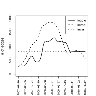
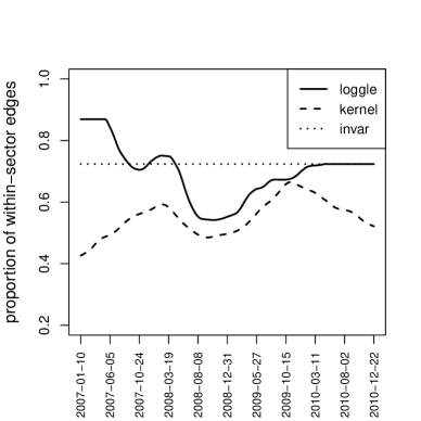
(a)	(b)

Figure 1: Stock Price. (a) Number of edges vs. time (b) Proportion of within-sector edges vs. time

Figure 1(a) shows the number of edges in the fitted graph over time. The invar fitted graphs have an identical topology, which is unable to reflect the evolving relationships among these stocks. On the other hand, both loggle and kernel are able to capture the changing relationships by fitting graphs with time-varying topologies. More specifically, both methods detect an increased amount of interaction (characterized by larger number of edges) during the financial crisis. The amount of interaction peaked around the end of 2008 and then went down to a level still higher than that of the pre-crisis period. As can be seen from the figure, the kernel graphs show rather drastic changes, whereas the loggle graphs change more gradually. The loggle method in addition detects a period with increased interaction in the early stage of the financial crisis, indicated by the smaller peak around October 2007 in Figure 1(a). This is likely due to the subprime mortgage crisis which acted as a precursor of the financial crisis (Amadeo, 2017). In the period after the financial crisis, the loggle fits are similar to those of invar with a nearly constant graph topology after March 2010, indicating that the relationships among the stocks had stabilized. In contrast, kernel fits show a small bump in edge number around the middle of 2010 and decreasing amount of interaction afterwards.

Figure 1(b) displays the proportion of within-sector edges among the total number of detected edges. During the entire time period, loggle fitted graphs consistently have higher proportion of within-sector edges than that of the kernel fitted graph. For both methods, this proportion decreased during the financial crisis due to increased amount of cross-sector interaction. For loggle, the within-sector edge proportion eventually increased and stabilized after March 2010, although at a level lower than that of the pre-crisis period. In contrast, for kernel, the within-sector proportion took a downturn again after October 2009. In summary, the loggle fitted graphs are easier to interpret in terms of describing the evolving interacting relationships among the stocks and identifying the underlying sector structure of the stocks. Hereafter, we focus our discussion on loggle fitted graphs.

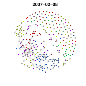
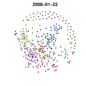
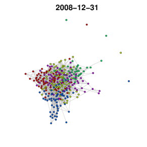
(a)	(b)	(c)
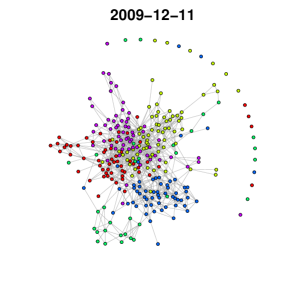
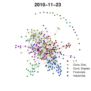
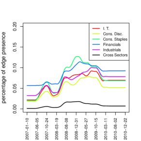
(d)	(e)	(f)

Figure 2: Stock Price. (a)-(e) loggle fitted graphs at 5 time points. (f) The sector-wise percentage of presence of within-sector edges and the percentage of presence of cross-sector edges of loggle fitted graphs vs. time.

Figure 2(a)-(e) show the loggle fitted graphs at 5 different time points, namely, before, at the early stage, around the peak, towards the end and after the financial crisis. These graphs show clear evolving interacting patterns among the stocks. The amount of interaction increased with the deepened crisis and decreased and eventually stabilized with the passing of the crisis. Moreover, the stocks have more interactions after the crisis compared to the pre-crisis era, indicating fundamental change of the financial landscape. In addition, these graphs show clear sector-wise clusters (nodes with the same color corresponding to stocks from the same sector).

Figure 2(f) shows the sector-wise percentage of presence of within-sector edges, defined as the ratio between the number of detected within-sector edges and the total number of possible within-sector edges for a given sector; and the percentage of presence of cross-sector edges, defined as the ratio between the number of detected cross-sector edges and the total number of possible cross-sector edges. As can be seen from this figure, the within-sector percentages are much higher than the cross-sector percentage, reaffirming the observation that loggle is able to identify the underlying sector structure. Moreover, the within-Financials sector percentage is among the highest across the entire time period, indicating that the stocks in this sector have been consistently highly interacting with each other. Finally, all percentages increased after the financial crisis began and leveled off afterwards, reflecting the increased amount of interaction during the financial crisis.

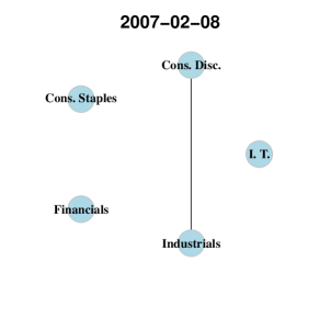
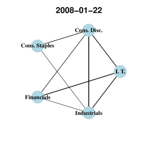
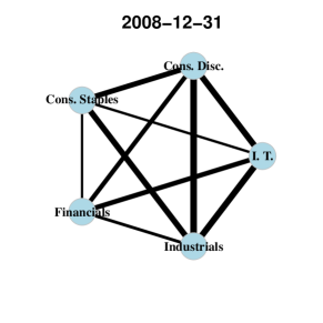
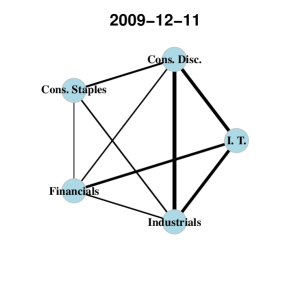
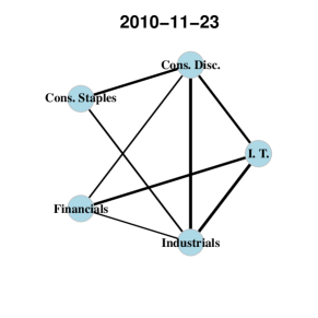
Figure 3: Stock Price. Cross-sector interaction plots at 5 different time points based on loggle fitted graphs. Each node represents a sector and the edge width is proportional to the percentage of presence of the corresponding cross-sector edges.

In Figure 3, the graphs describe cross-sector interactions among the 5 GICS sectors at five different time points (before, at early stage, around the peak, at late stage and after the financial crisis). In these graphs, each node represents a sector and edge width is proportional to the respective percentage of presence of cross-sector edges (defined as the detected number of edges between two sectors divided by the total number of possible edges between these two sectors). Moreover, edges with cross-sector percentage less than $0.2\%$ are not displayed. We can see that there are more cross-sector interactions during the financial crisis, indicating higher degree of dependency among different sectors in that period. There are also some interesting observations with regard to how these sectors interact with one another and how such interactions change over time. For example, strong cross-sector interactions between the Financials sector and the Consumer Staples sector arose during the financial crisis despite of their weak relationship before and after the crisis. This is probably due to strong influence of the financial industry on the entire economy during financial crisis. Take the Consumer Discretionary sector and the Industrials sector as another example. These two sectors maintained a persistent relationship throughout the four years, indicating intrinsic connections between them irrespective of the financial landscape.

5 Conclusion

In this paper, we propose LOcal Group Graphical Lasso Estimation – loggle, a novel model for estimating a sequence of time-varying graphs based on temporal observations. By using a local group-lasso type penalty, loggle imposes structural smoothness on the estimated graphs and consequently leads to more efficient use of the data as well as more interpretable graphs. Moreover, loggle can adapt to the local degrees of smoothness and sparsity of the underlying graphs in a data driven fashion and thus is effective under a wide range of scenarios. We develop a computationally efficient algorithm for loggle that utilizes the block-diagonal structure and pseudo-likelihood approximation. The effectiveness of loggle is demonstrated through simulation experiments. Moreover, by applying loggle to the S&P 500 stock price data, we obtain interpretable and insightful graphs about the dynamic interacting relationships among the stocks, particularly on how such relationships change in response to the recent global financial crisis. An R package loggle has been developed and will be available on http://cran.r-project.org/.

Appendix

A.1 Proof of Theorem 2

By the KKT conditions, a necessary and sufficient set of conditions for $\hat{\mathbb{\Omega}}_{k}=\{\hat{\bm{\Omega}}(t_{i})\}_{i\in\mathcal{N}_{k,d}}$ being the minimizer of $L(\mathbb{\Omega}_{k})$ in (1) is:

$$\frac{1}{\sqrt{|\mathcal{N}_{k,d}|}}\left(\hat{\bm{\Sigma}}(t_{i})-\hat{\bm{\Omega}}(t_{i})^{-1}\right)+\lambda\bm{\Gamma}(t_{i})=\bm{0},\ \forall i\in\mathcal{N}_{k,d},$$ (A.1)

where $\bm{\Gamma}(t_{i})=(\Gamma_{uv}(t_{i}))_{p\times p}$, and $(\Gamma_{uv}(t_{i}))_{i\in\mathcal{N}_{k,d}}$ is a subgradient of $\sqrt{\sum_{i\in\mathcal{N}_{k,d}}\Omega_{uv}(t_{i})^{2}}$:

$$(\Gamma_{uv}(t_{i}))_{i\in\mathcal{N}_{k,d}}\begin{cases}=\left(\frac{\Omega_{uv}(t_{i})}{\sqrt{\sum_{i\in\mathcal{N}_{k,d}}\Omega_{uv}(t_{i})^{2}}}\right)_{i\in\mathcal{N}_{k,d}}&\text{if}\ \sum_{i\in\mathcal{N}_{k,d}}\Omega_{uv}(t_{i})^{2}>0\\ \text{such that}\ \sum_{i\in\mathcal{N}_{k,d}}\Gamma_{uv}(t_{i})^{2}\leq 1&\text{if}\ \sum_{i\in\mathcal{N}_{k,d}}\Omega_{uv}(t_{i})^{2}=0.\end{cases}$$

If for $\forall i\in\mathcal{N}_{k,d}$, $\hat{\bm{\Omega}}(t_{i})=\left(\begin{array}[]{c c}\hat{\bm{\Omega}}_{1}(t_{i})&\bm{0}\\ \bm{0}&\hat{\bm{\Omega}}_{2}(t_{i})\end{array}\right)$, where $\hat{\bm{\Omega}}_{1}(t_{i})$ and $\hat{\bm{\Omega}}_{2}(t_{i})$ consist of the variables in $G_{1}$ and $G_{2}$ respectively, then $\hat{\mathbb{\Omega}}_{k}=\{\hat{\bm{\Omega}}(t_{i})\}_{i\in\mathcal{N}_{k,d}}$ satisfies (A.1) iff $\forall u\in G_{1}$, $\forall v\in G_{2}$, $\exists$ $(\Gamma_{uv}(t_{i}))_{i\in\mathcal{N}_{k,d}}$ satisfying $\sum_{i\in\mathcal{N}_{k,d}}\Gamma_{uv}(t_{i})^{2}\leq 1$ such that

$$\frac{1}{\sqrt{|\mathcal{N}_{k,d}|}}\hat{\Sigma}_{uv}(t_{i})+\lambda\Gamma_{uv}(t_{i})=0,\ \forall i\in\mathcal{N}_{k,d}.$$

This is equivalent to

$$\forall u\in G_{1},\ \forall v\in G_{2},\ \frac{1}{|\mathcal{N}_{k,d}|}\sum_{i\in\mathcal{N}_{k,d}}\hat{\Sigma}_{uv}(t_{i})^{2}\leq\lambda^{2}.$$

A.2 ADMM algorithm under pseudo-likelihood approximation

To solve the optimization problem in (4) using ADMM algorithm, we notice that the problem can be written as

$$\textrm{minimize }_{\mathbb{B}_{k},\mathbb{Z}_{k}}\sum_{i\in\mathcal{N}_{k,d}}\frac{1}{2}||\mathbf{Y}(t_{i})-\mathbf{X}(t_{i})\bm{\beta}(t_{i})||_{2}^{2}+\lambda\sum_{u<v}\sqrt{\sum_{i\in\mathcal{N}_{k,d}}\left[Z_{uv}(t_{i})^{2}+Z_{vu}(t_{i})^{2}\right]},$$

$$\textrm{subject to }\bm{\beta}(t_{i})-\bm{Z}(t_{i})=\bm{0},\;i\in\mathcal{N}_{k,d},$$

where $\mathcal{N}_{k,d}=\{i:|t_{i}-t_{k}|\leq d\}$, $\mathbb{B}_{k}=\{\bm{\beta}(t_{i})\}_{i\in\mathcal{N}_{k,d}}$ and $\mathbb{Z}_{k}=\{\bm{Z}(t_{i})\}_{i\in\mathcal{N}_{k,d}}$. Note $\bm{\beta}(t_{i})=(\beta_{uv}(t_{i}))_{u\neq v}$ and $\bm{Z}(t_{i})=(Z_{uv}(t_{i}))_{u\neq v}$ are $\mathbb{R}^{p(p-1)}$ vectors.

The scaled augmented Lagrangian is

$$L_{\rho}(\mathbb{B}_{k},\mathbb{Z}_{k},\mathbb{U}_{k})= \sum_{i\in\mathcal{N}_{k,d}}\frac{1}{2}||\mathbf{Y}(t_{i})-\mathbf{X}(t_{i})\bm{\beta}(t_{i})||_{2}^{2}+\lambda\sum_{u<v}\sqrt{\sum_{i\in\mathcal{N}_{k,d}}\left[Z_{uv}(t_{i})^{2}+Z_{vu}(t_{i})^{2}\right]}$$

$$+\frac{\rho}{2}\sum_{i\in\mathcal{N}_{k,d}}||\bm{\beta}(t_{i})-\bm{Z}(t_{i})+\bm{U}(t_{i})||_{2}^{2},$$

where $\mathbb{U}_{k}=\{\bm{U}(t_{i})\}_{i\in\mathcal{N}_{k,d}}$ are dual variables ($\bm{U}(t_{i})=(U_{uv}(t_{i}))_{u\neq v}\in\mathbb{R}^{p(p-1)}$).

The ADMM algorithm is as follows. We first initialize $\bm{Z}^{(0)}(t_{i})=\bm{0}$, $\bm{U}^{(0)}(t_{i})=\bm{0}$, $i\in\mathcal{N}_{k,d}$. We also need to specify $\rho(>0)$, which in practice is recommended to be $\approx\lambda$ (Wahlberg et al., 2012). For step $s=1,2,\ldots$ until convergence:

1. For $i\in\mathcal{N}_{k,d}$,

   $$\bm{\beta}^{s}(t_{i})=\arg\min_{\bm{\beta}(t_{i})}\frac{1}{2}||\mathbf{Y}(t_{i})-\mathbf{X}(t_{i})\bm{\beta}(t_{i})||_{2}^{2}+\frac{\rho}{2}||\bm{\beta}(t_{i})-\bm{Z}^{s-1}(t_{i})+\bm{U}^{s-1}(t_{i})||_{2}^{2}.$$

   The solution $\bm{\beta}^{s}(t_{i})$ sets the derivative of the objective function to 0:

   $$(\mathbf{X}(t_{i})^{T}\mathbf{X}(t_{i})+\rho\bm{I})\bm{\beta}^{s}(t_{i})=\mathbf{X}(t_{i})^{T}\mathbf{Y}(t_{i})+\rho(\bm{Z}^{s-1}(t_{i})-\bm{U}^{s-1}(t_{i})).$$

   It is easy to see that

   $$\mathbf{X}(t_{i})^{T}\mathbf{X}(t_{i})+\rho\bm{I}={\rm diag}\{\tilde{\mathbf{X}}_{(-u)}(t_{i})^{T}\tilde{\mathbf{X}}_{(-u)}(t_{i})+\rho\bm{I}\}_{1\leq u\leq p}={\rm diag}\{(\hat{\bm{\Sigma}}(t_{i})+\rho\bm{I})_{(-u,-u)}\}_{1\leq u\leq p},$$

   where $\hat{\bm{\Sigma}}(t_{i})$ is the kernel estimate of the covariance matrix as in Section 2.1. That is, $\mathbf{X}(t_{i})^{T}\mathbf{X}(t_{i})+\rho\bm{I}$ is a block diagonal matrix with $p$ blocks, where the $u$th block, the $(p-1)\times(p-1)$ matrix $(\hat{\bm{\Sigma}}(t_{i})+\rho\bm{I})_{(-u,-u)}$, is the matrix $\hat{\bm{\Sigma}}(t_{i})+\rho\bm{I}$ with the $u$th row and the $u$th column deleted.

   Moreover,

   $$\mathbf{X}(t_{i})^{T}\mathbf{Y}(t_{i})= ((\tilde{\mathbf{X}}_{(-1)}(t_{i})^{T}\tilde{\bm{X}}_{1}(t_{i}))^{T},\ldots,(\tilde{\mathbf{X}}_{(-p)}(t_{i})^{T}\tilde{\bm{X}}_{p}(t_{i}))^{T})^{T}$$

   $$= ((\hat{\bm{\Sigma}}(t_{i})_{(-1,1)})^{T},\ldots,(\hat{\bm{\Sigma}}(t_{i})_{(-p,p)})^{T})^{T}.$$

   That is, $\mathbf{X}(t_{i})^{T}\mathbf{Y}(t_{i})$ is a $p(p-1)\times 1$ column vector consisting of $p$ sub-vectors, where the $u$th sub-vector is the $u$th column of $\hat{\bm{\Sigma}}(t_{i})$ with the $u$th element (i.e., the diagonal element) deleted.

   Since $\mathbf{X}(t_{i})^{T}\mathbf{X}(t_{i})+\rho\bm{I}$ and $\mathbf{X}(t_{i})^{T}\mathbf{Y}(t_{i})$ can be decomposed into blocks, $\bm{\beta}^{s}(t_{i})$ can be solved block-wisely:

   $$\bm{\beta}_{u}^{s}(t_{i})=((\hat{\bm{\Sigma}}(t_{i})+\rho\bm{I})_{(-u,-u)})^{-1}(\hat{\bm{\Sigma}}(t_{i})_{(-u,u)}+\rho(\bm{Z}_{u}^{s-1}(t_{i})-\bm{U}_{u}^{s-1}(t_{i}))),\ u=1,\ldots,p,$$

   where $\bm{\beta}_{u}^{s}(t_{i})=(\beta_{u1}^{s}(t_{i}),\ldots,\beta_{u,u-1}^{s}(t_{i}),\ldots,\beta_{u,u+1}^{s}(t_{i}),\ldots,\beta_{up}^{s}(t_{i}))$ is a $(p-1)\times 1$ column vector, $\bm{\beta}^{s}(t_{i})=(\bm{\beta}_{1}^{s}(t_{i})^{T},\ldots,\bm{\beta}_{p}^{s}(t_{i})^{T})^{T}$, and $\bm{Z}_{u}^{s-1}(t_{i})=(Z_{u1}^{s-1}(t_{i}),\ldots,Z_{up}^{s-1}(t_{i}))$ and $\bm{U}_{u}^{s-1}(t_{i})=(U_{u1}^{s-1}(t_{i}),\ldots,U_{up}^{s-1}(t_{i}))$ contain the corresponding elements in $\bm{Z}^{s-1}(t_{i})$ and $\bm{U}^{s-1}(t_{i})$, respectively.

   Here, we need to solve $p$ linear systems, each with $p$ equations. One way is to conduct Cholesky decompositions of the matrices $(\hat{\bm{\Sigma}}(t_{i})+\rho\bm{I})_{(-u,-u)}$, $u=1,\ldots,p$ in advance and use Gaussian elimination to solve the corresponding triangular linear systems. To do this, we apply Cholesky decomposition to $\hat{\bm{\Sigma}}(t_{i})+\rho\bm{I}$ followed by $p$ Givens rotations. This has overall time complexity $O(p^{3})$, the same as the time complexity of the subsequent $p$ applications of Gaussian eliminations. Note that, if we had performed Cholesky decomposition on each of the $(p-1)\times(p-1)$ matrix directly, the total time complexity would have been $O(p^{4})$. The details of conducting Cholesky decompositions of the matrices $(\hat{\bm{\Sigma}}(t_{i})+\rho\bm{I})_{(-u,-u)}(u=1,\ldots,p)$ through Givens rotations are given in S.1.2 of the Supplementary Material.

2. $$\mathbb{Z}_{k}^{s}=\arg\min_{\mathbb{Z}_{k}}\left[\frac{\rho}{2}\sum_{i\in\mathcal{N}_{k,d}}||\bm{Z}(t_{i})-\bm{\beta}^{s}(t_{i})-\bm{U}^{s-1}(t_{i})||_{2}^{2}+\lambda\sum_{u<v}\sqrt{\sum_{i\in\mathcal{N}_{k,d}}\left[Z_{uv}(t_{i})^{2}+Z_{vu}(t_{i})^{2}\right]}\right].$$

   For $i\in\mathcal{N}_{k,d}$, $1\leq u\neq v\leq p$, it is easy to see that

   $$Z_{uv}^{s}(t_{i})= \left(1-\frac{\lambda}{\rho\sqrt{\sum_{j\in\mathcal{N}_{k,d}}\left[(\beta_{uv}^{s}(t_{j})+U_{uv}^{s-1}(t_{j}))^{2}+(\beta_{vu}^{s}(t_{j})+U_{vu}^{s-1}(t_{j}))^{2}\right]}}\right)_{+}$$

   $$\cdot(\beta_{uv}^{s}(t_{i})+U_{uv}^{s-1}(t_{i})).$$

3. For $i\in\mathcal{N}_{k,d}$,

   $$\bm{U}^{s}(t_{i})=\bm{U}^{s-1}(t_{i})+\bm{\beta}^{s}(t_{i})-\bm{Z}^{s}(t_{i}).$$

Over-relaxation

In steps (ii) and (iii), we replace $\bm{\beta}^{s}(t_{i})$ by $\alpha\bm{\beta}^{s}(t_{i})+(1-\alpha)\bm{Z}^{s-1}(t_{i})$, where the relaxation parameter $\alpha$ is set to be 1.5. It is suggested in Boyd et al. (2011) that over-relaxation with $\alpha\in[1.5,1.8]$ can improve convergence.

Stopping criterion

The norm of the primal residual at step $s$ is $||\bm{r}^{s}||_{2}=\sqrt{\sum_{i\in\mathcal{N}_{k,d}}||\bm{\beta}^{s}(t_{i})-\bm{Z}^{s}(t_{i})||_{2}^{2}}$, and the norm of the dual residual at step $s$ is $||\bm{d}^{s}||_{2}=\sqrt{\sum_{i\in\mathcal{N}_{k,d}}||\bm{Z}^{s}(t_{i})-\bm{Z}^{s-1}(t_{i})||_{2}^{2}}$. Define the feasibility tolerance for the primal as $\epsilon^{pri}=\epsilon^{abs}\sqrt{p|\mathcal{N}_{k,d}|}+\epsilon^{rel}\max\{\sqrt{\sum_{i\in\mathcal{N}_{k,d}}||\bm{\beta}^{s}(t_{i})||_{2}^{2}},$ $\sqrt{\sum_{i\in\mathcal{N}_{k,d}}||\bm{Z}^{s}(t_{i})||_{2}^{2}}\}$, and the feasibility tolerance for the dual as $\epsilon^{dual}=\epsilon^{abs}\sqrt{p|\mathcal{N}_{k,d}|}+\epsilon^{rel}\sqrt{\sum_{i\in\mathcal{N}_{k,d}}||\bm{U}^{s}(t_{i})||_{2}^{2}}$. Here $\epsilon^{abs}$ is the absolute tolerance and in practice is often set as $10^{-5}$ or $10^{-4}$, and $\epsilon^{rel}$ is the relative tolerance and in practice is often set as $10^{-3}$ or $10^{-2}$. The stopping criterion is that the algorithm stops if and only if $||\bm{r}^{s}||_{2}\leq\epsilon^{pri}$ and $||\bm{d}^{s}||_{2}\leq\epsilon^{dual}$.

S.1 Algorithm details

S.1.1 ADMM algorithm in likelihood-based loggle

To solve the optimization problem in (1) using ADMM algorithm, we notice that the problem can be written as

$$\textrm{minimize }_{\mathbb{\Omega}_{k},\mathbb{Z}_{k}}\sum_{i\in\mathcal{N}_{k,d}}\left[\text{tr}\left(\bm{\Omega}(t_{i})\hat{\bm{\Sigma}}(t_{i})\right)-\log|\bm{\Omega}(t_{i})|\right]+\lambda\sum_{u\neq v}\sqrt{\sum_{i\in\mathcal{N}_{k,d}}Z_{uv}(t_{i})^{2}},$$

$$\textrm{subject to }\bm{\Omega}(t_{i})-\bm{Z}(t_{i})=\bm{0},\;\bm{\Omega}(t_{i})\succ\bm{0},\;i\in\mathcal{N}_{k,d},$$

where $\mathcal{N}_{k,d}=\{i:|t_{i}-t_{k}|\leq d\}$, $\mathbb{\Omega}_{k}=\{\bm{\Omega}(t_{i})\}_{i\in\mathcal{N}_{k,d}}$ and $\mathbb{Z}_{k}=\{\bm{Z}(t_{i})\}_{i\in\mathcal{N}_{k,d}}$. Note $\bm{\Omega}(t_{i})=(\Omega_{uv}(t_{i}))$ and $\bm{Z}(t_{i})=(Z_{uv}(t_{i}))$ are $\mathbb{R}^{p\times p}$ matrices.

The scaled augmented Lagrangian is

$$L_{\rho}(\mathbb{\Omega}_{k},\mathbb{Z}_{k},\mathbb{U}_{k})= \sum_{i\in\mathcal{N}_{k,d}}\left[\text{tr}\left(\bm{\Omega}(t_{i})\hat{\bm{\Sigma}}(t_{i})\right)-\log|\bm{\Omega}(t_{i})|\right]+\lambda\sum_{u\neq v}\sqrt{\sum_{i\in\mathcal{N}_{k,d}}Z_{uv}(t_{i})^{2}}$$

$$+\frac{\rho}{2}\sum_{i\in\mathcal{N}_{k,d}}||\bm{\Omega}(t_{i})-\bm{Z}(t_{i})+\bm{U}(t_{i})||_{F}^{2},$$

where $\mathbb{U}_{k}=\{\bm{U}(t_{i})\}_{i\in\mathcal{N}_{k,d}}$ are dual variables ($\bm{U}(t_{i})=(U_{uv}(t_{i}))\in\mathbb{R}^{p\times p}$).

The ADMM algorithm is as follows. We first initialize $\bm{Z}^{(0)}(t_{i})=\bm{0}$, $\bm{U}^{(0)}(t_{i})=\bm{0}$, $i\in\mathcal{N}_{k,d}$. We also need to specify $\rho(>0)$, which in practice is recommended to be $\approx\lambda$ (Wahlberg et al. 2012). For step $s=1,2,\ldots$ until convergence:

1. For $i\in\mathcal{N}_{k,d}$,

   $$\bm{\Omega}^{s}(t_{i})=\arg\min_{\bm{\Omega}(t_{i})\succ\bm{0}}\left[\text{tr}\left(\bm{\Omega}(t_{i})\hat{\bm{\Sigma}}(t_{i})\right)-\log|\bm{\Omega}(t_{i})|+\frac{\rho}{2}||\bm{\Omega}(t_{i})-\bm{Z}^{s-1}(t_{i})+\bm{U}^{s-1}(t_{i})||_{F}^{2}\right].$$

   Set the derivative to be 0, we have

   $$\hat{\bm{\Sigma}}(t_{i})-\rho(\bm{Z}^{s-1}(t_{i})-\bm{U}^{s-1}(t_{i}))=\bm{\Omega}^{-1}(t_{i})-\rho\bm{\Omega}(t_{i}).$$

   Let $\bm{Q\Lambda Q}^{T}$ denote the eigen-decomposition of $\hat{\bm{\Sigma}}(t_{i})-\rho(\bm{Z}^{s-1}(t_{i})-\bm{U}^{s-1}(t_{i}))$, where $\bm{\Lambda}={\rm diag}\{\lambda_{1},\ldots,\lambda_{p}\}$, then

   $$\bm{\Omega}^{s}(t_{i})=\bm{Q}\tilde{\bm{\Lambda}}\bm{Q}^{T},$$

   where $\tilde{\bm{\Lambda}}$ is the diagonal matrix with $j$th diagonal element $\frac{-\lambda_{j}+\sqrt{\lambda_{j}^{2}+4\rho}}{2\rho}$.

2. $$\mathbb{Z}_{k}^{s}=\arg\min_{\mathbb{Z}_{k}}\left[\frac{\rho}{2}\sum_{i\in\mathcal{N}_{k,d}}||\bm{Z}(t_{i})-\bm{\Omega}^{s}(t_{i})-\bm{U}^{s-1}(t_{i})||_{F}^{2}+\lambda\sum_{u\neq v}\sqrt{\sum_{i\in\mathcal{N}_{k,d}}Z_{uv}(t_{i})^{2}}\right].$$

   For $i\in\mathcal{N}_{k,d}$, it is easy to see that the diagonal elements

   $$Z_{uu}^{s}(t_{i})=\Omega_{uu}^{s}(t_{i})+U_{uu}^{s-1}(t_{i}),\ u=1,\ldots,p.$$

   For the off-diagonal elements, one can show that they should take the form

   $$Z_{uv}^{s}(t_{i})=\left(1-\frac{\lambda}{\rho\sqrt{\sum_{j\in\mathcal{N}_{k,d}}(\Omega_{uv}^{s}(t_{j})+U_{uv}^{s-1}(t_{j}))^{2}}}\right)_{+}(\Omega_{uv}^{s}(t_{i})+U_{uv}^{s-1}(t_{i})).$$

3. For $i\in\mathcal{N}_{k,d}$,

   $$\bm{U}^{s}(t_{i})=\bm{U}^{s-1}(t_{i})+\bm{\Omega}^{s}(t_{i})-\bm{Z}^{s}(t_{i}).$$

Note that in Step (i), the positive-definiteness constraint on $\{\bm{\Omega}(t_{i})\}_{i\in\mathcal{N}_{k,d}}$ is automatically satisfied by implementing eigen-decomposition.

Over-relaxation

In step (ii) and (iii), we replace $\bm{\Omega}^{s}(t_{i})$ by $\alpha\bm{\Omega}^{s}(t_{i})+(1-\alpha)\bm{Z}^{s-1}(t_{i})$, where the relaxation parameter $\alpha$ is set to be 1.5.

Stopping criterion

The norm of the primal residual at step $s$ is $||\bm{r}^{s}||_{F}=\sqrt{\sum_{i\in\mathcal{N}_{k,d}}||\bm{\Omega}^{s}(t_{i})-\bm{Z}^{s}(t_{i})||_{F}^{2}}$, and the norm of the dual residual at step $s$ is $||\bm{d}^{s}||_{F}=\sqrt{\sum_{i\in\mathcal{N}_{k,d}}||\bm{Z}^{s}(t_{i})-\bm{Z}^{s-1}(t_{i})||_{F}^{2}}$. Define the feasibility tolerance for the primal as $\epsilon^{pri}=\epsilon^{abs}\sqrt{p|\mathcal{N}_{k,d}|}+\epsilon^{rel}\max\{\sqrt{\sum_{i\in\mathcal{N}_{k,d}}||\bm{\Omega}^{s}(t_{i})||_{F}^{2}},$ $\sqrt{\sum_{i\in\mathcal{N}_{k,d}}||\bm{Z}^{s}(t_{i})||_{F}^{2}}\}$, and the feasibility tolerance for the dual as $\epsilon^{dual}=\epsilon^{abs}\sqrt{p|\mathcal{N}_{k,d}|}+\epsilon^{rel}\sqrt{\sum_{i\in\mathcal{N}_{k,d}}||\bm{U}^{s}(t_{i})||_{F}^{2}}$. Here $\epsilon^{abs}$ is the absolute tolerance and in practice is often set as $10^{-5}$ or $10^{-4}$, and $\epsilon^{rel}$ is the relative tolerance and in practice is often set as $10^{-3}$ or $10^{-2}$. The stopping criterion is that the algorithm stops if and only if $||\bm{r}^{s}||_{F}\leq\epsilon^{pri}$ and $||\bm{d}^{s}||_{F}\leq\epsilon^{dual}$.

S.1.2 ADMM algorithm in pseudo-likelihood-based loggle: additional details

Givens rotation

Let $\bm{A}=\hat{\bm{\Sigma}}(t_{i})+\rho\bm{I}$, a $p\times p$ positive definite matrix. We aim to efficiently obtain the Cholesky decomposition of $\bm{A}_{j}$: $\bm{A}_{j}=\bm{U}_{j}^{T}\bm{U}_{j}$, where $\bm{A}_{j}$ is a $(p-1)\times(p-1)$ matrix obtained by deleting the $j$th row and the $j$th column of $\bm{A}$, and $\bm{U}_{j}$ is an upper triangular matrix.

We first apply the Cholesky decomposition to $\bm{A}$: $\bm{A}=\bm{U}^{T}\bm{U}$, where $\bm{U}$ is an upper triangular matrix. It is easy to see that $\bm{A}_{j}=\tilde{\bm{U}}_{j}^{T}\tilde{\bm{U}}_{j}$, where $\tilde{\bm{U}}_{j}$ is a $p\times(p-1)$ matrix from deleting the $j$th column of $\bm{U}$. We then apply the Givens rotation to $\tilde{\bm{U}}_{j}$ to get its QR decomposition: $\tilde{\bm{U}}_{j}=\bm{Q}_{j}\bm{R}_{j}$, where $\bm{Q}_{j}$ is a $p\times p$ orthogonal matrix and $\bm{R}_{j}^{T}=[\bm{U}_{j}^{T},\bm{0}]$ where $\bm{U}_{j}$ is a $(p-1)\times(p-1)$ upper triangular matrix. Thus $\bm{A}_{j}=(\bm{Q}_{j}\bm{R}_{j})^{T}\bm{Q}_{j}\bm{R}_{j}=\bm{R}_{j}^{T}\bm{R}_{j}=\bm{U}_{j}^{T}\bm{U}_{j}$ is exactly the Cholesky decomposition of $\bm{A}_{j}$.

Note that the cost of Cholesky decomposition is $O(p^{3})$ and the cost of QR decomposition by Givens rotation is $O(p^{2})$, hence by using the Givens rotation, the total computational complexity for implementing $p$ Cholesky decompositions is $O(p^{3})$.

S.1.3 De-trend

Our observations $\{\bm{x}_{k}\}_{k=1,\ldots,N}$ are drawn from $\mathcal{N}_{p}(\bm{\mu}(t_{k}),\bm{\Sigma}(t_{k}))$ ($k=1,\ldots,N$) independently. For simplicity, we can assume that these observations are centered so that each $\bm{x}_{k}$ is drawn independently from $\mathcal{N}_{p}(\bm{0},\bm{\Sigma}(t_{k}))$ ($k=1,\ldots,N$). To achieve this, we first obtain a kernel estimate of the mean function $\hat{\bm{\mu}}(t)=\sum_{j=1}^{N}\omega_{h}^{t_{j}}(t)\bm{x}_{j}$ by using R package sm, where $\omega_{h}^{t_{j}}(t)=\frac{K_{h}(t_{j}-t)}{\sum_{j=1}^{N}K_{h}(t_{j}-t)}$ and $K_{h}(\cdot)$ is a normal kernel function with $h$ being its standard deviation. We then subtract the kernel estimated mean $\hat{\bm{\mu}}(t_{k})$ from $\bm{x}_{k}$ for each $k=1,\ldots,N$.

S.2 Model tuning: additional details

S.2.1 Early stopping in grid search

When the number of nodes $p$ is large, it is often very time consuming to estimate a dense graph. Moreover, when sample size is relatively small, dense models seldom lead to good cross-validation scores (so they will not be selected anyway). Thus, we will fit models for a decreasing sequence of $\lambda$ and when the edge number of the fitted graph at a $\lambda$ exceeds a prespecified threshold (e.g, 5 times of $p$), we will stop the grid search as smaller values of $\lambda$ usually lead to even denser fitted graphs.

S.2.2 Coarse grid search

To further reduce the computational cost, we implement a coarse grid search followed by a fine grid search for model tuning. Specifically, we first apply cross-validation on coarse grids to search for appropriate values of $h$, and then we use finer grids to search for good values of $d$ and $\lambda$.

S.3 Simulation: additional details

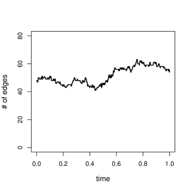
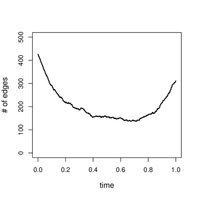
Figure S.1: Simulation. Number of edges versus time. Left: $p=100$ time-varying graphs model; Right: $p=500$ time-varying graphs model.

S.4 S&P 500 Stock Price: additional details

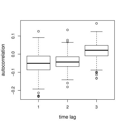
Figure S.2: Boxplots of autocorrelations at time lag 1, 2 and 3.

References

• (1)
• Ahmed & Xing (2009) Ahmed, A. & Xing, E. P. (2009), ‘Recovering time-varying networks of dependencies in social and biological studies’, Proceedings of the National Academy of Sciences 106(29), 11878–11883.
• Amadeo (2017) Amadeo, K. (2017), ‘Here’s how they missed the early clues of the financial crisis’.
https://www.thebalance.com/2007-financial-crisis-overview-3306138
• Banerjee et al. (2008) Banerjee, O., Ghaoui, L. E. & d’Aspremont, A. (2008), ‘Model selection through sparse maximum likelihood estimation for multivariate gaussian or binary data’, Journal of Machine learning research 9(Mar), 485–516.
• Boyd et al. (2011) Boyd, S., Parikh, N., Chu, E., Peleato, B. & Eckstein, J. (2011), ‘Distributed optimization and statistical learning via the alternating direction method of multipliers’, Foundations and Trends® in Machine Learning 3(1), 1–122.
• Cai et al. (2011) Cai, T., Liu, W. & Luo, X. (2011), ‘A constrained ℓ 1 minimization approach to sparse precision matrix estimation’, Journal of the American Statistical Association 106(494), 594–607.
• Danaher et al. (2014) Danaher, P., Wang, P. & Witten, D. M. (2014), ‘The joint graphical lasso for inverse covariance estimation across multiple classes’, Journal of the Royal Statistical Society: Series B (Statistical Methodology) 76(2), 373–397.
• Erdös & Rényi (1959) Erdös, P. & Rényi, A. (1959), ‘On random graphs, i’, Publicationes Mathematicae (Debrecen) 6, 290–297.
• Friedman et al. (2008) Friedman, J., Hastie, T. & Tibshirani, R. (2008), ‘Sparse inverse covariance estimation with the graphical lasso’, Biostatistics 9(3), 432–441.
• Friedman et al. (2010) Friedman, J., Hastie, T. & Tibshirani, R. (2010), Applications of the lasso and grouped lasso to the estimation of sparse graphical models, Technical report, Technical report, Stanford University.
• Gibberd & Nelson (2014) Gibberd, A. J. & Nelson, J. D. (2014), High dimensional changepoint detection with a dynamic graphical lasso, in ‘Acoustics, Speech and Signal Processing (ICASSP), 2014 IEEE International Conference on’, IEEE, pp. 2684–2688.
• Gibberd & Nelson (2017) Gibberd, A. J. & Nelson, J. D. (2017), ‘Regularized estimation of piecewise constant gaussian graphical models: The group-fused graphical lasso’, Journal of Computational and Graphical Statistics (just-accepted).
• Hallac et al. (2017) Hallac, D., Park, Y., Boyd, S. & Leskovec, J. (2017), ‘Network inference via the time-varying graphical lasso’, arXiv preprint arXiv:1703.01958 .
• Kolar et al. (2010) Kolar, M., Song, L., Ahmed, A. & Xing, E. P. (2010), ‘Estimating time-varying networks’, The Annals of Applied Statistics pp. 94–123.
• Kolar & Xing (2012) Kolar, M. & Xing, E. P. (2012), ‘Estimating networks with jumps’, Electronic journal of statistics 6, 2069.
• Lam & Fan (2009) Lam, C. & Fan, J. (2009), ‘Sparsistency and rates of convergence in large covariance matrix estimation’, Annals of statistics 37(6B), 4254.
• Meinshausen & Bühlmann (2006) Meinshausen, N. & Bühlmann, P. (2006), ‘High-dimensional graphs and variable selection with the lasso’, The annals of statistics pp. 1436–1462.
• Monti et al. (2014) Monti, R. P., Hellyer, P., Sharp, D., Leech, R., Anagnostopoulos, C. & Montana, G. (2014), ‘Estimating time-varying brain connectivity networks from functional mri time series’, NeuroImage 103, 427–443.
• Peng et al. (2009) Peng, J., Wang, P., Zhou, N. & Zhu, J. (2009), ‘Partial correlation estimation by joint sparse regression models’, Journal of the American Statistical Association 104(486), 735–746.
• Peng et al. (2010) Peng, J., Zhu, J., Bergamaschi, A., Han, W., Noh, D.-Y., Pollack, J. R. & Wang, P. (2010), ‘Regularized multivariate regression for identifying master predictors with application to integrative genomics study of breast cancer’, The annals of applied statistics 4(1), 53.
• Ravikumar et al. (2011) Ravikumar, P., Wainwright, M. J., Raskutti, G., Yu, B. et al. (2011), ‘High-dimensional covariance estimation by minimizing ℓ1-penalized log-determinant divergence’, Electronic Journal of Statistics 5, 935–980.
• Rothman et al. (2008) Rothman, A. J., Bickel, P. J., Levina, E., Zhu, J. et al. (2008), ‘Sparse permutation invariant covariance estimation’, Electronic Journal of Statistics 2, 494–515.
• Song et al. (2009) Song, L., Kolar, M. & Xing, E. P. (2009), ‘Keller: estimating time-varying interactions between genes’, Bioinformatics 25(12), i128–i136.
• Wahlberg et al. (2012) Wahlberg, B., Boyd, S., Annergren, M. & Wang, Y. (2012), ‘An admm algorithm for a class of total variation regularized estimation problems’, IFAC Proceedings Volumes 45(16), 83–88.
• Wang & Kolar (2014) Wang, J. & Kolar, M. (2014), ‘Inference for sparse conditional precision matrices’, arXiv preprint arXiv:1412.7638 .
• Wit & Abbruzzo (2015) Wit, E. C. & Abbruzzo, A. (2015), ‘Inferring slowly-changing dynamic gene-regulatory networks’, BMC bioinformatics 16(6), S5.
• Witten et al. (2011) Witten, D. M., Friedman, J. H. & Simon, N. (2011), ‘New insights and faster computations for the graphical lasso’, Journal of Computational and Graphical Statistics 20(4), 892–900.
• Yuan & Lin (2006) Yuan, M. & Lin, Y. (2006), ‘Model selection and estimation in regression with grouped variables’, Journal of the Royal Statistical Society: Series B (Statistical Methodology) 68(1), 49–67.
• Yuan & Lin (2007) Yuan, M. & Lin, Y. (2007), ‘Model selection and estimation in the gaussian graphical model’, Biometrika 94(1), 19–35.
• Zhou et al. (2010) Zhou, S., Lafferty, J. & Wasserman, L. (2010), ‘Time varying undirected graphs’, Machine Learning 80(2-3), 295–319.