Exceptional Points of Resonant States on a Periodic Slab

Abstract

A special kind of degeneracies known as the exceptional points (EPs), for resonant states on a dielectric periodic slab, are investigated. Due to their unique properties, EPs have found important applications in lasing, sensing, unidirectional operations, etc. In general, EPs may appear in non-Hermitian eigenvalue problems, including those related to $\mathcal{PT}$-symmetric systems and those for open dielectric structures (due to the existence of radiation loss). In this paper, we study EPs on a simple periodic structure: a slab with a periodic array of gaps. Using an efficient numerical method, we calculate the EPs and study their dependence on geometric parameters. Analytic results are obtained for the limit as the periodic slab approaches a uniform one. Our work provides a simple platform for further studies concerning EPs on dielectric periodic structures, their unusual properties and applications.

PACS numbers

42.65.Hw,42.25.Fx,42.79.Dj

I Introduction

In parameter-dependent eigenvalue problems of non-Hermitian operators, a special kind of degeneracy may occur at some particular values of the system parameters, that is, two or more eigenvalues coalesce and their corresponding eigenfunctions collapse into one single function. Such a spectral degeneracy is called an exceptional point (EP) Kato (1966). The EPs are interesting, because they give rise to unusual physical phenomena in many systems related to non-Hermitian eigenvalue problems Moiseyev (2011); Heiss (2012); Jones (1988); Heiss and Sannino (1990, 1991); Leyvraz and Heiss (2005); Cartarius et al. (2008). The EPs are also central to quantum or classical parity-time ($\mathcal{PT}$) symmetric systems Bender and Boettcher (1998); Bender et al. (1999). In these systems, an EP corresponds to a transition (also known as the $\mathcal{PT}$ symmetry breaking) from a state with all real eigenvalues to a state with complex eigenvalues Bender et al. (2002). In recent years, $\mathcal{PT}$-symmetric optical systems have been intensively investigated. EPs have been observed in $\mathcal{PT}$-symmetric waveguides Klaiman et al. (2008); Rüter et al. (2010), and exploited in a variety of optical systems leading to a number of unusual wave phenomena and novel applications such as the revival of lasing Liertzer et al. (2012); Peng et al. (2014); Brandstetter et al. (2014), enhanced sensing Hodaei et al. (2017); Chen et al. (2017a), stopping light pulses Goldzak et al. (2018), single mode lasers Feng et al. (2014), and unidirectional invisibility Lin et al. (2011).

Due to the outgoing radiation conditions, the eigenvalue problem of resonant modes on open structures is non-Hermitian, even if the dielectric function $\varepsilon$ of the structure is real and positive. Therefore, EPs of resonant modes could exist on properly designed passive structures. For example, a micro-toroid cavity with two nearby nanoscale scatterers was designed to have an EP, and it was used to enhance sensing Chen et al. (2017b). Periodic structures surrounded by or sandwiched between free space are also open structures. Thus, the eigenvalue problem for resonant modes on such a periodic structure is non-Hermitian and there could be EPs. In fact, EPs have been observed on a photonic crystal slab Zhen et al. (2015); Kamiński et al. (2017), and they exist for any specified wavevector direction, as far as the geometric parameters are properly chosen.

To reveal novel properties of EPs on open dielectric structures and realize their potential applications, it is necessary to carry out systematic studies on EPs. In this paper, we develop an efficient numerical method for computing second-order (i.e., doubly degenerate) EPs based on the square-root splitting of the eigenvalues, calculate the EPs on a simple dielectric periodic slab, and find out how they vary with the geometric parameters. Although the structure is very simple, many EPs exist, and they exhibit rather complicated dependence on the parameters. However, we are able to find a simple analytic result for the limit as the periodic slab approaches a uniform one. The EPs in this limit are related to artificial degeneracies of the guided modes of the uniform slab when it is regarded as a periodic one. The rest of this paper is organized as follows. In Sec. II, we give some definitions and show the band structure of a particular periodic slab. In Sec. III, we develop an efficient numerical method for computing EPs, and show the band structure of a periodic slab with one EP. In Sec. IV, we analyze the artificial degeneracies of a uniform slab. In Sec. V, we calculate the EPs on the periodic slab and show their dependence on parameters, including the limit studied in Sec. IV. Finally, we conclude our paper with some remarks in Sec. VI.

II Resonant modes

A typical periodic dielectric slab is shown in Fig. 1.

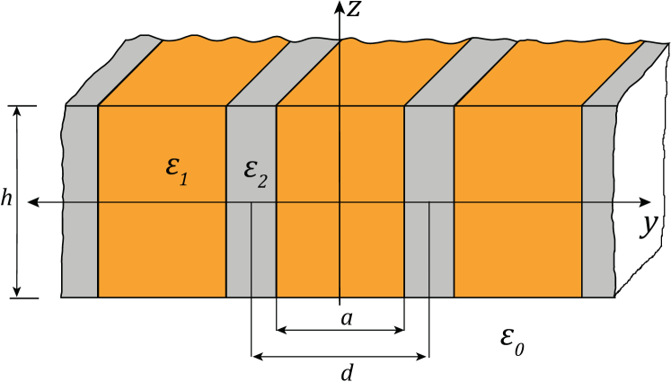
Figure 1: A dielectric slab which is invariant in $x$ and periodic in $y$. Each period consists of two segments.

The structure is invariant in $x$, periodic in $y$ with period $d$, finite in $z$ with a thickness $h$, and surrounded by air. It is further assumed that each period of the slab consists of two segments with dielectric constants $\varepsilon_{1}$ and $\varepsilon_{2}$, and widths $a$ and $d-a$, respectively. For the $E$-polarization, the $x$ component of the electric field, denoted as $u$, satisfies the following two dimensional (2D) Helmholtz equation:

$$\partial_{y}^{2}u+\partial_{z}^{2}u+k^{2}\varepsilon(y,z)u=0,$$ (1)

where $\varepsilon=\varepsilon(y,z)$ is the dielectric function of the structure, $k=\omega/c$ is the free-space wavenumber, $\omega$ is the angular frequency, and $c$ is the speed of light in vacuum.

A Bloch mode on the periodic slab is a solution of Eq. (1) given in the form

$$u(y,z)=\phi(y,z)\,e^{i\beta y},$$ (2)

where $\beta$ is a real Bloch wavenumber satisfying $\left|\beta\right|\leq\pi/d$, and $\phi(y,z)$ is periodic in $y$ with period $d$. In the free space surrounding the slab, i.e., for $\left|z\right|>h/2$, the solution can be expanded in plane waves as

$$u(y,z)=\sum_{m=-\infty}^{\infty}\hat{u}_{m}^{\pm}e^{i(\beta_{m}y\pm\alpha_{m}z)},\quad\pm z>h/2,$$ (3)

where $\hat{u}_{m}^{\pm}$ are the expansion coefficients,

$$\beta_{m}=\beta+2\pi m/d,\quad\alpha_{m}=\sqrt{k^{2}-\beta_{m}^{2}},$$ (4)

and the square root is defined with a branch cut along the negative imaginary axis.

If $\phi(y,z)\to 0$ as $\left|z\right|\to\infty$, then the Bloch mode is a guided mode. Below the light line, i.e., for $k<\left|\beta\right|$, guided modes exist continuously with respect to the frequency and the wavenumber. Above the light line, Bloch modes with the expansion (3) are typically resonant modes with a complex frequency, that is, $k$ is complex and $\mathrm{Re}(k)>\left|\beta\right|$. The resonant modes satisfy outgoing radiation conditions as $\left|z\right|\to\infty$. From Eq. (4), it is clear that $\alpha_{0}$ is a complex number with a negative imaginary part. Therefore, the plane waves $\mathrm{exp}[i(\beta y\pm\alpha_{0}z)]$ blow up as $z\to\pm\infty$, respectively. The quality factor, denoted by $Q$, of a resonant mode is given by $Q=-0.5\,\mathrm{Re}(k)/\mathrm{Im}(k)$. In special circumstances, resonant modes with infinite quality factors, i.e. $\mathrm{Im}(k)=0$, may exist, and they are the bound states in the continuum (BICs). The BICs have intriguing properties and important applications Hsu et al. (2016).

Numerical methods for computing the Bloch modes can be classified as linear and nonlinear schemes. A linear scheme discretizes the Helmholtz equation directly to obtain a linear matrix eigenvalue problem for eigenvalue $k^{2}$. A nonlinear scheme produces a nonlinear eigenvalue problem with a smaller matrix whose entries depend on $k$ implicitly. The mode matching method is a nonlinear scheme. For the structure shown in Fig. 1, it gives rise to a homogeneous linear system ${\bm{A}}(\beta,k){\bm{x}}={\bm{0}}$, where ${\bm{x}}$ is a vector of unknown expansion coefficients. For a given $\beta$, nontrivial solutions can be found by searching complex $k$ such that $\lambda_{1}({\bm{A}})=0$, where $\lambda_{1}({\bm{A}})$ is the eigenvalue of ${\bm{A}}$ with the smallest magnitude. Additional details about the numerical methods are given in Appendix A.

As a numerical example, we show the band structure of a periodic slab with $\varepsilon_{1}=15.42$, $\varepsilon_{2}=1$, $a=0.5d$ and $h=1.16d$ in Fig. 2.

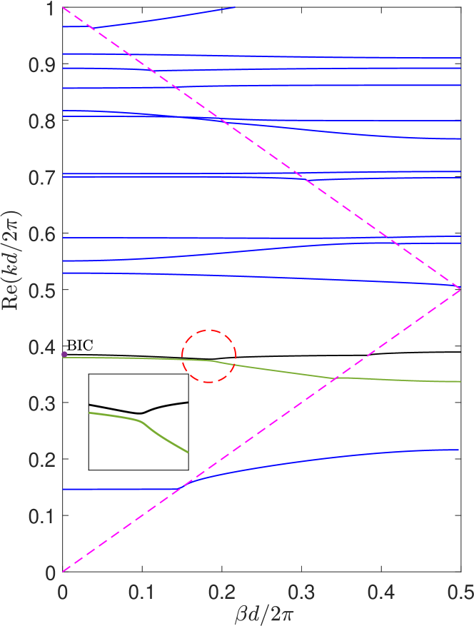
Figure 2: Band structure of Bloch modes (odd in $z$) on a periodic slab with $\varepsilon_{1}=15.42$, $\varepsilon_{2}=1$, $a=0.5d$ and $h=1.16d$.

To obtain these results, we first use a linear scheme to calculate the eigenmodes at $\beta=0$, and then use the more accurate mode matching method to find each band for $0<\beta\leq\pi/d$. For simplicity, we only show $\mathrm{Re}(k)$ for resonant modes that are odd functions of $z$. Notice that two curves, the solid black one and the solid green one, are close to each other at $\beta\approx 0.18(2\pi/d)$. In Fig. 3,

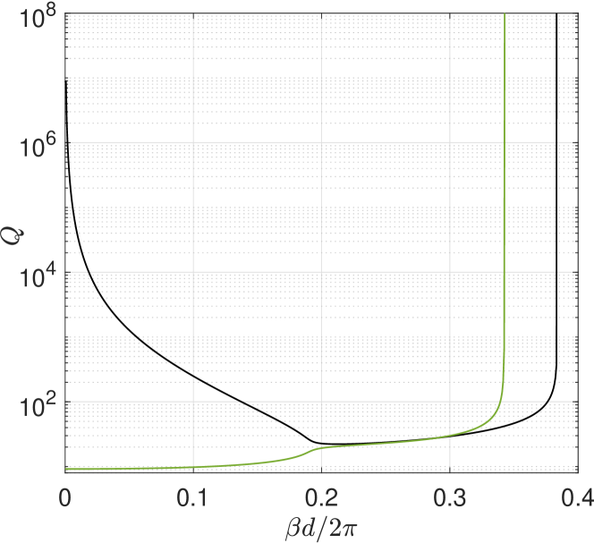
Figure 3: Quality factors of the resonant modes corresponding to the black and green curves in Fig. 2.

we show the quality factors of the resonant modes corresponding to these two curves. It can be seen that the quality factors are also close to each other at $\beta\approx 0.18(2\pi/d)$. Notice that the quality factor of the black curve diverges at $\beta=0$, and this corresponds to a BIC at $\beta=0$, i.e., a standing wave. Meanwhile, the quality factors of both curves diverge as the pair $(\beta,k)$ approaches the light line.

In the next section, we show that by tuning one structural parameter, these two resonant modes can be forced to coalesce, giving rise to a second-order EP.

III Exceptional Points

If two eigenvalues, say $k_{+}$ and $k_{-}$, are close to each other for some $\beta$, there may be an EP on a structure with slightly different parameters. To find the EP, we can try to find the parameter values and $\beta$, such that $k_{+}=k_{-}$, and check whether the eigenfunctions also coalesce. This approach is tedious and inefficient. In the following, we develop an efficient method based on the square-root splitting of the eigenvalues at second-order EPs.

Let $k_{*}$ and $\beta_{*}$ be the eigenvalue and Bloch wavenumber of a second-order EP associated with the bands $k_{+}(\beta)$ and $k_{-}(\beta)$. In the vicinity of the EP, the eigenvalues have the following approximations

$$k_{\pm}(\beta)\approx k_{*}\pm(b_{1}+i\,b_{2})\sqrt{\beta-\beta_{*}},\quad\beta>\beta_{*},$$ (5)

$$k_{\pm}(\beta)\approx k_{*}\pm(c_{1}+i\,c_{2})\sqrt{\beta_{*}-\beta},\quad\beta<\beta_{*},$$ (6)

where $b_{1}$, $b_{2}$, $c_{1}$ and $c_{2}$ are unknown real constants. Since the EP is a resonant mode with $\beta=\beta_{*}$ and $k=k_{*}$, we have

$$\lambda_{1}\left[{\bm{A}}(\beta_{*},k_{*})\right]=0,$$ (7)

where ${\bm{A}}(\beta,k)$ is a matrix obtained by the mode matching method (see Appendix A). In addition, for a small $\delta\beta>0$, two resonant modes exist at $\beta=\beta_{*}+\delta\beta$ with $k_{\pm}(\beta)$ given by Eq. (5). This leads to

$$\lambda_{1}\left[{\bm{A}}(\beta_{*}+\delta\beta,k_{*}+\delta k)\right]\approx 0,$$ (9)

$$\lambda_{1}\left[{\bm{A}}(\beta_{*}+\delta\beta,k_{*}-\delta k)\right]\approx 0,$$

where $\delta k=(b_{1}+ib_{2})\sqrt{\delta\beta}$. Therefore, we can find second-order EPs by choosing a proper $\delta\beta$ and solving Eqs. (7), (9) and (9). It turns out that EPs can be found by tuning just one structural parameter. If $\varepsilon_{1}$, $\varepsilon_{2}$ and $a$ are fixed, we can search the slab thickness $h$ to find EPs. The three complex equations (7), (9) and (9), corresponding to six real equations, are used to determine six real unknowns: $\left\{h_{*},\beta_{*},\mathrm{Re}(k_{*}),\mathrm{Im}(k_{*}),b_{1},b_{2}\right\}$, where $h_{*}$ denotes the particular value of $h$ for EPs. The values of $b_{1}$ and $b_{2}$ describe how strongly the modes split from the EP as $\beta$ moves away from $\beta_{*}$.

Following the example in Sec. II, we choose $\varepsilon_{1}=15.42$, $\varepsilon_{2}=1$ and $a=0.5d$, and allow $h$ to vary. Using the method described above, we found an EP for $h_{*}=1.154485\,d$, $\beta_{*}=0.187005(2\pi/d)$ and $k_{*}=(0.3761904-0.0092194i)\,(2\pi/d)$. The band structure of the period slab with thickness $h_{*}$ is shown in

Figure 4: Band structure of Bloch modes on a periodic slab with $\varepsilon_{1}=15.42$, $\varepsilon_{2}=1$, $a=0.5d$ and $h_{*}=1.154485d$.

Fig. 4. It is clear that two two bands touch at the EP with a square-root splitting in the vicinity of $\beta_{*}$. The quality factors of these two bands are shown in Fig. 5.

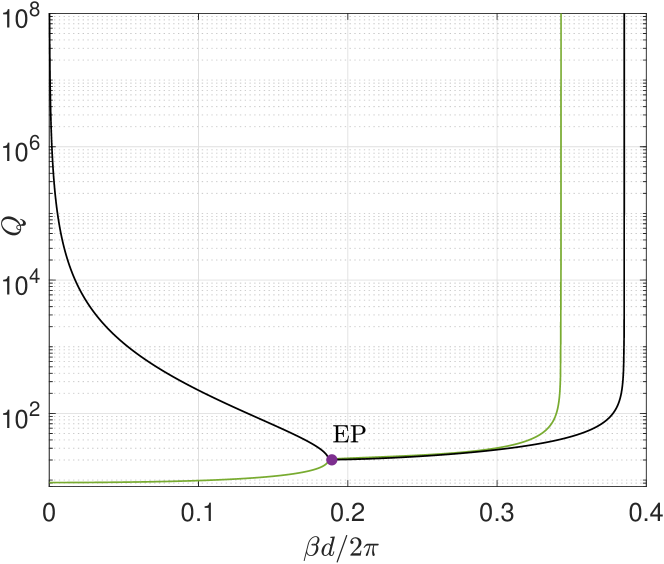
Figure 5: Quality factors of the resonant modes corresponding to black and green curves in Fig. 4.

As expected, the two curves in Fig. 5 also touch at $\beta_{*}$.

It should be pointed out that an EP can be calculated by using either Eq. (5) or Eq. (6). For the latter case, we choose a negative $\delta\beta$ and calculate the constants $c_{1}$ and $c_{2}$. It turns out that these constants satisfy

$$c_{1}=\pm b_{2},\quad\mathrm{and}\quad c_{2}=\mp b_{1}.$$ (10)

More features of the EPs can be understood by closely examining the behavior of the eigenmodes in the vicinity of $\beta_{*}$. In Fig. 6(a), we show the real and imaginary parts of $k$ for two resonant modes around the EP.

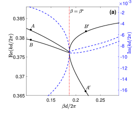
(a)

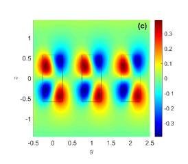
(b)

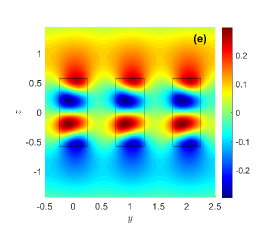
(c)

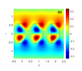
(d)

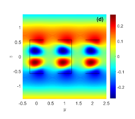
(e)

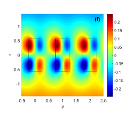
(f)

Figure 6: (a) Dispersion curves around an EP with $\beta_{*}=0.187005\,(2\pi/d)$. (b) The eigenfunction of the EP solution. (c), (d), (e), (f) The eigenfunctions at points $A$, $B$, $B^{\prime}$, $A^{\prime}$ shown in (a), respectively.

In Figs. 6(c) and 6(d), we show the two eigenfunctions, $\phi_{+}$ and $\phi_{-}$, corresponding to points $A$ and $B$ in Fig. 6(a), respectively. As $\beta\to\beta_{*}$, those two eigenfunctions coalesce into a single EP eigenfunction $\phi_{*}$ as shown in Fig. 6(b). Notice that the field pattern of $\phi_{*}$ combines the main features of $\phi_{-}$ and $\phi_{+}$. For $\beta>\beta_{*}$, two different eigenfunctions are recovered, and they are shown in Figs. 6(e) and 6(f), corresponding to points $B^{\prime}$ and $A^{\prime}$ in Fig. 6(a), respectively. Notice that the field patterns for points $A$ and $A^{\prime}$ are similar, and those for $B$ and $B^{\prime}$ are also similar, but their ordering with respect to $\mathrm{Re}(k)$ is reversed. This switching behavior of the field patterns as $\beta$ passes through $\beta_{*}$ is consistent with Eq. (10).

To develop a better understanding about EPs on the periodic slab, we will analyze their dependence on parameter $a$ in Sec. V. It will be shown that these EPs continue to exist as $a\to d$, and their $\beta_{*}$ and $k_{*}$ approach the light line. It also appears that the limiting points on the light line are related to some artificial degeneracies of the uniform slab when it is regarded as a periodic structure. In the next section, we study these artificial degeneracies and calculate the limiting points on the light line.

IV Uniform slab

Referring to Fig. 1, by setting $a=d$, we have a uniform slab with $\varepsilon=\varepsilon_{1}$. A guided mode is now given by

$$u(y,z)=\tilde{\phi}(z)e^{i\tilde{\beta}y},$$ (11)

where $\tilde{\beta}$ is the propagation constant, and $\tilde{\phi}$ satisfies

$$\frac{d^{2}\tilde{\phi}}{dz^{2}}+k^{2}\varepsilon(z)\tilde{\phi}=\tilde{\beta}^{2}\tilde{\phi},$$ (12)

where $\varepsilon(z)=\varepsilon_{1}$ for $|z|<h/2$ and $\varepsilon(z)=1$ for $|z|>h/2$. In addition, $\tilde{\phi}$ must decay to zero as $\left|z\right|\to\infty$. As in previous sections, we only consider the modes that are odd in $z$, and denote their dispersion relations as $k=k_{m}(\tilde{\beta})$ for positive integers $m$. It is straightforward to show that these dispersion curves touch the light line when

$$\tilde{\beta}=k_{m}(\tilde{\beta})=\tilde{\beta}_{m}\triangleq\frac{2\pi(m-1/2)}{h\sqrt{\varepsilon_{1}-1}}.$$ (13)

The uniform slab can be regarded as a periodic structure with a fictitious period $d$, then the guided modes can be written as $u(y,z)=\phi(y,z)\exp(i\beta y)$, where

$$\phi(y,z)=\tilde{\phi}(z)e^{i2\pi\,l\,y/d},\quad\beta=\tilde{\beta}-2\pi l/d,$$

for some integer $l$ such that $\beta\in[-\pi/d,\pi/d]$. If $|\tilde{\beta}|\leq\pi/d$, then $l=0$ and $\beta=\tilde{\beta}$. Otherwise, $l$ is nonzero and the dispersion curves of the fictitious periodic slab can be obtained by folding the dispersion curves of the uniform slab into the first Brillouin zone. This is shown in Fig. 7

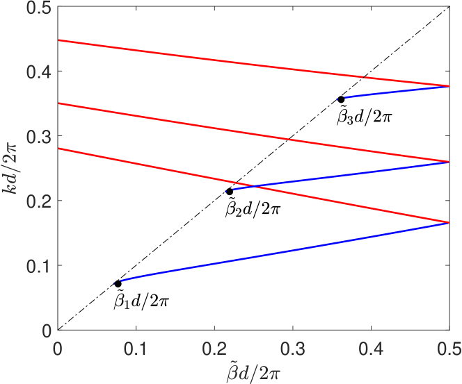
Figure 7: Folded band structure of a uniform slab with $h=1.85\,d$.

for $h=1.85\,d$, where the solid blue and red curves correspond to $l=0$ and $l=1$, respectively. More precisely, the sold red curves are

$$k=k_{m}^{({\rm f})}(\beta)\triangleq k_{m}(2\pi/d-\beta).$$

For the case shown in Fig. 7, the dispersion curves have no intersections on the light line. However, it is possible to have intersections on the light line if we tune the value of $h$. In general, we have the following “limiting degeneracy problem”:

Given integers $m>n>0$, find $h_{*}$ such that

$$k_{n}(2\pi/d-\tilde{\beta}_{m})=\tilde{\beta}_{m}.$$ (14)

For $m=2$ and $n=1$, we solve the above problem and obtain $h_{*}=1.7137192\,d$. In Fig. 8,

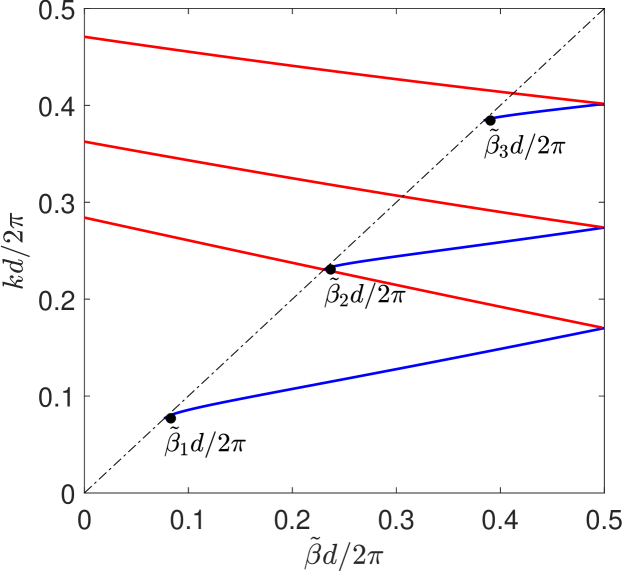
Figure 8: Folded band structure of a uniform slab with $h=1.7137192\,d$.

the dispersion curves are shown for this $h_{*}$, and the intersection on the light line is $k_{*}=\beta_{*}=0.2304989\,(2\pi/d)$. The results for different pairs $(m,n)$ are listed in Table 1.

Table 1: Solutions of the “limiting degeneracy problem”.

$(m,n)$	$h_{*}/d$	$k_{*}d/2\pi$
$(2,1)$	1.7137192	0.2304989
$(3,1)$	3.0874410	0.2132351
$(3,2)$	2.5587359	0.2572953
$(4,1)$	4.4232537	0.2083741
$(4,2)$	4.0470027	0.2277466
$(4,3)$	3.3127043	0.2782292
$(5,1)$	5.7438584	0.2063128
$(5,2)$	5.4487877	0.2174853
$(5,3)$	4.9112722	0.2412881
$(5,4)$	4.0155953	0.2951073

V Continuation of EPs

In Sec. III, we presented one EP for a periodic slab with $a=0.5d$. In fact, many different EPs can be found for the same $a$, but typically for different slab thickness. To get a more complete picture about the EPs on the periodic slab, we use the numerical method of Sec. III to follow the EPs in the parameter space of $a$ and $h$, while keeping $\varepsilon_{1}=15.42$ and $\varepsilon_{2}=1$ fixed. For simplicity, only those resonant modes that are odd in $z$ are considered. The results are shown in Figs. 9, 10 and 11

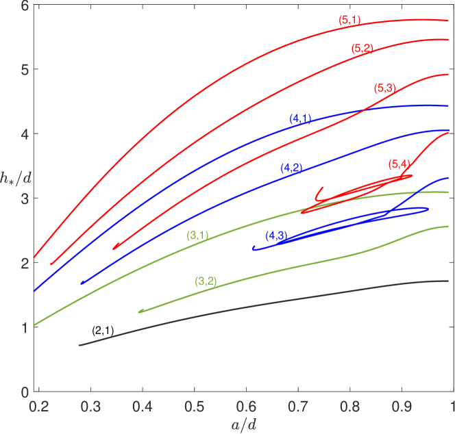
Figure 9: Slab thickness $h_{*}$ versus width $a$ for EPs satisfying $\beta_{*}<\mbox{Re}(k_{*})<2\pi/d-\beta_{*}$.

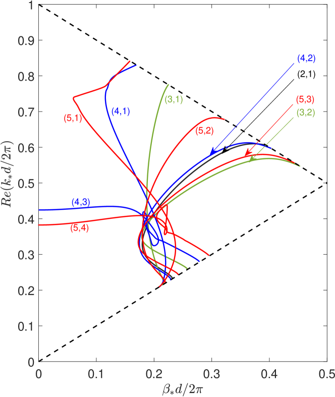
Figure 10: Eigenvalue $k_{*}$ versus wavenumber $\beta_{*}$ for the same EPs as shown in Fig. 9. The curves tend to the light line as $a\to d$.

Figure 11: Quality factors versus $a$ for the same EPs as shown in Fig. 9. The quality factors diverge as $a\to d$.

for $h_{*}$ vs. $a$, $\mbox{Re}(k_{*})$ vs. $\beta_{*}$, and quality factor vs. $a$, respectively.

In Fig. 9, we show ten curves in the $a\textendash h$ plane, where each curve represents one family of EPs that depend continuously on $a$ and $h$. These curves are labeled by pairs of integers $(m,n)$. Notice that as $a\to d$, all these curves tend to the values of $h_{*}$ listed in Table 1, according to their corresponding labels. The $\beta_{*}$ and $k_{*}$ values of the ten families of EPs are shown in Fig. 10. As $a\to d$, the curves in Fig. 10 approach the light line exactly at the values of $k_{*}$ listed in Table 1. Therefore, it can be argued that all these EPs originate from the artificial degeneracies of the guided modes on the uniform slab. In Fig. 9, we observe that different curves, e.g., $(4,1)$ and $(5,3)$, may intersect. This simply means that for the same periodic slab, there are two EPs with different $\beta_{*}$ and $k_{*}$. Notice that the curves $(4,3)$ and $(5,4)$ can intersect with themselves. On a periodic slab corresponding to such an intersection, there are two EPs that belong to the same family, but their $\beta_{*}$ and $k_{*}$ are again different. The left end points of the curves in Fig. 9 correspond to either $\beta_{*}=0$, or $\beta_{*}=2\pi/d-\mbox{Re}(k_{*})$ which is the opening line of the second radiation channel. EPs exist beyond this line, but they tend to have lower quality factors. The quality factors of the ten families of EPs are shown in Fig. 11. It can be observed that the quality factors of all EPs diverge as $a\to d$, and they are relatively small for smaller values of $a$.

In Fig. 12,

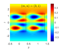
(a)

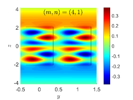
(b)

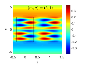
(c)

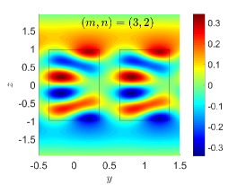
(d)

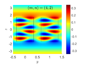
(e)

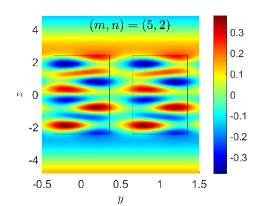
(f)

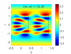
(g)

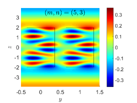
(h)

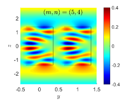
(i)

Figure 12: Eigenfunctions $\phi_{*}$ for EPs on periodic slabs with $a=0.7d$ and different $h_{*}$. The EPs are labeled by integer pairs $(m,n)$ as in Fig. 9.

we show the field patterns of nine EPs on periodic slabs with $a=0.7d$. The case for $(m,n)=(2,1)$ is not shown, since it is similar to the one in Fig. 6(b) for $a=0.5d$. Notice that different scales in $z$ are used in the different panels, since the values of $h_{*}$ are different for different EPs. It should be pointed out that the wave field pattern varies continuously on each curve shown in Fig. 9, and the main features, such as the number of polarity changes along the $y$ and $z$ axes, are preserved when $(a,h_{*})$ moves along each curve.

Near a second-order EP, the dispersion curves exhibit a square-root splitting. One example is shown in Fig. 6(a), where a square-root splitting can be observed for both real and imaginary parts of $k$, and for both $\beta>\beta_{*}$ and $\beta<\beta_{*}$. For this particular case, $\mbox{Re}(k)$ has a stronger splitting for $\beta>\beta_{*}$, and $\mbox{Im}(k)$ has a stronger splitting for $\beta<\beta_{*}$, since $|b_{1}|=|c_{2}|>|b_{2}|=|c_{1}|$. For some special EPs, $b_{1}$ or $b_{2}$ can be exactly zero. In Figs. 13 (a) and 13(b),

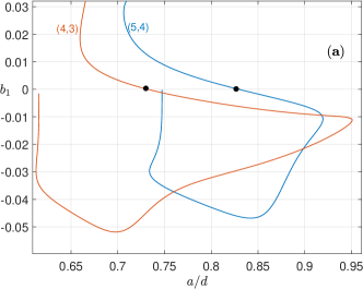
(a)

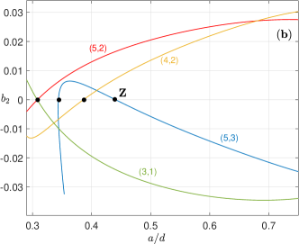
(b)

Figure 13: (a) Coefficient $b_{1}$ versus $a$. (b) Coefficient $b_{2}$ versus $a$. Solid black dots are zeros of $b_{1}$ or $b_{2}$.

we show $b_{1}$ and $b_{2}$ vs. $a$ for a few families of EPs. It is clear that $b_{1}$ or $b_{2}$ can be zero for some special values of $a$. If $b_{1}$ or $b_{2}$ is zero, the square-root splitting becomes one-sided. For example, if $b_{2}=c_{1}=0$, then $\mathrm{Re}(k)$ has a square-root splitting only for $\beta>\beta_{*}$, and $\mathrm{Im}(k)$ has a square-root splitting only for $\beta<\beta_{*}$. A particular example is shown in Fig. 14,

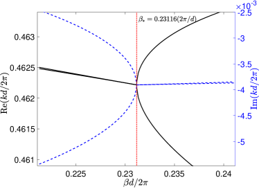
(a)

Figure 14: One-sided square-root splitting of $\mathrm{Re}(k)$ (solid black curves) and $\mathrm{Im}(k)$ (dashed blue curves) for an EP with $b_{2}=0$, i.e., point $Z$ in Fig. 13 (b).

and it corresponds to point $Z$ marked in Fig. 13(b). Actually, even though $b_{2}=0$, $\mathrm{Im}(k)$ still shows a splitting for $\beta>\beta_{*}$, but it is a weaker linear splitting proportional to $\beta-\beta_{*}$. The same is true for $\mathrm{Re}(k)$ and $\beta<\beta_{*}$.

VI Conclusion

Electromagnetic resonant modes on open dielectric structures are solutions of a non-Hermitian eigenvalue problem derived from the Maxwell’s equations. EPs of resonant modes are special degenerate states for which both the eigenvalues and the eigenfunctions coalesce. In optical systems, EPs have given rise to many interesting wave phenomena and some important applications. In this paper, we investigated exceptional points on a simple dielectric periodic slab. An efficient numerical method for computing second-order EPs was developed and used to calculate families of EPs that vary continuously with structural parameters. Due to the extra degree of freedom related to the Bloch wavenumber, it is possible to find EPs by tuning only one parameter of the periodic structure. It is worth mentioning that analytic results have been obtained for the limit $a\to d$, i.e., the periodic slab approaching a uniform one. It was shown that the EPs tend to some points on the light line in this limit, and these points are related to some artificial degeneracies of the band structure of a uniform slab when it is regarded as a periodic one.

Our results show that the EPs have rather complicated dependence on the geometric parameters of the periodic slab. For simplicity, we have concentrated on the odd resonant modes in the $E$ polarization for a very simple periodic slab. Further studies are needed to understand EPs on more general and three-dimensional structures, to reveal their properties including existence and robustness, to find out their impact on transmission spectra, reflection spectra and field enhancement, and to realize more valuable applications.

Appendix A Numerical methods

The eigenvalue problem for resonant modes on the periodic slab can be solved by a linear scheme based on the Chebyshev pseudospectral method Trefethen (2000) and the perfectly matched layer (PML) technique Berenger (1994); Chew and Weedon (1994). For the periodic function $\phi$ given in Eq. (2), the Helmholtz equation (1) becomes

$$\frac{\partial^{2}\phi}{\partial z^{2}}+\frac{\partial^{2}\phi}{\partial y^{2}}+2i\beta\frac{\partial\phi}{\partial y}-\beta^{2}\phi=-k^{2}\varepsilon\phi.$$ (15)

If the modes are odd in $z$, it is only necessary to consider $z>0$ together with a zero boundary condition at $z=0$. The $z$ axis is truncated at $z=z_{2}$ with a PML for $z_{1}<z<z_{2}$ as shown in Fig. 15.

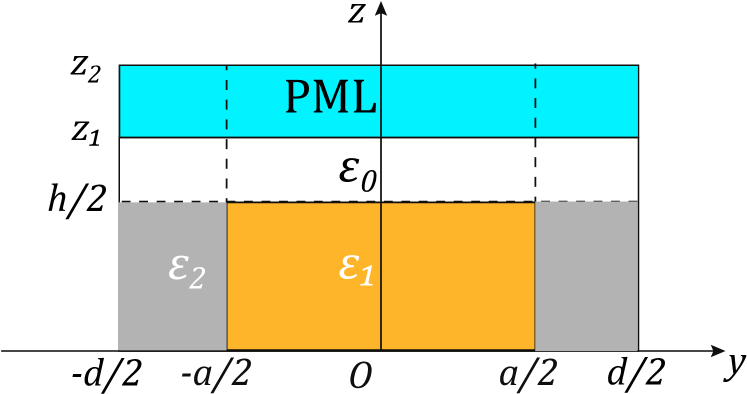
Figure 15: One period of the periodic slab divided into subdomains of constant permittivity.

The PML replaces $z$ by $\hat{z}$ or $dz$ by $d\hat{z}=s(z)\,dz$ for a complex function $s(z)$. Hence, Eq. (15) becomes

$$\frac{1}{s(z)}\frac{\partial}{\partial z}\left[\frac{1}{s(z)}\frac{\partial\phi}{\partial z}\right]+\frac{\partial^{2}\phi}{\partial y^{2}}+2i\beta\frac{\partial\phi}{\partial y}-\beta^{2}\phi=-k^{2}\varepsilon\phi.$$ (16)

In addition, $\phi$ must satisfy the boundary conditions

$$\phi(y,0)=\phi(y,z_{2})=0,$$ (17)

and periodic conditions

$$\phi(-d/2,z)=\phi(d/2,z),$$ (18)

$$\frac{\partial\phi}{\partial y}(-d/2,z)=\frac{\partial\phi}{\partial y}(d/2,z).$$ (19)

We use the Chebyshev pseudospectral method Trefethen (2000) to discretize Eq. (16) on each rectangular subdomain shown in Fig. 15, and impose field continuity conditions and conditions (17)-(19) on the boundaries of the subdomains. The result is a linear matrix eigenvalue problem of the form

$${\bm{L}}{\bm{\phi}}=k^{2}{\bm{\phi}},$$ (20)

where ${\bm{\phi}}$ is a vector containing the values of $\phi$ at the interior Chebyshev collocation points.

The eigenvalue problem for resonant modes on the periodic slab can also be solved by a nonlinear scheme based on the mode matching method. For the odd (in $z$) modes, the structure is divided into two layers given by $0<z<h/2$ and $z>h/2$, and the dielectric function is $\varepsilon^{(1)}(y)$ and $\varepsilon^{(2)}(y)$ in these two layers, respectively. For given $\beta$ and $k$, we can expand $\phi$ in each layer in one-dimensional eigenmodes. The eigenvalue problem in the $l$-th layer is

$$\left[\frac{d^{2}}{dy^{2}}+2i\beta\frac{d}{dy}+k^{2}\varepsilon^{(l)}(y)-\beta^{2}\right]\psi^{(l)}=[\eta^{(l)}]^{2}\psi^{(l)},$$

subject to the periodic boundary conditions

$$\psi^{(l)}(-d/2)=\psi^{(l)}(d/2),$$

$$\frac{d\psi^{(l)}}{dy}(-d/2)=\frac{d\psi^{(1)}}{dy}(d/2).$$

Solving the above by the Chebyshev collocation method Trefethen (2000), we obtain

$$\left\{\psi^{(l)}_{j},\,\eta^{(l)}_{j}\right\}_{j=1}^{N},\quad l=1,2,$$

for a positive integer $N$ and discretization points $\{y_{p}\}_{p=1}^{N}$.

With the above eigenmodes, $\phi$ can be expanded as

$$\phi(y,z)=\sum_{j=1}^{N}\frac{c_{j}\sin(\eta^{(1)}_{j}z)}{\sin(0.5\eta^{(1)}_{j}h)}\psi^{(l)}_{j}(y),\ \ 0\leq z<\frac{h}{2},$$

$$\phi(y,z)=\sum_{j=1}^{N}d_{j}e^{i\eta^{(2)}_{j}(z-h/2)}\psi^{(2)}_{j}(y),\quad z>\frac{h}{2}.$$

Enforcing the continuity of $\phi$ and $\partial_{z}\phi$ at $y=y_{p}$ and $z=h/2$ for $1\leq p\leq N$, we obtain the following linear system

$${\bm{A}}\begin{bmatrix}\mathbf{c}\cr\mathbf{d}\end{bmatrix}=\begin{bmatrix}{\bm{A}}_{11}&{\bm{A}}_{12}\\ {\bm{A}}_{21}&{\bm{A}}_{22}\end{bmatrix}\begin{bmatrix}{\bm{c}}\cr{\bm{d}}\end{bmatrix}={\bm{0}},$$ (21)

where ${\bm{c}}$ and ${\bm{d}}$ are column vectors of $c_{j}$ and $d_{j}$ ($1\leq j\leq N$), respectively, ${\bm{A}}$ is a $2\times 2$ block matrix depending on $\beta$ and $k$, and the $(p,j)$ entries of the matrix blocks are

$${\bm{A}}_{11}(p,j)=\psi^{(1)}_{j}(y_{p}),$$

$${\bm{A}}_{12}(p,j)=-\psi^{(2)}_{j}(y_{p}),$$

$${\bm{A}}_{21}(p,j)=\eta^{(1)}_{j}\cot(0.5\eta^{(1)}_{j}h)\psi^{(1)}_{j}(y_{p}),$$

$${\bm{A}}_{22}(p,j)=-i\eta_{j}^{(2)}\psi^{(2)}_{j}(y_{p}).$$

Equation (21) has a nontrivial solution, only when ${\bm{A}}$ is singular. Therefore, we can find the complex $k$ from the condition $\lambda_{1}({\bm{A}})=0$, where $\lambda_{1}(A)$ is the eigenvalue of ${\bm{A}}$ with the smallest magnitude.

References

- Kato (1966) T. Kato, Perturbation Theory for Linear Operators (Springer, Berlin, 1966).
- Moiseyev (2011) N. Moiseyev, Non-Hermitian Quantum Mechanics (Cambridge University Press, 2011).
- Heiss (2012) W. D. Heiss, “The physics of exceptional points,” J. Phys. A: Math. Theor. 45, 444016 (2012).
- Jones (1988) C. A. Jones, “Multiple eigenvalues and mode classification in plane Poiseuille flow,” Q. J. Mech. Appl. Math. 41, 363–382 (1988).
- Heiss and Sannino (1990) W. D. Heiss and A. L. Sannino, “Avoided level crossing and exceptional points,” J. Phys. A 23, 1167 (1990).
- Heiss and Sannino (1991) W. D. Heiss and A. L. Sannino, “Transitional regions of finite Fermi systems and quantum chaos,” Phys. Rev. A 43, 4159–4166 (1991).
- Leyvraz and Heiss (2005) F. Leyvraz and W. D. Heiss, “Large- scaling behavior of the Lipkin-Meshkov-Glick model,” Phys. Rev. Lett. 95, 050402 (2005).
- Cartarius et al. (2008) H. Cartarius, J. Main, and G. Wunner, “Discovery of exceptional points in the Bose-Einstein condensation of gases with attractive interaction,” Phys. Rev. A 77, 013618 (2008).
- Bender and Boettcher (1998) C. M. Bender and S. Boettcher, “Real spectra in non-Hermitian Hamiltonians having symmetry,” Phys. Rev. Lett. 80, 5243–5246 (1998).
- Bender et al. (1999) C. M. Bender, S. Boettcher, and P. N. Meisinger, “PT-symmetric quantum mechanics,” J. Math. Phys. 40, 2201–2229 (1999).
- Bender et al. (2002) C. M. Bender, M. V. Berry, and A. Mandilara, “Generalized PT symmetry and real spectra,” J. Phys. A: Math. Gen. 35, L467 (2002).
- Klaiman et al. (2008) S. Klaiman, U. Günther, and N. Moiseyev, “Visualization of branch points in -symmetric waveguides,” Phys. Rev. Lett. 101, 080402 (2008).
- Rüter et al. (2010) C. E. Rüter, K. G. Makris, R. El-Ganainy, D. N. Christodoulides, M. Segev, and D. Kip, “Observation of parity-time symmetry in optics,” Nat. Phys. 6, 192 (2010).
- Liertzer et al. (2012) M. Liertzer, L. Ge, A. Cerjan, A. D. Stone, H. E. Türeci, and S. Rotter, “Pump-induced exceptional points in lasers,” Phys. Rev. Lett. 108, 173901 (2012).
- Peng et al. (2014) B. Peng, Ş. K. Özdemir, S. Rotter, H. Yilmaz, M. Liertzer, F. Monifi, C. M. Bender, F. Nori, and L. Yang, “Loss-induced suppression and revival of lasing,” Science 346, 328–332 (2014).
- Brandstetter et al. (2014) M. Brandstetter, M. Liertzer, C. Deutsch, P. Klang, J. Schöberl, H. E. Türeci, G. Strasser, K. Unterrainer, and S. Rotter, “Reversing the pump dependence of a laser at an exceptional point,” Nat. Commun. 5, 4034 (2014).
- Hodaei et al. (2017) H. Hodaei, A. U. Hassan, S. Wittek, H. Garcia-Gracia, R. El-Ganainy, D. N. Christodoulides, and M. Khajavikhan, “Enhanced sensitivity at higher-order exceptional points,” Nature 548, 187 (2017).
- Chen et al. (2017a) W. Chen, S. K. Özdemir, G. Zhao, J. Wiersig, and L. Yang, “Exceptional points enhance sensing in an optical microcavity,” Nature 548, 192 (2017a).
- Goldzak et al. (2018) T. Goldzak, A. A. Mailybaev, and N. Moiseyev, “Light stops at exceptional points,” Phys. Rev. Lett. 120, 013901 (2018).
- Feng et al. (2014) L. Feng, Z. J. Wong, R.-M. Ma, Y. Wang, and X. Zhang, “Single-mode laser by parity-time symmetry breaking,” Science 346, 972–975 (2014).
- Lin et al. (2011) Z. Lin, H. Ramezani, T. Eichelkraut, T. Kottos, H. Cao, and D. N. Christodoulides, “Unidirectional invisibility induced by -symmetric periodic structures,” Phys. Rev. Lett. 106, 213901 (2011).
- Chen et al. (2017b) W. Chen, S. K. Özdemir, G. Zhao, J. Wiersig, and L. Yang, “Exceptional points enhance sensing in an optical microcavity,” Nature 548, 192 (2017b).
- Zhen et al. (2015) B. Zhen, C. W. Hsu, Y. Igarashi, L. Lu, I. Kaminer, A. Pick, S.-L. Chua, J. D. Joannopoulos, and M. Soljacic, “Spawning rings of exceptional points out of Dirac cones,” Nature 525, 35 (2015).
- Kamiński et al. (2017) P. M. Kamiński, A. Taghizadeh, O. Breinbjerg, J. Mørk, and S. Arslanagić, “Control of exceptional points in photonic crystal slabs,” Opt. Lett. 42, 2866–2869 (2017).
- Hsu et al. (2016) C. W. Hsu, B. Zhen, A. D. Stone, J. D. Joannopoulos, and M. Soljacic, “Bound states in the continuum,” Nat. Rev. Mater. 1, 16048 (2016).
- Trefethen (2000) L. N. Trefethen, Spectral Methods in MATLAB (Society for Industrial and Applied Mathematics (SIAM), Philadelphia, PA, 2000).
- Berenger (1994) J. P. Berenger, “A perfectly matched layer for the absorption of electromagnetic waves,” J. Comput. Phys. 114, 185–200 (1994).
- Chew and Weedon (1994) W. C. Chew and W. H. Weedon, “A 3D perfectly matched medium from modified Maxwell’s equations with stretched coordinates,” Microw. Opt. Technol. Lett. 7, 599–604 (1994).