A $C^{0}$ linear finite element method for sixth order elliptic equations

Abstract

In this paper, we develop a straightforward $C^{0}$ linear finite element method for sixth-order elliptic equations. The basic idea is to use gradient recovery techniques to generate higher-order numerical derivatives from a $C^{0}$ linear finite element function. Both theoretical analysis and numerical experiments show that the proposed method has the optimal convergence rate under the energy norm. The method avoids complicated construction of conforming $C^{2}$ finite element basis or nonconforming penalty terms and has a low computational cost.

AMS subject classifications.  Primary 65N30; Secondary 45N08

Key words.  Sixth-order equation, Gradient recovery, Linear finite element.

1 Introduction

Partial differential equations (PDEs) with order higher than 2 have been widely used to describe different physical laws in material sciences [14, 15, 29, 30, 39], elastic mechanics[42], quantum mechanics[24], plasma physics[10, 11, 22], differential geometry [16, 41], and other areas of science and engineering. Comparing with the second-order PDEs, higher order PDEs are much less studied, including some fundamental theoretical issues such as existence, uniqueness, and regularity of solutions.

Numerical simulation becomes an important tool to study high order PDEs, and yet the design of efficient and reliable numerical methods is very challenging. As usual, the finite element method (FEM) plays a critical role in the numerical simulation. Both conforming and nonconforming methods have been applied to solve high order PDEs in the literature. Usually, a conforming method requires higher regularity of the approximating functions (e.g. $C^{1}$ functions for a fourth-order PDE and $C^{2}$ for a sixth-order PDE), while a nonconforming method avoids the construction of higher regularity finite elements by adding some specially designed penalty terms to the scheme. The complicated construction of high regularity finite elements (for conforming methods) or penalty terms (for nonconforming methods) makes these two FEMs hard to be implemented and significantly increases computational cost. Moreover, the analysis of the aforementioned FEMs is often very complicated.

In this work, we present a systematic and simple numerical approach to treat high-order PDEs and shed some light on theoretical analysis for this new method. To be more precise, we will develop a gradient recovery technique based $C^{0}$ linear finite element method for the following sixth-order equation

$$-\triangle^{3}u = f\ \ \ \ {\rm in}\ \Omega$$ (1.1)

$$u=\partial_{\bf n}u=\partial^{2}_{\bf nn}u = 0\ \ \ \ {\rm on}\ \partial\Omega,$$ (1.2)

where $\Omega\subset\mathbb{R}^{2}$ is an open bounded domain, $f\in L^{2}(\Omega)$, ${\bf n}$ is the outward unit normal of the boundary $\partial\Omega$. The sixth order derivative is defined as

$$\Delta^{3}u=\Delta(\Delta(\Delta u))=\sum_{i,j,k=1}^{2}\frac{\partial^{6}u}{\partial x_{i}^{2}\partial x_{j}^{2}\partial x_{k}^{2}}$$

and the directional derivatives are $\partial_{\bf n}u=\nabla u\cdot{\bf n},\partial^{2}_{\bf nn}u={\bf n}^{T}D^{2}u\cdot{\bf n}$. The (weak) solution of (1.1)-(1.2) is a function $u\in H^{3}_{0}(\Omega)$ satisfying

$$a(u,v)=(f,v),\forall v\in H_{0}^{3}(\Omega),$$ (1.3)

where the third order derivative tensor is given by $D^{3}v=\frac{\partial^{3}v}{\partial x_{i}\partial x_{j}\partial x_{k}}$ and the bilinear form is

$$a(v,w)=\int_{\Omega}D^{3}v:D^{3}w,\quad\forall v,w\in H^{3}(\Omega).$$

Here the Frobenius product “:” for two tensors $B_{1}=(b_{ijk}^{1}),B_{2}=(b_{ijk}^{2})$ is defined as

$$B_{1}:B_{2}=\sum_{i,j,k=1}^{2}b^{1}_{ijk}b^{2}_{ijk}.$$

Note that the sixth-order elliptic boundary value problem (1.1) arises from many mathematical models including differential geometry([16, 41]), the thin-film equations [9], and the phase field crystal model [8, 18, 40]. For simplicity, we choose the homogeneous Dirichlet boundary conditions. The basic principle can be applied to other boundary conditions as well.

Let us illustrate the basic idea of the construction of our novel method. Note that the bilinear form $a(\cdot,\cdot)$ involves the third derivative of the discrete solution, which is impossible to obtain from a direct calculation of $C^{0}$ linear element whose gradient is piecewise constant (w.r.t the underlying mesh) and discontinuous across each element. To overcome this difficulty, we use the gradient recovery operator $G_{h}$ to “lift” discontinuous piecewise constant $Dv_{h}$ to continuous piecewise linear function $G_{h}v_{h}$, see [47, 2, 3, 4, 5, 7, comsol08, 20, 45] for the details of different recovery operators. In other words, we use the special difference operator $DG_{h}^{2}$ to discretize the third order differential operator $D^{3}$. Our algorithm is then designed by applying this special difference operator to the standard Ritz-Galerkin method.

From the above construction, our method has some obvious advantages. First, the fact that the recovery operator $G_{h}$ can be defined on a general unstructured grid implies that the method is valid for problems on arbitrary domains and meshes. Second, our method only has function value unknowns on nodal points instead of both function value and derivative unknowns, its computational complexity is much lower than existing conforming and non-conforming methods in the literature.

Naturally, one may question on the consistency, stability, and convergence of the proposed method, which require some more in-depth mathematical analysis. Let us begin with a discussion of consistency. As indicated in [45] (resp. [25]), for reasonably regular meshes, $G_{h}u_{I}$ (resp. $G_{h}^{2}u_{I}$) is a second-order finite difference scheme of the gradient $Du$ (resp. $D^{2}u$), if $u$ is sufficiently smooth. Here $u_{I}$ is the interpolation of $u$ in linear finite element space. As a consequence, $DG_{h}^{2}u_{I}$ is a first-order approximation of $D^{3}u$, provided $u$ is sufficiently smooth. However, for a discrete function $v_{h}$ in the finite element space which is not smooth across the element edges, the error $\|Dv_{h}-G_{h}v_{h}\|_{0}$ is not a small quantity of the high order, sometimes it may not converge to zero at all. Fortunately, an error estimate in [26, 17] set up a consistency in a weak sense, see (3.19) and (3.20) for the details. This weak consistency property of the gradient recovery operator will play an important role in our error analysis.

Next we discuss stability, which in our case can be reduced to verification of the (uniform) coercivity of the bilinear form $(DG_{h}^{2}\cdot,DG_{h}^{2}\cdot)$ in the following sense

$$\|v_{h}\|_{0}\lesssim\|DG_{h}^{2}v_{h}\|_{0},$$ (1.4)

for all $v_{h}$ in the finite element space with suitable boundary conditions. Again, since the discrete Poincaré inequality (3.18) has been established in [26], the stability (1.4) is a direct consequence. Note that (1.4) implies that no additional penalty term is needed in order to guarantee the stability, and this fact makes our method very simple.

The convergence properties of our method depends heavily on the aforementioned consistency, stability, and the nice approximation properties of the recovery operator $G_{h}$. As usual, the analysis of the error between the exact and approximate solutions can be decomposed into the analysis of the approximation error and consistency error. Combining the weak consistency error estimates (3.19),(3.20) and approximation error estimates (3.15)-(3.17) leads to the optimal convergence rate ($=1$) under the energy norm ($H^{3}$ norm). This convergence rate is observed numerically. Furthermore, we also notice a second-order convergence rate under both $H^{1}$ and $L^{2}$ norms. However, we are only able to prove a sub-optimal convergence rate $\frac{3}{2}$ under both the $H^{1}$ and $L^{2}$ norms at this moment. We would like to emphasize that our analysis here is straightforward and simpler than the analysis of traditional conforming and nonconforming methods applied to sixth-order PDEs.

The rest of the paper is organized as follows. We first present our algorithm in Section 2. Several numerical examples are provided in Section 3 to illustrate the efficiency and convergence rates of our algorithm. In Section 4, a rigorous mathematical analysis of our algorithm is given. Finally, some concluding remarks are presented in the final section.

2 A recovery based $C^{0}$ linear FEM

In this section, we discretize the variational equation (1.3) in the standard $C^{0}$ linear finite element space.

Let ${\mathcal{T}}_{h}$ be a triangulation of $\Omega$ with mesh-size $h$. We denote by ${\mathcal{N}}_{h}$ and ${\mathcal{E}}_{h}$ the set of vertices and edges of ${\mathcal{T}}_{h}$, respectively. Let $V_{h}$ be the standard ${\mathcal{P}}_{1}$ finite element space corresponding to ${\mathcal{T}}_{h}$. It is well-known that $V_{h}={\rm Span}\{\phi_{p}:p\in{\mathcal{N}}_{h}\}$ with $\phi_{p}$ a linear nodal basis corresponding to each vertex $p\in{\mathcal{N}}_{h}$. Let $G_{h}:V_{h}{\longrightarrow}{V_{h}\times V_{h}}$ be a gradient recovery operator defined as below ([47, 34]). For each vertex $p\in{\mathcal{N}}_{h}$, we define a recovered derivative $(G_{h}v_{h})(p)$ and let the whole recovered gradient function be

$$G_{h}v_{h}=\sum_{p\in{\mathcal{N}}_{h}}(G_{h}v_{h})(p)\phi_{p}.$$

For all $v_{h}\in V_{h}$, we have $G_{h}v_{h}=(G_{h}^{x_{1}}v_{h},G_{h}^{x_{2}}v_{h})\in{V_{h}\times V_{h}}$. The corresponding recovered Hessian matrix is defined as follows [25]:

$$G_{h}^{2}v_{h}=\left(\begin{array}[]{ll}G_{h}^{x_{1}}G_{h}^{x_{1}}v_{h}&G_{h}^{x_{1}}G_{h}^{x_{2}}v_{h}\\ G_{h}^{x_{2}}G_{h}^{x_{1}}v_{h}&G_{h}^{x_{2}}G_{h}^{x_{2}}v_{h}\end{array}\right).$$

The derivative of $G_{h}^{2}v_{h}$ is a tensor with its component

$$(DG_{h}^{2}v_{h})_{ijk}=\partial_{x_{i}}G_{h}^{x_{j}}G_{h}^{x_{k}}v_{h},i,j,k=1,2.$$

For all $v_{h},w_{h}\in V_{h}$, we define a discrete bilinear form

$$a_{h}(v_{h},w_{h})=\int_{\Omega}D(G_{h}^{2}v_{h}):D(G_{h}^{2}w_{h}),$$

The gradient recovery linear element scheme for solving (1.1) reads as : Find $u_{h}\in V_{h}^{0}$ such that

$$a_{h}(u_{h},v_{h}) = (f,v_{h}),\quad v_{h}\in V_{h}^{0},$$ (2.5)

where the homogenous finite element space

$$V_{h}^{0}=\{v_{h}\in V_{h}|v_{h}=G_{h}v_{h}\cdot{\bf n}=G_{h}v_{h}\cdot{\bf t}={\bf n}^{T}G_{h}^{2}v_{h}{\bf n}=0\ {\rm on}\ \partial\Omega\}.$$

Note that here we use an additional condition $G_{h}v_{h}\cdot{\bf t}=0$ since the exact solution satisfies $\frac{\partial u}{\partial{\bf t}}=0$ on $\partial\Omega$, where ${\bf t}$ is the unit tangential vector on $\partial\Omega$.

Remark 2.1.

For sixth order partial differential equation (1.1)-(1.2), all three boundary conditions are essential boundary conditions and we should incorporate such types boundary conditions into the discretized linear system instead of the weak form. For partial differential equation (1.1) with nonhomogeneous boundary conditions

$$u|_{\partial\Omega}=g_{D},\quad\partial_{\bf n}u|_{\partial\Omega}=g_{N},\quad\partial^{2}_{\bf nn}u|_{\partial\Omega}=g_{R}.$$ (2.6)

The variation form is to find $u_{h}\in V_{h}$ with $u_{h}|_{\partial\Omega}=g_{D},\partial_{\bf n}u_{h}|_{\partial\Omega}=g_{N},\partial^{2}_{\bf nn}u_{h}|_{\partial\Omega}=g_{R}$ such that

$$a_{h}(u_{h},v_{h}) = (f,v_{h}),\quad v_{h}\in V_{h}^{0},$$

For numerical implement, there is no difference between homogeneous and nonhomogeneous boundary conditions. In the article, we suppose homogeneous boundary conditions only for simplifying numerical analysis.

Remark 2.2.

The scheme (2.5) depends on the definition of $(G_{h}v_{h})(p)$ at each vertex $p\in{\mathcal{N}}_{h}$. In the following, three popular definitions of $(G_{h}v_{h})(p)$ are listed (c.f., [47, 34]).

(a) Weighted averaging(WA). For each $p\in{\mathcal{N}}_{h}$, let the element patch $\omega_{p}=\cup\{\tau:p\in\bar{\tau}\}$ and define

$$(G_{h}v_{h})(p)=\frac{1}{|\omega_{p}|}\int_{\omega_{p}}\nabla v_{h}(x_{1},x_{2})dx_{1}dx_{2}.$$ (2.7)

(b) Local $L^{2}$-projection. We seek two polynomials $P_{l}\in{\mathcal{P}}^{1}(\omega_{p}),(l=1,2)$, such that

$$\int_{\omega_{p}}[P_{l}(x_{1},x_{2})-\partial_{x_{l}}v(x_{1},x_{2})]Q(x_{1},x_{2})dx_{1}dx_{2}=0,\quad\forall Q\in\mathcal{P}^{1}(\omega_{p}),l=1,2$$ (2.8)

and we define

$$(G_{h}v_{h})(p)=(P_{1}(p),P_{2}(p)).$$

Sometimes, the exact integral in (2.8) is replaced by its discrete counterpart so that the two polynomials $P_{l},l=1,2$ satisfying the least square fitting equation (SPR)

$$\sum_{i=1}^{m}[P_{l}(x^{i}_{1},x^{i}_{2})-\partial_{x^{i}_{l}}v(x^{i}_{1},x^{i}_{2})]Q(x^{i}_{1},x^{i}_{2})=0,\quad\forall Q\in\mathcal{P}^{1}(\omega_{P}),l=1,2,$$ (2.9)

where $(x_{1}^{i},x_{2}^{i}),i=1,\ldots,m$ are $m$ given points in $\omega_{p}$.

(c) The polynomial preserving recovery (PPR). We seek a quadratic function $P\in\mathcal{P}^{2}(\omega_{p})$, such that

$$\sum_{i=1}^{m}[P(x_{1}^{i},x_{2}^{i})-v(x_{1}^{i},x_{2}^{i})]Q(x_{1}^{i},x_{2}^{i})=0,\quad\forall Q\in\mathcal{P}^{2}(\omega_{P}).$$ (2.10)

Then we can define $(G_{h}v_{h})(p)=(\partial_{x_{1}}P(p),\partial_{x_{2}}P(p))$.

It is known that the above three definitions are equivalent on a mesh of uniform triangular pattern [45].

Remark 2.3.

Essentially, the operator $G_{h}$ can be regarded as a difference operator defined on unstructured grids. This operator lifts discontinuous gradient generated from a $C^{0}$-FEM to a continuous one, and thereby makes the further calculation of high order derivatives possible.

Remark 2.4.

The scheme (2.5) is very simple and straightforward. It avoids the complicated construction of conforming $C^{2}$ finite element basis (c.f., [28]) or the complicated construction of nonconforming penalty terms ([27]).

For $\mathcal{A}\subset\Omega$, let $V_{h}(\mathcal{A})$ denote the restrictions of functions in $V_{h}$ to $\mathcal{A}$ and let $V_{h}^{\text{comp}}(\mathcal{A})$ denote the set of those functions in $V_{h}(\mathcal{A})$ with compact support in the interior of $\mathcal{A}$ [37]. Let $\Omega_{0}\subset\subset\Omega_{1}\subset\subset\Omega_{2}\subset\subset\Omega$ be separated by $d\geq c_{o}h$ and $\ell$ be a direction, i.e., a unit vector in $\mathbb{R}^{2}$. Let $\tau$ be a parameter, which will typically be a multiply of $h$. Let $T^{\ell}_{\tau}$ denote translation by $\tau$ in the direction $\ell$, i.e.,

$$T^{\ell}_{\tau}v(x)=v(x+\tau\ell),$$ (2.11)

and for an integer $\nu$

$$T^{\ell}_{\nu\tau}v(x)=v(x+\nu\tau\ell).$$ (2.12)

Following the definition of [37], the finite element space $V_{h}$ is called translation invariant by $\tau$ in the direction $\ell$ if

$$T^{\ell}_{\nu\tau}v\in V^{\text{comp}}_{h}(\Omega),\quad\forall v\in V^{\text{comp}}_{h}(\Omega_{1}),$$ (2.13)

for some integer $\nu$ with $|\nu|<M$. Equivalently, $\mathcal{T}_{h}$ is called a translation invariant mesh. As illustrated in [25], uniform meshes of regular pattern, chevron pattern, cirsscross patter, and unionjack pattern are all translation invariant.

3 Analysis

The section is dedicated to a mathematical proof for the convergence properties.

To this end, we need some properties of $G_{h}$. For the polynomial preserving recovery operator $G_{h}$, there are the following boundedness property (see (2.11) in [34])

$$\|G_{h}v_{h}\|_{0}\lesssim|v_{h}|_{1},\quad v_{h}\in V_{h}$$ (3.14)

and the superconvergence approximation properties

$$\|\nabla u-G_{h}u_{I}\|_{0}\lesssim h^{2}|u|_{3,\infty}{,}\quad u\in W^{3,\infty}(\Omega).$$ (3.15)

Here $u_{I}$ is the linear interpolation of $u$ in $V_{h}$. In addition, we will utilize the following ultraconvergence approximation properties of Hessian recovery operator (see Theorem 3.5 in [25])

$$\|D^{3}u-DG^{2}_{h}u_{I}\|_{0} \lesssim h|u|_{4,\infty}{,}\quad u\in W^{4,\infty}(\Omega),$$ (3.16)

$$\|D^{2}u-G^{2}_{h}u_{I}\|_{0} \lesssim h^{2}|u|_{4,\infty}{,}\quad u\in W^{4,\infty}(\Omega),$$ (3.17)

provided the mesh $\mathcal{T}_{h}$ is translation invariant.

Remark 3.1.

We would like to comment that the requirement $\mathcal{T}_{h}$ translation invariant for proving approximation properties (3.16) and (3.17) only for theoretical purpose. In practical, our method can be applied to and shows optimal convergence on arbitrary unstructured mesh.

To analyze the convergence of the scheme (2.5), we suppose that the ${\mathcal{T}}_{h}$ is sufficient regular such that there holds the following discrete Poincaré inequality (cf.,[26])

$$\ \ \ \|v_{h}\|_{i}\lesssim\|G_{h}v_{h}\|_{i},\forall v_{h}\in V_{h}^{0},i=0,1$$ (3.18)

and discrete weak approximation properties

$$\left|\int_{\Omega}\nabla v\cdot(G_{h}v_{h}-\nabla v_{h})\right| \lesssim h\|v\|_{2}|G_{h}v_{h}|_{1},\forall v\in H^{2},$$ (3.19)

$$\left|\int_{\Omega}\nabla v\cdot(G_{h}v_{h}-\nabla v_{h})\right| \lesssim h^{2}\|v\|_{3}|G_{h}v_{h}|_{1},\forall v\in H^{3}.$$ (3.20)

Note that both (3.18) and (3.19) have been discussed in the analysis of a recovery operator based linear finite element method for the biharmonic equation by Guo et al. in [26]. In their paper, a counter-example shows that the strong error $\|\nabla v_{h}-G_{h}v_{h}\|_{0}$ is not necessary of ${\mathcal{O}}(h)$ for all $v_{h}\in V_{h}$ (which means the weak estimate (3.19) might be the best estimate of the difference $\nabla v_{h}-G_{h}v_{h}$).

By (3.18), for all $v_{h}\in V_{h}^{0}$, we have

$$\|v_{h}\|_{0}\lesssim\|G_{h}v_{h}\|_{0}\lesssim\|G_{h}^{2}v_{h}\|_{0}\lesssim\|DG_{h}^{2}v_{h}\|_{0}.$$

In other words, the semi-norm $\|DG_{h}^{2}\cdot\|_{0}$ is a norm. Then by the Lax-Milgram theorem, the scheme (2.5) has a unique solution . Moreover, by (2.5),

$$\|DG_{h}^{2}u_{h}\|_{0}^{2}=a_{h}(u_{h},u_{h})=(f,u_{h})\lesssim\|f\|_{0}\|v_{h}\|_{0}.$$

Then

$$\|DG_{h}^{2}u_{h}\|_{0}\lesssim\|f\|_{0}$$ (3.21)

which implies the stability of our scheme.

3.1 $H^{3}$ error estimate

Theorem 1.

Let $u_{h}$ be the solution of (2.5) and $u\in H^{6}$ the solution of (1.3). If the mesh ${\mathcal{T}}_{h}$ is translation invariant, $G_{h}$ is properly defined such that (3.14)-(3.20) hold, then

$$\|DG_{h}^{2}(u_{h}-u_{I})\|_{0}\lesssim h\|u\|_{6},$$ (3.22)

where $u_{I}$ is the linear interpolation of $u$ in $V_{h}$. Consequently,

$$\|D^{3}u-DG_{h}^{2}u_{h}\|_{0}\lesssim h\|u\|_{6}.$$ (3.23)

Proof.

Since a weak solution of (1.3) which has regularity $u\in H^{6}$ is also the strong solution satisfying (1.1) and $u_{h}$ is a discrete solution satisfying (2.5), we have

$$a_{h}(u_{h},v_{h})=(f,v_{h})=(-\Delta^{3}u,v_{h}),\forall v_{h}\in V_{h}^{0}.$$

Using the fact that $v_{h}\in V_{h}^{0}$, we have

$$(-\Delta^{3}u,v_{h})=(-(\nabla\cdot\nabla)(\Delta^{2}u),v_{h})=(\nabla(\Delta^{2}u),\nabla v_{h}).$$

Therefore,

$$a_{h}(u_{h},v_{h})=I_{1}+(\nabla(\Delta^{2}u),G_{h}v_{h}),$$

with

$$I_{1}=(\nabla(\Delta^{2}u),\nabla v_{h}-G_{h}v_{h}).$$ (3.24)

Now we deal with the term $(\nabla(\Delta^{2}u),G_{h}v_{h})$. Since $G_{h}v_{h}\cdot{\bf n}=G_{h}v_{h}\cdot{\bf t}=0$ on the boundary $\partial\Omega$, we have that on $\partial\Omega$,

$$\frac{\partial\Delta u}{\partial{\bf n}}\cdot G_{h}v_{h}=\frac{\partial^{2}\Delta u}{\partial{\bf n}\partial{\bf t}}(G_{h}v_{h}\cdot{\bf t})+\frac{\partial^{2}\Delta u}{\partial{\bf n}^{2}}(G_{h}v_{h}\cdot{\bf n})=0.$$

Then

$$(\nabla(\Delta^{2}u),G_{h}v_{h}) = ((\nabla\cdot\nabla)(\Delta(\nabla u)),G_{h}v_{h})$$

$$= -(D^{2}(\Delta u),DG_{h}v_{h}):=-\int_{\Omega}D^{2}(\Delta u):DG_{h}v_{h}.$$

Consequently,

$$(\nabla(\Delta^{2}u),G_{h}v_{h})=I_{2}-(D^{2}(\Delta u),G_{h}^{2}v_{h}),$$

with

$$I_{2}=(D^{2}(\Delta u),G_{h}^{2}v_{h}-DG_{h}v_{h}).$$ (3.25)

Finally, we deal with the term $-(D^{2}(\Delta u),G_{h}^{2}v_{h})$. Writing the gradient as

$$\nabla u=\frac{\partial u}{\partial{\bf n}}{\bf n}+\frac{\partial u}{\partial{\bf t}}{\bf t},$$

we have

$$D^{2}u=\frac{\partial^{2}u}{\partial{\bf n}^{2}}{\bf n}{\bf n}^{T}+\frac{\partial^{2}u}{\partial{\bf t}^{2}}{\bf t}{\bf t}^{T}+\frac{\partial^{2}u}{\partial{\bf n}\partial{\bf t}}({\bf n}{\bf t}^{T}+{\bf t}{\bf n}^{T}),$$

and consequently,

$$\frac{\partial D^{2}u}{\partial{\bf n}}=\frac{\partial^{3}u}{\partial{\bf n}^{3}}{\bf n}{\bf n}^{T}+\frac{\partial^{3}u}{\partial{\bf n}\partial{\bf t}^{2}}{\bf t}{\bf t}^{T}+\frac{\partial^{3}u}{\partial{\bf n}^{2}\partial{\bf t}}({\bf n}{\bf t}^{T}+{\bf t}{\bf n}^{T}).$$

Noting that $u=\frac{\partial u}{\partial{\bf n}}=\frac{\partial^{2}u}{\partial{\bf n^{2}}}=0$ on $\partial\Omega$, we have

$$\frac{\partial^{3}u}{\partial{\bf n}\partial{\bf t}^{2}}=\frac{\partial^{3}u}{\partial{\bf n}^{2}\partial{\bf t}}=0\ {\rm on}\ \Omega.$$

Therefore, on $\partial\Omega$,

$$\frac{\partial D^{2}u}{\partial{\bf n}}:G_{h}^{2}v_{h}=\frac{\partial^{3}u}{\partial{\bf n}^{3}}{\bf n}{\bf n}^{T}:G_{h}^{2}v_{h}=\frac{\partial^{3}u}{\partial{\bf n}^{3}}{\bf n}^{T}G_{h}^{2}v_{h}{\bf n}=0,$$

where in the last equality, we used the fact that ${\bf n}^{T}G_{h}^{2}v_{h}{\bf n}=0$. By Green’s formulas, we finally obtain

$$-(D^{2}(\Delta u),G_{h}^{2}v_{h})=-(\Delta(D^{2}u),G_{h}^{2}v_{h})=(D^{3}u,DG_{h}^{2}v_{h}).$$

In summary, by letting

$$I_{3}=(D^{3}u-DG_{h}^{2}u_{I},DG_{h}^{2}v_{h}),$$

we obtain

$$a_{h}(u_{h}-u_{I},v_{h})=I_{1}+I_{2}+I_{3}.$$ (3.26)

Next, we estimate $I_{i}$ (i = 1, 2, 3) term by term. By (3.18) and (3.19), we have

$$|I_{1}|\lesssim h\|u\|_{6}|G_{h}v_{h}|_{1}\lesssim h||u||_{6}||DG_{h}^{2}v_{h}||_{0}.$$

Similarly, by (3.16),

$$|I_{3}|\lesssim h|u|_{4,\infty}||DG_{h}^{2}v_{h}||_{0}\lesssim h\|u\|_{6}||DG_{h}^{2}v_{h}||_{0}.$$

On the other hand, (3.20) implies

$$|I_{2}|\lesssim h\|u\|_{6}||DG_{h}^{2}v_{h}||_{0}.$$

In a conclusion, we obtain that

$$|a_{h}(u_{h}-u_{I},v_{h})|\lesssim h\|u\|_{6}\|DG_{h}^{2}v_{h}\|_{0},\forall v_{h}\in V_{h}^{0}.$$

Choosing $v_{h}=u_{h}-u_{I}$ in the above estimate, we have (3.22).

The estimate (3.23) is a direct consequence of (3.22) and (3.16), together with the triangle inequality. ∎

3.2 $H^{1}$ error estimate

In this section, we use the Aubin-Nitsche technique to estimate the $H^{1}$ norm error $\|\nabla u-G_{h}u_{h}\|_{0}$. To this end, we construct the following auxiliary problems :

• Find $U\in H_{0}^{3}(\Omega)$ such that

  $$\int_{\Omega}D^{3}U:D^{3}v=(G_{h}(u_{h}-u_{I}),\nabla v),\forall v\in H_{0}^{3}(\Omega).$$ (3.27)

• Find $U_{h}\in V_{h}^{0}$ such that

  $$a_{h}(U_{h},v_{h})=(G_{h}(u_{h}-u_{I}),\nabla v_{h}),\forall v_{h}\in V_{h}^{0}.$$ (3.28)

It is easy to deduce from (3.27) that

$$\|U\|_{5}\lesssim\|G_{h}(u_{h}-u_{I})\|_{0},$$ (3.29)

and from (3.28),(3.18) that

$$\|D(G_{h}^{2}U_{h})\|_{0}\lesssim\|G_{h}(u_{h}-u_{I})\|_{0}.$$ (3.30)

Theorem 2.

Let $u_{h}$ be the solution of (2.5) and $u\in H^{6}$ the solution of (1.3). If the mesh ${\mathcal{T}}_{h}$ is translation invariant, and $G_{h}$ is properly defined such that (3.14)-(3.20) hold, then

$$\|G_{h}(u_{h}-u_{I})\|_{0}\lesssim h^{\frac{3}{2}}\|u\|_{6}.$$ (3.31)

Consequently,

$$\|\nabla u-G_{h}u_{h}\|_{0}\lesssim h^{\frac{3}{2}}\|u\|_{6}.$$ (3.32)

Proof.

First, by the definition of the auxiliary problems, we have

$$(G_{h}(u_{h}-u_{I}),\nabla(u_{h}-u_{I})) = a_{h}(U_{h},u_{h}-u_{I})$$

$$= a_{h}(u_{h}-u_{I},U_{h})$$

$$= (f,U_{h})-a_{h}(u_{I},U_{h})$$

$$= (-\triangle^{3}u,U_{h})-a_{h}(u_{I},U_{h}).$$

Using the same splitting techniques in the previous theorem, we can write

$$(G_{h}(u_{h}-u_{I}),\nabla(u_{h}-u_{I}))=J_{1}+J_{2}+J_{3}+J_{4},$$

where

$$J_{1} = (\nabla(\triangle^{2}u),\nabla U_{h}-G_{h}U_{h}),$$

$$J_{2} = (D^{2}(\triangle u),G_{h}^{2}U_{h}-DG_{h}U_{h}),$$

$$J_{3} = (D^{3}u-DG_{h}^{2}u_{I},D^{3}U),$$

$$J_{4} = (D^{3}u-DG_{h}^{2}u_{I},DG_{h}^{2}U_{h}-D^{3}U).$$

We first estimate $J_{1}$ and $J_{3}$. By (3.20),

$$|J_{1}| \lesssim h^{2}\|u\|_{6}\|DG_{h}U_{h}\|_{0}$$

$$\lesssim h^{2}\|u\|_{6}\|DG_{h}^{2}U_{h}\|_{0}$$

$$\lesssim h^{2}\|u\|_{6}\|G_{h}(u_{h}-u_{I})\|_{0}.$$

and

$$|J_{2}| \lesssim h^{2}\|u\|_{6}\|DG_{h}^{2}U_{h}\|_{0}$$

$$\lesssim h^{2}\|u\|_{6}\|G_{h}(u_{h}-u_{I})\|_{0}.$$

Moreover, using the integration by parts,

$$|J_{3}| \leq \|D^{2}u-G_{h}^{2}u_{I}\|_{0}\|D^{4}U\|_{0}$$

$$\lesssim h^{2}\|u\|_{6}\|G_{h}(u_{h}-u_{I})\|_{0}.$$

Finally, by Cauchy-Schwartz inequality,

$$|J_{4}| \lesssim h^{2}\|u\|_{6}\|U\|_{6}$$

$$\lesssim h^{2}\|u\|_{6}\|G_{h}(u_{h}-u_{I})\|_{1}\lesssim h^{3}\|u\|_{6}^{2}.$$

Summarizing all the above estimates, we obtain

$$(G_{h}(u_{h}-u_{I}),\nabla(u_{h}-u_{I}))\lesssim h^{2}\|u\|_{6}\|G_{h}(u_{h}-u_{I})\|_{0}+h^{3}\|u\|_{6}^{2}.$$

Noticing that

$$\|G_{h}(u_{h}-u_{I})\|_{0}^{2}\sim(G_{h}(u_{h}-u_{I}),\nabla(u_{h}-u_{I})),$$

we arrive that

$$\|G_{h}(u_{h}-u_{I})\|_{0}^{2}\lesssim h^{2}\|u\|_{6}\|G_{h}(u_{h}-u_{I})\|_{0}+h^{3}\|u\|_{6}^{2}.$$

Then the estimate (3.31) follows.

The $H^{1}$ error estimate of (3.32) is a direct consequence of (3.31) and (3.15). ∎

3.3 $L^{2}$ error estimate

Theorem 3.

Let $u_{h}$ be the solution of (2.5) and $u\in H^{6}$ the solution of (1.3). If the mesh ${\mathcal{T}}_{h}$ is sufficiently regular and uniform, $G_{h}$ is properly defined such that (3.14)-(3.20) hold, then

$$\|u-u_{h}\|_{0}\lesssim h^{\frac{3}{2}}\|u\|_{6}.$$ (3.33)

Proof.

By (3.18),

$$\|u_{I}-u_{h}\|_{0} \lesssim \|G_{h}(u_{I}-u_{h})\|_{0}\lesssim h^{\frac{3}{2}}\|u\|_{6}.$$

Then

$$\|u-u_{h}\|_{0} \lesssim \|u-u_{I}\|_{0}+\|u_{I}-u_{h}\|_{0}\lesssim h^{\frac{3}{2}}\|u\|_{6}.$$

∎

Remark 3.2.

In the second section, we observed the convergence rates ${\mathcal{O}}(h^{2})$ both for the errors $\|u-u_{h}\|_{0}$ and $\|\nabla u-G_{h}u_{h}\|_{0}$. However, we can only prove the order ${\mathcal{O}}(h^{3\over 2})$ from our analysis. Further analysis to the scheme is desired to prove the optimal convergence rates of $\|u-u_{h}\|_{0}$ and $\|\nabla u-G_{h}u_{h}\|_{0}$.

4 Numerical Experiments

In this section, we present several numerical experiments to show the convergence rates and efficiency of our method. In all our numerical experiments, $G_{h}$ is chosen as the polynomial preserving recovery operator [46]. To present our numerical results, the following notations are used :

$$De := \|u-u_{h}\|_{0},\quad\quad\quad D^{1}e:=\|\nabla u-\nabla u_{h}\|_{0},$$

$$D^{1}_{r}e := \|\nabla u-G_{h}u_{h}\|_{0},\quad D^{2}e:=\|D^{2}u-DG_{h}u_{h}\|_{0},$$

$$D^{3}e := \|D^{3}u-DG_{h}^{2}u_{h}\|_{0}.$$

Moreover, the convergence rates are listed with respect to the degree of freedom(Dof). Noticing $\text{Dof}\approx h^{-2}$ for a two dimensional grid, the corresponding convergent rates with respect to the mesh size $h$ are double of what we present in the tables 3.1-3.11.

Example 1. We consider the triharmonic problem

$$\left\{\begin{array}[]{ll}-\Delta^{3}u=f&\text{in }\Omega=(0,1)\times(0,1);\\ u=\partial_{\bf n}u=\partial^{2}_{\bf nn}u=0&\text{on }\partial\Omega,\end{array}\right.$$ (4.34)

where $f$ is chosen to fit the exact solution $u(x_{1},x_{2})=x_{1}^{3}(1-x_{1})^{3}x_{2}^{3}(1-x_{2})^{3}$.

First, we apply our scheme (2.5) on regular pattern uniform triangular mesh. The corresponding numerical results are listed in Table 1. It shows that numerical solution $u_{h}$ converges to the exact solution $u$ at a rate of $O(h)$ in recovered $H^{3}$ norm. Also from this table, we observe that $De$ and $D^{1}_{r}e$ converge at a rate of $O(h^{2})$ while $D^{1}e$ and $D^{2}e$ converge at a rate of $O(h)$. Note that convergence rate of $De$ and $D^{1}_{r}e$ is better than that proved in Theorems 2 and 3.

Table 1: Numerical Results Of Example 1 On Regular Pattern Uniform Mesh

Dof	$De$	order	$D^{1}e$	order	$D^{1}_{r}e$	order	$D^{2}e$	order	$D^{3}e$	order
1089	5.61e-06	–	5.76e-05	–	2.57e-05	–	4.01e-04	–	4.46e-03	–
4225	1.54e-06	0.95	2.20e-05	0.71	7.03e-06	0.96	1.73e-04	0.62	2.06e-03	0.57
16641	3.99e-07	0.99	9.65e-06	0.60	1.83e-06	0.98	8.18e-05	0.54	9.99e-04	0.53
66049	1.01e-07	0.99	4.62e-06	0.53	4.66e-07	0.99	4.03e-05	0.51	4.93e-04	0.51

Secondly, we test our scheme on uniform triangular meshes of other patterns, including the chevron, Criss-cross, and Union-Jack patterns. Numerical data are listed in 2, Table 3, and Table 4, respectively. Again, we observed $O(h^{2})$ for $De$, $O(h)$ for $D^{1}e$, $O(h^{2})$ for $D^{1}_{r}e$, $O(h)$ for $D^{2}e$, and $O(h)$ for $D^{3}e$, the same as the regular pattern.

Table 2: Numerical Results Of Example 1 On Chevron Pattern Uniform Mesh

Dof	$De$	order	$D^{1}e$	order	$D^{1}_{r}e$	order	$D^{2}e$	order	$D^{3}e$	order
1089	4.48e-06	–	6.00e-05	–	2.02e-05	–	3.81e-04	–	4.26e-03	–
4225	1.25e-06	0.94	2.22e-05	0.73	5.65e-06	0.94	1.69e-04	0.60	2.04e-03	0.54
16641	3.24e-07	0.99	9.67e-06	0.61	1.47e-06	0.98	8.14e-05	0.53	9.97e-04	0.52
66049	8.24e-08	0.99	4.62e-06	0.54	3.75e-07	0.99	4.03e-05	0.51	4.92e-04	0.51

Table 3: Numerical Results Of Example 1 On Criss-cross Pattern Uniform Mesh

Dof	$De$	order	$D^{1}e$	order	$D^{1}_{r}e$	order	$D^{2}e$	order	$D^{3}e$	order
2113	1.50e-05	–	2.91e-03	–	3.13e-05	–	3.61e-03	–	7.21e-03	–
8321	3.83e-06	1.00	1.48e-03	0.50	8.02e-06	0.99	1.83e-03	0.50	3.62e-03	0.50
33025	9.46e-07	1.01	7.20e-04	0.52	2.02e-06	1.00	8.98e-04	0.52	1.81e-03	0.50
131585	2.39e-07	0.99	3.64e-04	0.49	5.09e-07	1.00	4.55e-04	0.49	9.07e-04	0.50

Table 4: Numerical Results Of Example 1 On Unionjack Pattern Uniform Mesh

Dof	$De$	order	$D^{1}e$	order	$D^{1}_{r}e$	order	$D^{2}e$	order	$D^{3}e$	order
1089	2.61e-05	–	3.24e-03	–	6.30e-05	–	4.33e-03	–	9.40e-03	–
4225	6.53e-06	1.02	1.61e-03	0.51	1.59e-05	1.02	2.12e-03	0.53	4.52e-03	0.54
16641	1.63e-06	1.01	8.03e-04	0.51	4.00e-06	1.01	1.06e-03	0.51	2.22e-03	0.52
66049	4.08e-07	1.01	4.01e-04	0.50	1.00e-06	1.00	5.26e-04	0.50	1.10e-03	0.51

Finally, we turn to the Delaunay mesh. The first level coarse mesh is generated by EasyMesh [23] followed by three levels of regular refinement. Table 5 presents the convergence history for the five different errors. $O(h^{2})$ and $O(h)$ convergence rates are observed for $L_{2}$ and $H_{1}$ errors. As for the $L_{2}$ error of recovered gradient, $O(h^{2})$ superconvergence is observed. Regarding recovered $H_{2}$ and $H_{3}$ errors, $O(h)$ convergence are observed .

In summary, we see that our method converges with optimal rates on all four tested uniform meshes as well as the Delaunay mesh.

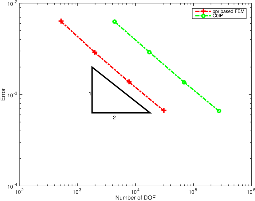
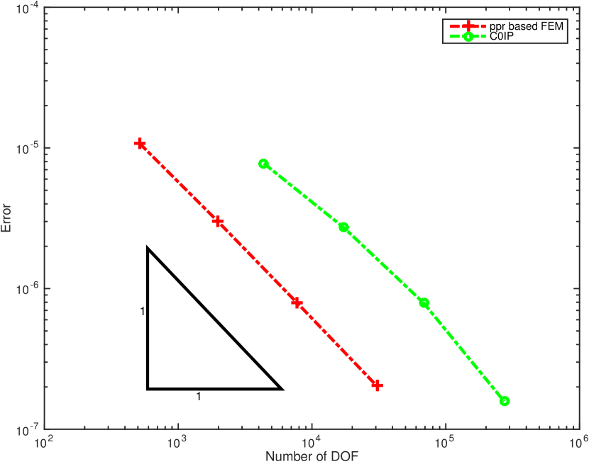
To show the efficiency of our method, we make some numerical comparison with the cubic $C^{0}$ interior penalty method [27] on the same Delaunay meshes. Table 6 shows numerical results of the $C^{0}$ interior penalty method in the $L_{2}$ norm and the energy norm defined in [27]. Consisting with the theoretical result established in [27], the error in the energy norm converges linearly and the $L_{2}$ error decays at rate $O(h^{2})$.

Figures 2 and 2 depict convergent rates of these two methods(i.e. our method and the $C^{0}$ interior penalty method) under the discrete $H_{3}$ (the energy) and $L_{2}$ norms. The rates are almost the same. However, to achieve the same accuracy, our algorithm uses about one-eighth degrees of freedom of the $C^{0}$ interior penalty method.

Table 5: Numerical Results of Example 1 on Delaunay Triangulation with Regular Refinement

Dof	$De$	order	$D^{1}e$	order	$D^{1}_{r}e$	order	$D^{2}e$	order	$D^{3}e$	order
513	1.08e-05	–	9.72e-05	–	4.93e-05	–	6.21e-04	–	6.34e-03	–
1969	3.02e-06	0.95	3.04e-05	0.86	1.38e-05	0.95	2.41e-04	0.70	2.90e-03	0.58
7713	7.94e-07	0.98	1.23e-05	0.66	3.65e-06	0.97	1.08e-04	0.59	1.37e-03	0.55
30529	2.03e-07	0.99	5.77e-06	0.55	9.35e-07	0.99	5.20e-05	0.53	6.67e-04	0.52

Table 6: $C^{0}$ Interior Penalty Method for Example 1 on Delaunay Triangulation with Regular Refinement

Dof	$De$	order	$D^{3}_{h}e$	order
4369	7.75e-06	–	6.25e-03	–
17233	2.72e-06	0.76	2.92e-03	0.55
68449	7.89e-07	0.90	1.37e-03	0.55
272833	1.58e-07	1.16	6.63e-04	0.52

Fig. 1: Comparison of Discrete $H_{3}$ Errors for Example 1

Fig. 2: Comparison of Discrete $L_{2}$ Errors for Example 1

Example 2. In the second example, we will show that our scheme works well also for problems nonhomogeneous boundary conditions. We consider the equation

$$-\Delta^{3}u=\sin(2\pi x_{1})\cos(2\pi x_{2}),(x_{1},x_{2})\in[0,1]^{2}$$

whose exact solution is

$$u(x_{1},x_{2})=\frac{1}{512\pi^{6}}\sin(2\pi x_{1})\cos(2\pi x_{2}),$$

It provides nonhomogeneous boundary conditions $u|_{\partial\Omega},\partial_{\bf n}u|_{\partial\Omega},\partial^{2}_{\bf nn}u|_{\partial\Omega}$.

As in Example 1, we first test our algorithm on regular pattern uniform triangular mesh and list the numerical results in Table 7. Again, $D^{3}e$ decays at rate $O(h)$.As expected, both $De$ and $D^{1}_{r}e$ converges with order $O(h^{2})$. Astonishingly, both $D^{1}e$ and $D^{2}e$ also converge quadratically. Namely, for this example, both $D^{1}e$ and $D^{2}e$ superconverge.

Table 7: Numerical Results Of Example 2 On Regular Pattern Uniform Mesh

Dof	$De$	order	$D^{1}e$	order	$D^{1}_{r}e$	order	$D^{2}e$	order	$D^{3}e$	order
1089	2.50e-07	–	3.21e-05	–	1.53e-06	–	1.35e-04	–	2.25e-03	–
4225	2.66e-08	1.65	7.09e-06	1.11	1.47e-07	1.73	2.93e-05	1.13	7.65e-04	0.80
16641	3.01e-09	1.59	1.46e-06	1.15	1.92e-08	1.48	6.75e-06	1.07	3.24e-04	0.63
66049	4.75e-10	1.34	3.32e-07	1.08	3.41e-09	1.25	1.76e-06	0.98	1.37e-04	0.62

We then consider chevron pattern uniform triangular mesh. Table 8 clearly indicates that $u_{h}$ converges to $u$ at a rate of $O(h^{2})$ under the $L^{2}$ norm, at a rate of $O(h)$ under the $H^{1}$ norm and the recovered $H^{2}$ and $H^{3}$ norms. Moreover, the recovery gradient $G_{h}u_{h}$ converges to $\nabla u$ at a rate of $O(h^{2})$. We also test our algorithms on Delaunay meshes as in the previous example. The numerical data are demonstrated in Table 9. Similar to what we observed in Chevron pattern uniform triangular mesh, the computed error by our method converges to 0 with optimal rates under various norms.

In addition, we have tested our algorithms on other two types (Criss-cross and Union-Jack pattern) uniform triangular meshes. Since the numerical results are similar to the corresponding parts in the previous example, they are not reported here.

Table 8: Numerical Results of Example 2 on Chevron Pattern Uniform Mesh

Dof	$De$	order	$D^{1}e$	order	$D^{1}_{r}e$	order	$D^{2}e$	order	$D^{3}e$	order
1089	4.39e-08	–	1.08e-06	–	4.20e-07	–	1.23e-05	–	2.70e-04	–
4225	3.38e-09	1.89	4.47e-07	0.65	3.92e-08	1.75	3.65e-06	0.90	9.95e-05	0.74
16641	7.89e-10	1.06	2.22e-07	0.51	7.57e-09	1.20	1.61e-06	0.60	4.13e-05	0.64
66049	2.00e-10	1.00	1.11e-07	0.50	1.83e-09	1.03	7.84e-07	0.52	1.78e-05	0.61

Table 9: Numerical Results of Example 2 on Delaunay Triangulation with Regular Refinement

Dof	$De$	order	$D^{1}e$	order	$D^{1}_{r}e$	order	$D^{2}e$	order	$D^{3}e$	order
513	5.52e-08	–	1.77e-06	–	3.81e-07	–	1.29e-05	–	1.44e-04	–
1969	1.17e-08	1.15	5.43e-07	0.88	8.07e-08	1.15	4.21e-06	0.83	5.78e-05	0.68
7713	2.79e-09	1.05	2.57e-07	0.55	1.97e-08	1.03	1.90e-06	0.58	1.94e-05	0.80
30529	6.86e-10	1.02	1.27e-07	0.51	4.91e-09	1.01	9.40e-07	0.51	8.52e-06	0.60

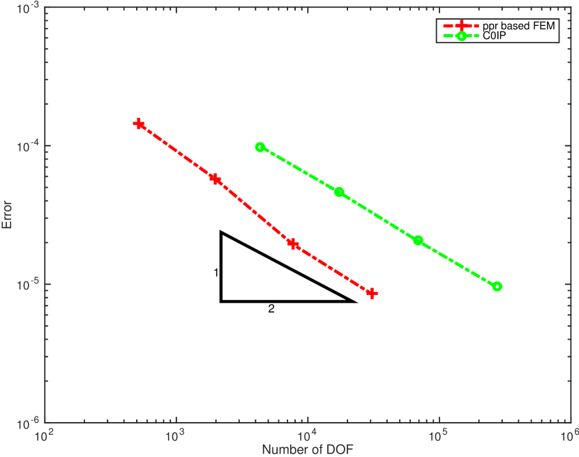
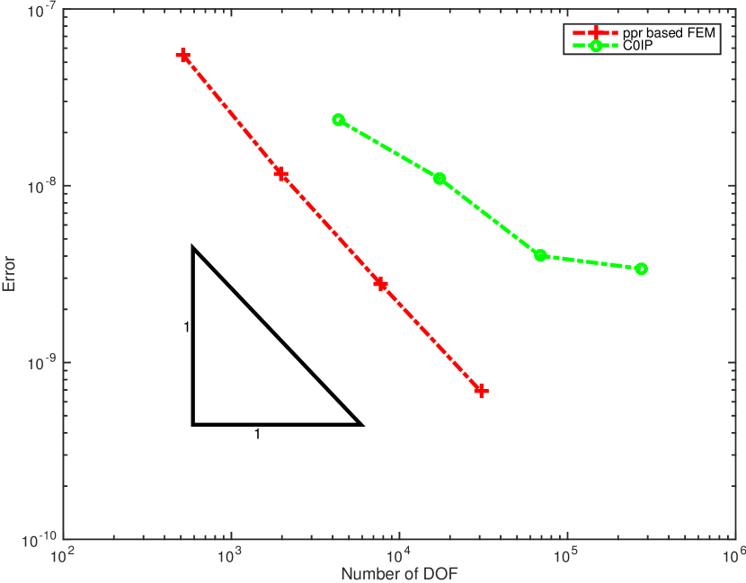
Once again, we present a numerical comparison with the $C^{0}$ interior penalty method. We see from Figure 4 that the convergence rates of $H_{3}$ error are comparable, however, our method requires much less degrees of freedom in order to achieve the same accuracy. Figure 4 indicates that our method is slightly better than the $C^{0}$ interior penalty method with regard to the $L_{2}$ norm which is suboptimal. Here we would like to point out that the error of the $C^{0}$ interior penalty method is sensitive to the penalty parameter.

Fig. 3: Comparison of Discrete $H_{3}$ Errors for Example 2

Fig. 4: Comparison of Discrete $L_{2}$ Errors for Example 2

Example 3. In previous two examples, we consider sixth order elliptic equations on the unit square. To show the ability of dealing arbitrary complex domain, we consider the following sixth order partial differential equation

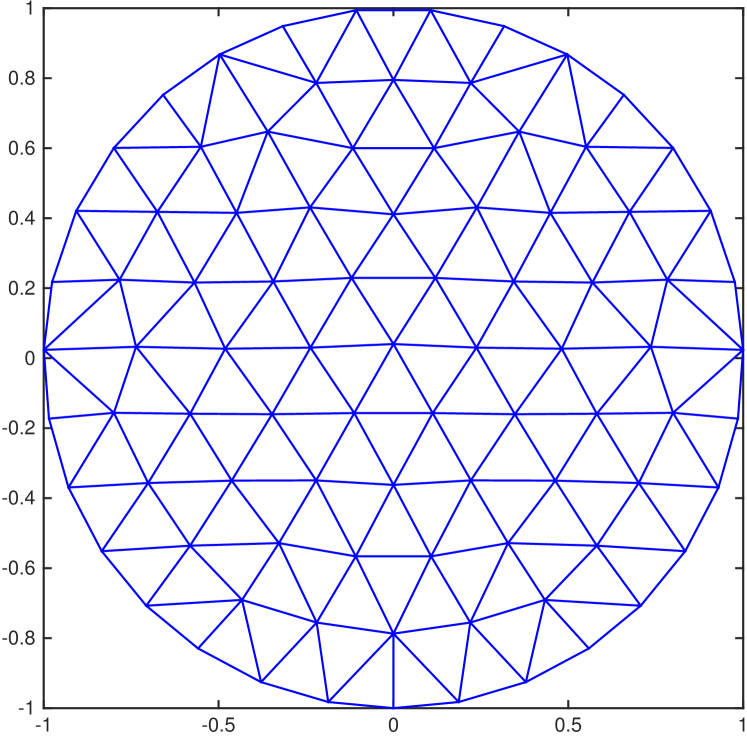
$$-\Delta^{3}u=8e^{x_{1}+x_{2}}.$$

on the unit disk, i.e. $\Omega=\{(x_{1},x_{2})\in\mathbb{R}^{2}:x_{1}^{2}+x_{2}^{2}\leq 1\}$. The exact solution is

$$u(x_{1},x_{2})=e^{x_{1}+x_{2}}.$$

and the corresponding boundary conditions are given by the exact solution. The initial mesh is generated by DistMesh [36] as shown in Figure 6. The other seven level meshes are obtained by refining the initial mesh using regular refinement. The numerical results are reported in Table 10. As in two previous examples, $O(h)$ convergence for $D^{3}e$ , $D^{2}e$, and $D^{1}e$ are observed and $O(h^{2})$ convergence order are observed for $De$ and $D^{1}_{r}e$.

Fig. 5: Initial Mesh On The Unit Disk

Fig. 6: Initial Mesh On The Lshape Domain

Table 10: Numerical Results of Sixth Order PDE in the Unit Disk

Dof	$De$	order	$D^{1}e$	order	$D^{1}_{r}e$	order	$D^{2}e$	order	$D^{3}e$	order
88	3.69e-02	–	4.76e-01	–	1.38e-01	–	1.01e+00	–	3.70e+00	–
318	1.44e-02	0.73	1.91e-01	0.71	3.21e-02	1.14	3.48e-01	0.83	1.92e+00	0.51
1207	1.84e-03	1.54	8.05e-02	0.65	4.76e-03	1.43	1.06e-01	0.89	7.14e-01	0.74
4701	4.16e-04	1.09	4.00e-02	0.51	1.20e-03	1.01	4.94e-02	0.56	3.66e-01	0.49
18553	1.04e-04	1.01	2.00e-02	0.51	3.03e-04	1.00	2.40e-02	0.52	1.99e-01	0.44
73713	2.60e-05	1.00	1.00e-02	0.50	7.57e-05	1.01	1.19e-02	0.51	9.70e-02	0.52
293857	7.01e-06	0.95	5.00e-03	0.50	1.85e-05	1.02	5.94e-03	0.50	4.62e-02	0.54

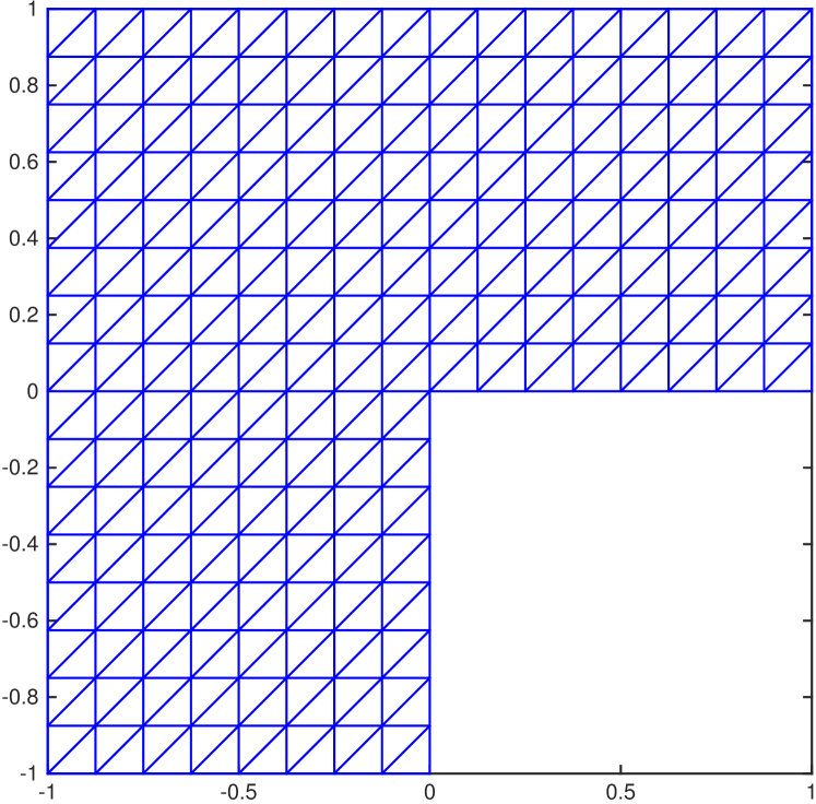
Example 4. As in [28], we consider the following triharmonic equation

$$-\Delta^{3}u=0.$$

on the L-shaped domain $[-1,1]^{2}\setminus([0,1]\times[-1,0])$ with boundary conditions such that the problem has the exact solution

$$u(x_{1},x_{2})=x_{1}^{6}-x_{2}^{6}.$$

Here we use uniform meshes. The initial mesh is plotted in Figure 6, while our numerical results are listed in Table 11. As pointed out in [28], the solution $u$ varies fast near the boundary. Even in that case, we observe the optimal convergence rates under all the norms.

Table 11: Numerical Results For Triharmonic Equation On LShape Domain

Dof	$De$	order	$D^{1}e$	order	$D^{1}_{r}e$	order	$D^{2}e$	order	$D^{3}e$	order
225	2.04e-01	–	5.78e+00	–	8.10e-01	–	1.42e+01	–	7.58e+01	–
833	2.63e-02	1.56	1.69e+00	0.94	1.24e-01	1.43	4.12e+00	0.95	2.96e+01	0.72
3201	3.54e-03	1.49	4.20e-01	1.03	2.70e-02	1.14	1.42e+00	0.79	1.35e+01	0.58
12545	6.66e-04	1.22	1.39e-01	0.81	6.67e-03	1.02	5.71e-01	0.66	6.70e+00	0.52
49665	1.44e-04	1.12	5.95e-02	0.62	1.71e-03	0.99	2.62e-01	0.57	3.35e+00	0.50
197633	3.35e-05	1.05	2.82e-02	0.54	4.55e-04	0.96	1.27e-01	0.52	1.68e+00	0.50

In summary, our numerical experiments discover that our algorithm converges with optimal rates under various norms, for sixth order equations on different kinds of domains, with homogenous or nonhomogeneous boundary conditions. In addition, comparing to some existed algorithm such as $C^{0}$ interior penalty method, our algorithm has much lower computational cost.

5 Concluding remarks

In this work, we developed a PPR based discretization algorithm for a sixth-order PDE. The algorithm has a simple form and is easy to implement. Moreover, it has optimal convergence rates as the existing conforming and nonconforming FEMs in the literatures for sixth-order PDEs. However, the new method seems to be more advantageous with respect to computational complexity.

Generally speaking, the recovery operator is a special difference operator on nonuniform grids. It can be used to compute high order derivatives of a function which are piecewise polynomials but only globally in $C^{0}$ and thus can be used to discretize PDEs of higher order. On the other hand, how to choose different recovery operators for different PDEs deserves more in-depth mathematical study. Further investigation is called for to find simple and efficient algorithms for complicated PDEs.

References

• [1] A. Adini and R.W. Clough, Analysis of plate bending by the finite element method, NSF report G. 7337, 1961.
• [2] M. Ainsworth J.T. Oden, A Posteriori Error Estimation in Finite Element Analysis, Wiley Interscience, New York, 2000.
• [3] I. Babuska and T. Strouboulis, The Finite Element Method and Its Reliability, Oxford University Press, London, 2001.
• [4] R. E. Bank and A. Weiser, Some a posteriori error estimators for elliptic partial differential equations. Math. comp., 44(1985), 283-301.
• [5] R. E. Bank and J. Xu, Asymptotically exact a posteriori error estimators, Part I: Grid with superconvergence, SIAM J. Numer. Anal., 41(2003), 2294-2312.
• [6] G. A. Baker, Fintie element methods for elliptic equations using nonconforming elements, Math. Comp., 31(1977), 45-59.
• [7] R. E. Bank and J. Xu, Asymptotically exact a posteriori error estimators, Part II: General unstructured grids, SIAM J. Numer. Anal., 41(2003), 2313-2332.
• [8] R. Backofen, A. RΓ€tz, and A. Voigt, Nucleation and growth by a phase crystal (PFC) model, Phil. Mag. Lett., 87(2007):813Ε‘C-820.
• [9] J. W. Barrett, S. Langdon, Stephen and R. NΓΌrnberg, Finite element approximation of a sixth order nonlinear degenerate parabolic equation, Numer. Math., 96(2004), 401–434.
• [10] D. Biskamp, E. Schwarz, and J.F. Drake. Ion-controlled collisionless magnetic reconnection. Physical Review Letters, 75(1995):3850–3853.
• [11] D. Biskamp, E. Schwarz, A. Zeiler, A. Celani, and J.F. Drake. Electron magnetohydrodynamic turbulence. Physics of Plasmas, 6(1999):751-758.
• [12] S. Brenner and L. Sung, C0 interior penalty methods for fourth order elliptic boundary value problems on polygonal domains, J. Sci. Comput., 22/23(2005), 83–118.
• [13] S. Brenner and L.R. Scott, Mathematical Theory of Finite element Methods, 3rd edition, Spriger-Verlag, New York, 2008.
• [14] J. W. Cahn, On spinodal decomposition, Acta Metall, 9 (1961), 795–801.
• [15] G. Caginalp and P. Fife. Higher-order phase field models and detailed anisotropy. Physical Review B, 34(1986):4940–4943, 1986.
• [16] A. S. Chang and W. Chen. A note on a class of higher order comformally covariant equations, Discrete and Continuous Dymanical Systems, 7 (2001), 275Ε‘C281.
• [17] H. Chen, H. Guo, Z. Zhang, and Q. Zou, A C0 linear finite element method for two fourth-order eigenvalue problems. IMA J. Numer. Anal. 37 (2017), no. 4, 2120–2138.
• [18] M. Cheng and J. A. Warren. An efficient algorithm for solving the phase field crystal model, J. Comput. Phys., 227(2008):6241Ε‘C6248.
• [19] P.G. Ciarlet, The Finite Element Method for Elliptic Problems, Studies in Mathematics and its Applications, Vol.4, North-Holland, Amsterdam, 1978.
• [20] Introduction to COMSOL Multiphysics Version 5.1, March 2015, page 46.
• [21] Francoise Chatelin, Spectral Approximation of Linear Operators, Computer Science and Applied Mathematics, Academic Press Inc., New York, 1983.
• [22] J.F. Drake, D. Biskamp, and A. Zeiler. Breakup of the electron current layer during 3-d collisionless magnetic reconnection. Geophysical Research Letters, 24(1997):2921– 2924.
• [23] B. Niceno, EasyMesh Version 1.4: A Two-Dimensional Quality Mesh Generator, http://www-dinma.univ.trieste.it/nirftc/research/easymesh.
• [24] W.I. Fushchych and Z.I. Symenoh, High-order equations of motion in quantum mechanics and galilean relativity. Journal of Physics A: Mathematical and General, 30(1997):131–135, 1997.
• [25] H. Guo, Z. Zhang, and R. Zhao, Hessian Recovery for Finite Element Methods, Math. Comp. 86 (2017), no. 306, 1671–1692.
• [26] H. Guo, Z. Zhang, and Q. Zou, A $C^{0}$ linear finite element method for biharmonic problems based on gradient recovery, J. Sci. Comput. 74 (2018), no. 3, 1397–1422.
• [27] T. Gudi and M. Neilan, An interior penalty method for a sixth-order elliptic equation, IMA J. Numer. Anal., 31 (2011), 1734–1753.
• [28] J. Hu, and S. Zhang, The minimal conforming $H_{k}$ finite element spaces on $R^{n}$ rectangular grids, Math. Comp., 84 (2015), 563–579.
• [29] J.E. Hilliard and J.W. Cahn, Free energy of a non-uniform system. I. Interfacial free energy, J. Chem. Phys., 28 (1958), pp. 258Ε‘C267.
• [30] J.E. Hilliard and J.W. Cahn, Free energy of a non-uniform system. III. Nucleation in a two component incompressible fluid, J. Chem. Phys., 31 (1959), pp. 688Ε‘C699.
• [31] Mohamed El-Gamel and Mona Sameeh, An efficient technique for finding the eigenvalues of fourth-order Sturm-Liouville problems, Applied Mathematics, 3 (2012), 920–925.
• [32] L. Morley, The triangular equilibrium problem in the solution of plate bending problems. Aero. Quart., 19 (1968), 149Ε‘C-169.
• [33] A. Naga and Z. Zhang, A posteriori error estimates based on the polynomial preserving recovery, SIAM J. Numer. Anal., 42-4 (2004), 1780–1800.
• [34] A. Naga and Z. Zhang, The polynomial-preserving recovery for higher order finite element methods in 2D and 3D, Discrete and Continuous Dynamical Systems-Series B, 5-3 (2005), 769–798.
• [35] A. Naga and Z. Zhang, Function value recovery and its application in eigenvalue problems, SIAM J. Numer. Anal., 50 (2012), 272–286.
• [36] P.-O. Persson and G. Strang, A simple mesh generator in Matlab, SIAM Rev. 46 (2004), 329–345.
• [37] L.B. Wahlbin, Superconvergence in Galerkin finite element methods, Lecture Notes in Mathematics, Springer-Verlag, Berkin, 1995.
• [38] M. Wang and J. Xu, The Morley element for fourth order elliptic equations in any dimensions. Numer. Math. 103 (2006), 155–169.
• [39] S.M. Wise, J.S. Lowengrub, J.S. Kim, and W.C. Johnson. Efficient phase-field simulation of quantum dot formation in a strained heteroepitaxial film. Superlattices and Microstructures, 36(2004) : 293–304.
• [40] S. M. Wise, C. Wang, and J. S. Lowengrub. An energy-stable and convergent finite difference scheme for the phase field crystal equation, SIAM J. Numer. Anal, 47(2009):2269Ε‘C2288.
• [41] H. Ugail. Partial Differential Equations for Geometric Design, Springer, NewYork, 2011.
• [42] E. Ventsel and T. Krauthammer. Thin Plates $\&$ Shells: Theory, Analysis, $\&$ Applications. CRC, 2001.
• [43] J. Xu and Z. Zhang, Analysis of recovery type a posteriori error estimators for mildly structured grids, Math. Comp., 73 (2004), 1139–1152.
• [44] S. Zhang and Z. Zhang, Invalidity of decoupling a biharmonic equation to two Poisson equations on non-convex polygons. Int. J. Numer. Anal. Model. 5 (2008), 73–76.
• [45] Z. Zhang, Recovery Techniques in Finite Element Methods, in: Adaptive Computations: Theory and Algorithms, eds. Tao Tang and Jinchao Xu, Mathematics Monograph Series 6, Science Publisher, 2007, pp.333-412.
• [46] Z. Zhang and A. Naga, A new finite element gradient recovery method: superconvergence property, SIAM J. Sci. Comput., 26-4 (2005), 1192–1213.
• [47] O.C. Zienkiewicz and J.Z. Zhu, The superconvergence patch recovery and a posteriori error estimates part 1: the recovery technique, Internat. J. Numer. Methods Engrg., 33 (1992), 1331–1364.