CoT: Cooperative Training for Generative Modeling of Discrete Data

Abstract

In this paper, we study the generative models of sequential discrete data. To tackle the exposure bias problem inherent in maximum likelihood estimation (MLE), generative adversarial networks (GANs) are introduced to penalize the unrealistic generated samples. To exploit the supervision signal from the discriminator, most previous models leverage REINFORCE to address the non-differentiable problem of sequential discrete data. However, because of the unstable property of the training signal during the dynamic process of adversarial training, the effectiveness of REINFORCE, in this case, is hardly guaranteed. To deal with such a problem, we propose a novel approach called Cooperative Training (CoT) to improve the training of sequence generative models. CoT transforms the min-max game of GANs into a joint maximization framework and manages to explicitly estimate and optimize Jensen-Shannon divergence. Moreover, CoT works without the necessity of pre-training via MLE, which is crucial to the success of previous methods. In the experiments, compared to existing state-of-the-art methods, CoT shows superior or at least competitive performance on sample quality, diversity, as well as training stability.

1 Introduction

Generative modeling is essential in many scenarios, including continuous data modeling (e.g. image generation (Goodfellow et al., 2014; Arjovsky et al., 2017), stylization (Ulyanov et al., 2016), semi-supervised classification (Radford et al., 2015)) and sequential discrete data modeling, typically neural text generation (Bahdanau et al., 2014; Yu et al., 2017; Lu et al., 2018).

For sequential discrete data with tractable density like natural language, generative models are predominantly optimized through Maximum Likelihood Estimation (MLE), inevitably introducing exposure bias (Ranzato et al., 2015), which results in that given a finite set of observations, the optimal parameters of the model trained via MLE do not correspond to the ones yielding the optimal generative quality. Specifically, the model is trained on the data distribution of inputs and tested on a different distribution of inputs, namely, the learned distribution. This discrepancy implies that in the training stage, the model is never exposed to its own errors and thus in the test stage, the errors made along the way will quickly accumulate.

On the other hand, for general generative modeling tasks, an effective framework, named Generative Adversarial Network (GAN) (Goodfellow et al., 2014), was proposed to train an implicit density model for continuous data. GAN introduces a discriminator $D_{\phi}$ parametrized by $\phi$ to distinguish the generated samples from the real ones. As is proved by Goodfellow et al. (2014), GAN essentially optimizes an approximately estimated Jensen-Shannon divergence (JSD) between the currently learned distribution and the target distribution. GAN shows promising results in many unsupervised and semi-supervised learning tasks. The success of GAN brings the naissance of a new paradigm of deep generative models, i.e. adversarial networks.

However, since the gradient computation requires back-propagation through the generator’s output, i.e. the data, GAN can only model the distribution of continuous variables, making it non-applicable for generating discrete sequences like natural language. Researchers then proposed Sequence Generative Adversarial Network (SeqGAN) (Yu et al., 2017), which uses a model-free policy gradient algorithm to optimize the original GAN objective. With SeqGAN, the expected JSD between current and target discrete data distribution is minimized if the training is perfect. SeqGAN shows observable improvements in many tasks. Since then, many variants of SeqGAN have been proposed to improve its performance. Nonetheless, SeqGAN is not an ideal algorithm for this problem, and current algorithms based on it cannot show stable, reliable and observable improvements that covers all scenarios, according to a previous survey (Lu et al., 2018). The detailed reasons will be discussed in detail in Section 2.

In this paper, we propose Cooperative Training (CoT), a novel algorithm for training likelihood-based generative models on discrete data by directly optimizing a well-estimated Jensen-Shannon divergence. CoT coordinately trains a generative module $G$, and an auxiliary predictive module $M$, called mediator, for guiding $G$ in a cooperative fashion. For theoretical soundness, we derive the proposed algorithm directly from the definition of JSD. We further empirically and theoretically demonstrate the superiority of our algorithm over many strong baselines in terms of generative performance, generalization ability and computational performance in both synthetic and real-world scenarios.

2 Background

Notations. $P$ denotes the target data distribution. $\theta$ denotes the parameters of the generative module $G$. $\phi$ denotes the parameters of the auxiliary predictive mediator module $M$. Any symbol with subscript _g and _m stands for that of the generator and mediator, respectively. $s$ stands for a complete sample from the training dataset or a generated complete sequence, depending on the specific context. $s_{t}$ means the $t$-length prefix of the original sequence, i.e. an incomplete sequence of length $t$. $x$ denotes a token, and $x_{t}$ stands for a token that appears in the $t$-th place of a sequence. Thus $s_{t}=[x_{0},x_{1},x_{2},\ldots,x_{t-1}]$ while the initial case $s_{0}$ is $\emptyset$.

2.1 Maximum Likelihood Estimation

Maximum likelihood estimation is equivalent to minimizing the KL divergence using the samples from the real distribution:

$$\min_{\theta}\mathbb{E}_{s\sim p_{\text{data}}}\left[-\log G_{\theta}(s)\right],$$ (1)

where $G_{\theta}(s)$ is the estimated probability of $s$ by $G_{\theta}$ and $p_{\text{data}}$ is the underlying real distribution.

Limitations of MLE.  MLE is essentially equivalent to optimizing a directed Kullback–Leibler (KL) divergence between the target distribution $p_{\text{data}}$ and the currently learned distribution $G$, denoted as $KL(p_{\text{data}}\|G)$. However, since KL divergence is asymmetric, given finite observations this target is actually not ideal. As stated in Arjovsky & Bottou (2017), MLE tries to minimize

$$KL(p_{\text{data}}\|G)=\mathop{\sum}_{s}p_{\text{data}}(s)\mathop{\log}\frac{p_{\text{data}}(s)}{G(s)}.$$ (2)

• When $p_{\text{data}}(s)>0$ and $G(s)\rightarrow 0$, the KL divergence grows to infinity, which means MLE assigns an extremely high cost to the “mode dropping” scenarios, where the generator fails to cover some parts of the data.

• When $G(s)>0$ and $p_{\text{data}}(s)\rightarrow 0$, the KL divergence shrinks to 0, which means MLE assigns an extremely low cost to the scenarios, where the model generates some samples that do not locate on the data distribution.

Likewise, optimizing $KL(G\|p_{\text{data}})$ will lead to exactly the reversed problems of the two situations. An ideal solution is to optimize a symmetrized and smoothed version of KL divergence, i.e. the Jensen-Shannon divergence (JSD), which is defined as

$$JSD(p_{\text{data}}\|G)=\frac{1}{2}\big{(}KL(p_{\text{data}}\|M)+KL(G\|M)\big{)},$$ (3)

where $M=\frac{1}{2}(p_{\text{data}}+G)$. However, directly optimizing JSD is conventionally considered as an intractable problem. JSD cannot be directly evaluated and optimized since the equally interpolated distribution $M$ is usually considered to be unconstructible, as we only have access to the learned model $G$ instead of $P$.

2.2 Sequence Generative Adversarial Network

SeqGAN incorporates two modules, i.e. the generator and discriminator, parametrized by $\theta$ and $\phi$ respectively, as in the settings of GAN. By alternatively training these two modules, SeqGAN optimizes such an adversarial target:

$$\mathop{\min}_{\theta}\mathop{\max}_{\phi}\mathbb{E}_{s\sim p_{\text{data}}}\left[\mathop{\log}(D_{\phi}(s))\right]+\mathbb{E}_{s\sim G_{\theta}}\left[\mathop{\log}(1-D_{\phi}(s))\right].$$ (4)

The objectives of generator $G_{\theta}$ and discriminator $D_{\phi}$ in SeqGAN can be formulated as:
Generator:    

$$\min_{\theta}-\mathbb{E}_{s\sim G_{\theta}}\Big{[}\sum^{n}_{t=1}Q_{t}(s_{t},x_{t})\cdot\log G_{\theta}(x_{t}|s_{t})\Big{]}$$ (5)

Discriminator:    

$$\max_{\phi}\mathbb{E}_{s\sim p_{\text{data}}}\left[\mathop{\log}(D_{\phi}(s))\right]+\mathbb{E}_{s\sim G_{\theta}}\left[\log(1-D_{\phi}(s))\right],$$ (6)

where $s\sim G_{\theta}=[x_{1},...,x_{n}]$ denotes a complete sequence sampled from the generator and the actually implemented action value $Q_{t}(s_{t},x_{t})=\mathbb{E}_{s\sim G_{\theta}(\cdot|s_{t+1})}\left[D_{\phi}(s)\right]$ is the expectation of the discriminator’s evaluation on the completed sequences sampled from the prefix $s_{t+1}=[s_{t},x_{t}]$, which can be approximated via Monte Carlo search.

Limitations of SeqGAN & its Variants.  SeqGAN is an algorithm of high variance, which relies on pre-training via Maximum Likelihood Estimation as a variance reduction procedure. During the adversarial epochs, even if with variance reduction techniques such as Actor-Critic methods (Sutton, 1984), the fact that SeqGAN is essentially based on model-free reinforcement learning makes it a non-trivial problem for SeqGAN to converge well. One consequent result is the “mode collapse” problem, which is similar to the original GAN but more severe here. In this case, the learned distribution “collapses” towards the minimization of Reverse KL divergence, i.e. $KL(G\|p_{\text{data}})$, which leads to the loss of diversity of generated samples. In other words, SeqGAN trains the model for better generative quality at the cost of diversity.

3 Methodology

To be consistent with the goal that the target distribution should be well-estimated in both quality and diversity senses, an ideal algorithm for such models should be able to optimize a symmetric divergence or distance.

For sequential discrete data modeling, since the data distribution is decomposed into a sequential product of finite-dimension multinomial distributions (always based on the softmax form), the failures of effectively optimizing JSD when the generated and real data distributions are distant, as discussed in Arjovsky et al. (2017), will not appear. As such, to optimize JSD is feasible. However, to our knowledge, no previous algorithms provide a direct, low-variance optimization of JSD. In this paper, we propose Cooperative Training (CoT), as shown in Algorithm 1, to directly optimize a well-estimated JSD for training such models. Figure 1 illustrates the whole Cooperative Training process.

Algorithm 1 Cooperative Training

0:  Generator $G_{\theta}$; mediator $M_{\phi}$; samples from real data distribution $p_{\text{data}}$; hyper-parameter $N_{m}$.

1:  Initialize $G_{\theta}$, $M_{\phi}$ with random weights $\theta,\phi$.

2:  repeat

3:     for $N_{m}$ steps do

4:       Collect two equal-sized mini-batch of samples {$s_{g}$} and {$s_{p}$} from $G_{\theta}$ and $p_{\text{data}}$, respectively

5:       Mix {$s_{g}$} and {$s_{p}$} as {$s$}

6:       Update mediator $M_{\phi}$ with {$s$} via Eq. (9)

7:     end for

8:     Generate a mini-batch of sequences $\{s\}\sim G_{\theta}$

9:     Update generator $G_{\theta}$ with {$s$} by applying Eq. (14)

10:  until CoT converges

Figure 1: Process of Cooperative Training.

3.1 Algorithm Derivation

3.1.1 The Objective for Mediator

Each iteration of Cooperative Training mainly consists of two parts. The first part is to train a mediator $M_{\phi}$, which is a density function that estimates a mixture distribution of the learned generative distribution $G_{\theta}$ and target latent distribution $p_{\text{data}}$ as

$$M_{\phi}\simeq\frac{1}{2}(p_{\text{data}}+G_{\theta}).$$ (7)

Since the mediator is only used as a density prediction module during training, the directed KL divergence is now greatly relieved from so-called exposure bias for optimization of $M_{\phi}$. Denote $\frac{1}{2}(p_{\text{data}}+G_{\theta})$ as $M^{*}$, we have:

Lemma 1 (Mixture Density Decomposition)

$$\nabla_{\phi}J_{m}(\phi)$$

$$= \nabla_{\phi}KL(M^{*}\|M_{\phi})$$

$$= \nabla_{\phi}\mathop{\mathbb{E}}_{s\sim M^{*}}\Big{[}\mathop{\log}\frac{M^{*}(s)}{M_{\phi}(s)}\Big{]}$$

$$= \nabla_{\phi}\Big{(}-\mathop{\mathbb{E}}_{s\sim M^{*}}[\mathop{\log}M_{\phi}(s)]\Big{)}$$

$$= \nabla_{\phi}\frac{1}{2}\Big{(}\mathop{\mathbb{E}}_{s\sim G_{\theta}}[-\mathop{\log}(M_{\phi}(s))]+\mathop{\mathbb{E}}_{s\sim p_{\text{data}}}[-\mathop{\log}(M_{\phi}(s))]\Big{)}$$ (8)

By Lemma 1, for each step, we can simply mix balanced samples from training data and the generator, then train the mediator via Maximum Likelihood Estimation with the mixed samples. The objective $J_{m}(\phi)$ for the mediator $M$ parameterized by $\phi$ therefore becomes

$$J_{m}(\phi) =\frac{1}{2}\Big{(}\mathop{\mathbb{E}}_{s\sim G_{\theta}}[-\mathop{\log}(M_{\phi}(s))]+\mathop{\mathbb{E}}_{s\sim p_{\text{data}}}[-\mathop{\log}(M_{\phi}(s))]\Big{)}.$$ (9)

The training techniques and details will be discussed in Section 4.

After each iteration, the mediator is exploited to optimize an estimated Jensen-Shannon divergence for $G_{\theta}$:

$$J_{g}(\theta)$$

$$= -\hat{JSD}(G_{\theta}\|p_{\text{data}})$$

$$= -\frac{1}{2}\big{[}KL(G_{\theta}\|M_{\phi})+KL(p_{\text{data}}\|M_{\phi})\big{]}$$

$$= -\frac{1}{2}\mathop{\mathbb{E}}_{s\sim G_{\theta}}\Big{[}\mathop{\log}\frac{G_{\theta}(s)}{M_{\phi}(s)}\Big{]}-\frac{1}{2}\mathop{\mathbb{E}}_{s\sim p_{\text{data}}}\Big{[}\mathop{\log}\frac{p_{\text{data}}(s)}{M_{\phi}(s)}\Big{]}$$ (10)

When calculating $\nabla_{\theta}J_{g}(\theta)$, the second term has no effect on the final results. Thus, we could use this objective instead:

$$J_{g}(\theta)=-\frac{1}{2}\mathop{\mathbb{E}}_{s\sim G_{\theta}}\Big{[}\mathop{\log}\frac{G_{\theta}(s)}{M_{\phi}(s)}\Big{]}.$$ (11)

3.1.2 Generator Objective and Markov Backward Reduction

For any sequence or prefix of length $t$, we have:

Lemma 2 (Markov Backward Reduction)

$$-\frac{1}{2}\mathop{\mathbb{E}}_{s_{t}\sim G_{\theta}}\Big{[}\mathop{\log}\frac{G_{\theta}(s_{t})}{M_{\phi}(s_{t})}\Big{]}$$

$$= -\frac{1}{2}\mathop{\mathbb{E}}_{s_{t-1}\sim G_{\theta}}\Big{[}\mathop{\sum}_{s_{t}}G_{\theta}(s_{t}|s_{t-1})\log\frac{G_{\theta}(s_{t}|s_{t-1})}{M_{\phi}(s_{t}|s_{t-1})}\Big{]}$$

$$-\frac{1}{2}\mathop{\mathbb{E}}_{s_{t-1}\sim G_{\theta}}\Big{[}\mathop{\log}\frac{G_{\theta}(s_{t-1})}{M_{\phi}(s_{t-1})}\Big{]}.$$ (12)

The detailed derivations can be found in the supplementary material. Note that Lemma 2 can be applied recursively. That is to say, given any sequence $s_{t}$ of arbitrary length $t$, optimizing $s_{t}$’s contribution to the expected JSD can be decomposed into optimizing the first term of Eq. (2) and solving an isomorphic problem for $s_{t-1}$, which is the longest proper prefix of $s_{t}$. When $t=1$, since in Markov decision process the probability for initial state $s_{0}$ is always 1.0, it is trivial to prove that the final second term becomes 0.

Therefore, Eq. (11) can be reduced through recursively applying Lemma 2. After removing the constant multipliers and denoting the predicted probability distribution over the action space, i.e. $G_{\theta}(\cdot|s_{t})$ and $M_{\phi}(\cdot|s_{t})$, as $\mathop{\pi}_{g}(s_{t})$ and $\mathop{\pi}_{m}(s_{t})$ respectively, the gradient $\nabla_{\theta}J_{g}(\theta)$ for training generator via Cooperative Training can be formulated as

$$J_{g}(\theta)=\mathop{\sum}_{t=0}^{n-1}\mathop{\mathbb{E}}_{s_{t}\sim G_{\theta}}\left[\pi_{g}(s_{t})^{\top}(\mathop{\log}\pi_{m}(s_{t})-\mathop{\log}\pi_{g}(s_{t}))\right].$$ (13)

For tractable density models with finite discrete action space in each step, the practical availability of this objective’s gradient is well guaranteed for the following reasons. First, with a random initialization of the model, the supports of distributions $G_{\theta}$ and $P$ are hardly disjoint. Second, the first term of Eq. (13) is to minimize the cross entropy between $G$ and $M^{*}$, which tries to enlarge the overlap of two distributions. Third, since the second term of Eq. (13) is equivalent to maximizing the entropy of $G$, it encourages the support of $G$ to cover the whole action space, which avoids the case of disjoint supports between $G$ and $P$.

3.1.3 Factorizing the Cumulative Gradient Through Time for Improved Training

Up to now, we are still not free from REINFORCE, as the objective Eq. (13) incorporates expectation over the learned distribution $G_{\theta}$. In this part, we propose an effective way to eventually avoid using REINFORCE.

$$\nabla_{\theta}J_{g}(\theta)$$

$$= \nabla_{\theta}\Bigg{(}\sum_{t=0}^{n-1}\mathop{\mathbb{E}}_{s_{t}\sim G_{\theta}}\left[\pi_{g}(s_{t})^{\top}(\log\pi_{m}(s_{t})-\log\pi_{g}(s_{t}))\right]\Bigg{)}$$

For time step $t$, the gradient of Eq. (13) can be calculated as

$$\nabla_{\theta}J_{g,t}(\theta)$$

$$= \nabla_{\theta}\left[\mathop{\mathbb{E}}_{s_{t}\sim G_{\theta}}\pi_{g}(s_{t})^{\top}(\log\pi_{m}(s_{t})-\log\pi_{g}(s_{t}))\right]$$

$$= \nabla_{\theta}\left[\sum_{s_{t}}G_{\theta}(s_{t})(\pi_{g}(s_{t})^{\top}(\log\pi_{m}(s_{t})-\log\pi_{g}(s_{t})))\right]$$

$$= \sum_{s_{t}}\nabla_{\theta}\left[G_{\theta}(s_{t})(\pi_{g}(s_{t})^{\top}(\log\pi_{m}(s_{t})-\log\pi_{g}(s_{t})))\right].$$

Let

$$L(s_{t})=\pi_{g}(s_{t})^{\top}(\log\pi_{m}(s_{t})-\log\pi_{g}(s_{t})),$$

then

$$\nabla_{\theta}J_{g,t}(\theta)$$

$$= \sum_{s_{t}}(\nabla_{\theta}G_{\theta}(s_{t})L(s_{t})+G_{\theta}(s_{t})\nabla_{\theta}L(s_{t}))$$

$$= \sum_{s_{t}}G_{\theta}(s_{t})\left(\nabla_{\theta}\log G_{\theta}(s_{t})L(s_{t})+\nabla_{\theta}L(s_{t})\right)$$

$$= \mathop{\mathbb{E}}_{s_{t}\sim G_{\theta}}\nabla_{\theta}[\text{stop\_gradient}(L(s_{t}))\log G_{\theta}(s_{t})+L(s_{t})].$$

The total gradient in each step consists of two terms. The first term $\text{stop\_gradient}(L(s_{t}))\log G_{\theta}(s_{t})$ behaves like REINFORCE, which makes the main contribution to the variance of the optimization process. The second non-REINFORCE term is comparatively less noisy, though for the first sight it seems not to work alone.

Considering the effects of the two terms, we argue that they have similar optimization directions (towards minimization of $KL(G_{\theta}\|M_{\phi})$ ). To study and control the balance of the two terms, we introduce an extra hyper-parameter $\gamma\in[0,1]$, to control the balance of the high-variance first term and low-variance second term. The objective in each time step thus becomes

$$\nabla_{\theta}J^{\gamma}_{g,t}(\theta)$$

$$= \mathop{\mathbb{E}}_{s_{t}\sim G_{\theta}}\nabla_{\theta}\left[\gamma(\text{stop\_gradient}(L(s_{t}))\log G_{\theta}(s_{t}))+L(s_{t})\right].$$

In the experiment part, we will show that the algorithm works fine when $\gamma=0.0$ and the bias of the finally adopted term is acceptable. In practice, we could directly drop the REINFORCE term, the total gradient would thus become

$$\nabla_{\theta}J^{0.0}_{g}(\theta)=\mathop{\sum}_{t=0}^{n-1}\mathop{\mathbb{E}}_{s_{t}\sim G_{\theta}}\left[\nabla_{\theta}\pi_{g}(s_{t})^{\top}\Big{(}\log\frac{\pi_{m}(s_{t})}{\pi_{g}(s_{t})}\Big{)}\right].$$ (14)

3.2 Discussions

3.2.1 Connection with Adversarial Training

The overall objective of CoT can be regarded as finding a solution of

$$\mathop{\max}_{\theta}\mathop{\max}_{\phi}\mathop{\mathbb{E}}_{s\sim p_{\text{data}}}\left[\mathop{\log}(M_{\phi}(s))\right]+\mathop{\mathbb{E}}_{s\sim G_{\theta}}\left[\mathop{\log}(M_{\phi}(s))\right].$$ (15)

Note the strong connections and differences between the optimization objective of CoT (15) and that of GAN (4) lie in the max-max and minimax operations of the joint objective.

3.2.2 Advantages over Previous Methods

CoT has several practical advantages over previous methods, including MLE, Scheduled Sampling (SS) (Bengio et al., 2015) and adversarial methods like SeqGAN (Yu et al., 2017).

First, although CoT and GAN both aim to optimize an estimated JSD, CoT is exceedingly more stable than GAN. This is because the two modules, namely generator and mediator, have similar tasks, i.e. to approach the same data distribution as generative and predictive models, respectively. The superiority of CoT over inconsistent methods like Scheduled Sampling is solid, since CoT has a systematic theoretical explanation of its behavior. Compared with methods that require pre-training in order to reduce variance like SeqGAN (Yu et al., 2017), CoT is computationally cheaper. More specifically, under recommended settings, CoT has the same order of computational complexity as MLE.

Besides, CoT works independently. In practice, it does not require model pre-training via conventional methods like MLE. This is an important property of an unsupervised learning algorithm for sequential discrete data without using supervised approximation for variance reduction or sophisticated smoothing as in Wasserstein GAN with gradient penalty (WGAN-GP) (Gulrajani et al., 2017).

3.2.3 The Necessity of the Mediator

An interesting problem is to ask why we need to train a mediator by mixing the samples from both sources $G$ and $P$, instead of directly training a predictive model $\hat{P}$ on the training set via MLE. There are basically two points to interpret this.

To apply the efficient training objective Eq. (13), one needs to obtain not only the mixture density model $M=\frac{1}{2}(P+G)$ but also its decomposed form in each time step i.e. $M_{\phi}(s)=\prod_{t=1}^{n}M_{\phi}(s_{t}|s_{t-1})$, without which the term $\pi_{m}(s_{t})$ in Eq. (13) cannot be computed efficiently. This indicates that if we directly estimate $P$ and compute $M=\frac{1}{2}(G+P)$, the obtained $M$ will be actually useless since its decomposed form is not available.

Besides, as a derivative problem of “exposure bias”, the model $\hat{P}$ would have to generalize to work well on the generated samples i.e. $s\sim G_{\theta}$ to guide the generator towards the target distribution. Given finite observations, the learned distribution $\hat{P}$ is trained to provide correct predictions for samples from the target distribution $P$. There is no guarantee that $\hat{P}$ can stably provide correct predictions for guiding the generator. Ablation study is provided in the supplementary material.

Table 1: Likelihood-based benchmark and time statistics for synthetic Turing test. ‘-(MLE)’ means the best performance is acquired during MLE pre-training.

Model	NLLoracle	NLLtest(final/best)	best NLLoracle + NLLtest	time/epoch
MLE	9.08	8.97/7.60	9.43 + 7.67	$\textbf{16.14}\pm\textbf{0.97s}$
SeqGAN(Yu et al., 2017)	8.68	10.10/-(MLE)	- (MLE)	$817.64\pm 5.41s$
RankGAN(Lin et al., 2017)	8.37	11.19/-(MLE)	- (MLE)	$1270\pm 13.01s$
MaliGAN(Che et al., 2017)	8.73	10.07/-(MLE)	- (MLE)	$741.31\pm 1.45s$
Scheduled Sampling	8.89	8.71/-(MLE)	- (MLE)	$32.54\pm 1.14s$
(Bengio et al., 2015)
Professor Forcing	9.43	8.31/-(MLE)	- (MLE)	$487.13\pm 0.95s$
(Lamb et al., 2016)
CoT (ours)	8.19	8.03/7.54	8.19 + 8.03	$53.94\pm 1.01s$

(a) JSD of SeqGAN

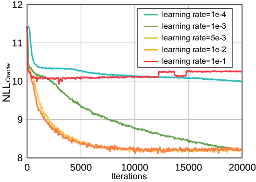
(b) NLL_oracle of CoT

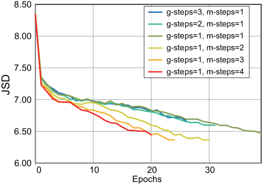
(c) JSD of CoT

Figure 2: Curves of evaluation on JSD, NLL_oracle during iterations of CoT under different training settings. To show the hyperparameter robustness of CoT, we compared it with a typical language GAN i.e. SeqGAN (Yu et al., 2017).

4 Experiments

4.1 Universal Sequence Modeling in Synthetic Turing Test

Following the synthetic data experiment setting in Yu et al. (2017); Zhu et al. (2018), we design a synthetic Turing test, in which the negative log-likelihood NLL_oracle from an oracle LSTM is calculated for evaluating the quality of samples from the generator.

Particularly, to support our claim that our method causes little mode collapse, we calculated NLL_test, which is to sample an extra batch of samples from the oracle, and to calculate the negative log-likelihood measured by the generator.

We show that under this more reasonable setting, our proposed algorithm reaches the state-of-the-art performance with exactly the same network architecture. Note that models like LeakGAN (Guo et al., 2017) contain architecture-level modification, which is orthogonal to our approach, thus will not be included in this part. The results are shown in Table 1. Code for repeatable experiments of this subsection is provided in supplementary materials.

4.1.1 Empirical Analysis of Estimated Gradients

As a part of the synthetic experiment, we demonstrate the empirical effectiveness of the estimated gradient. During the training of CoT model, we record the statistics of the gradient with respect to model parameters estimated by back-propagating $\nabla_{\theta}J^{0.0}_{g}(\theta)$ and $\nabla_{\theta}J^{1.0}_{g}(\theta)$, including the mean and log variance of such gradients.

We are mainly interested in two properties of the estimated gradients, which can be summarized as:

• Bias Obviously, $\nabla_{\theta}J^{1.0}_{g}(\theta)$ is exactly the original gradient which is unbiased towards the minimization of Eq. (13). If the estimated gradient $\nabla_{\theta}J^{0.0}_{g}(\theta)$ is highly biased, the cosine similarity of the average of $\nabla_{\theta}J^{0.0}_{g}(\theta)$ and $\nabla_{\theta}J^{1.0}_{g}(\theta)$ would be close to 0.0, otherwise it would be close to 1.0. To investigate this, we calculate the cosine similarity of expected $\nabla_{\theta}J^{0.0}_{g}(\theta)$ and $\nabla_{\theta}J^{1.0}_{g}(\theta)$.
  

• Variance We calculate the log variance of $\nabla_{\theta}J^{0.0}_{g}(\theta)$ and $\nabla_{\theta}J^{1.0}_{g}(\theta)$ in each dimension, and compute the average log variance of each variance. In the figure, to better illustrate the comparison, we plot the advantage of mean log variance of $\nabla_{\theta}J^{1.0}_{g}(\theta)$ over $\nabla_{\theta}J^{0.0}_{g}(\theta)$. If the variance of the estimated gradient is lower, such a statistic would be steadily positive.

To calculate these statistics, we sample 3,000 sequences from the generator and calculate the average gradient under each settings every 100 iterations during the training of the model. The results are shown in Figure 3. The estimated gradient of our approach shows both properties of low bias and effectively reduced variance.

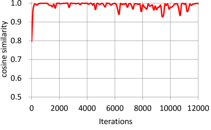
(a) Curves of cosine similarity of averaged $\nabla_{\theta}J^{0.0}_{g}(\theta)$ and $\nabla_{\theta}J^{1.0}_{g}(\theta)$ during training.

(b) Curves of log variance reduction per dimension of $\nabla_{\theta}J^{0.0}_{g}(\theta)$ compared to $\nabla_{\theta}J^{1.0}_{g}(\theta)$

Figure 3: Empirical study on bias and variance comparison.

4.1.2 Discussion

Computational Efficiency Although in terms of time cost per epoch, CoT does not achieve the state-of-the-art, we do observe that CoT is remarkably faster than previous language GANs. Besides, consider the fact that CoT is a sample-based optimization algorithm, which involves time cost in sampling from the generator, this result is acceptable. The result also verifies our claim that CoT has the same order (i.e. the time cost only differs in a constant multiplier or extra lower order term) of computational complexity as MLE.

Hyper-parameter Robustness We perform a hyper-parameter robustness experiment on synthetic data experiment. When compared with the results of similar experiments as in SeqGAN (Yu et al., 2017), our approach shows less sensitivity to hyper-parameter choices, as shown in Figure 2. Note that in all our attempts, the curves of the evaluated JSD of SeqGAN fail to converge.

Self-estimated Training Progress Indicator Like the critic loss, i.e. estimated Earth Mover Distance, in WGANs, we find that the training loss of the mediator (9), namely balanced NLL, can be a real-time training progress indicator as shown in Figure 4. Specifically, in a wide range, balanced NLL is a good estimation of real $JSD(G\|P)$ with a steady translation, namely, $2~{}NLL_{balanced}=2JSD(G\|P)+H(G)+H(P)$.

(a) Curves of $JSD(G\|P)$ during training for MLE, SeqGAN and CoT.

(b) Curves of balanced NLL and real JSD. Both results are from synthetic data experiments.

Figure 4: Training progress curves indicated by different values.

4.2 TextCoT: Zero-prior Long & Diverse Text Generation

As an important sequential data modeling task, zero-prior text generation, especially long and diversified text generation, is a good testbed for evaluating the performance of a generative model.

Following the experiment proposed in LeakGAN (Guo et al., 2017), we choose EMNLP 2017 WMT News Section as our dataset, with maximal sentence length limited to 51. We pay major attention to both quality and diversity. To keep the comparison fair, we present two implementations of CoT, namely CoT-basic and CoT-strong. As for CoT-basic, the generator follows the settings of that in MLE, SeqGAN, RankGAN and MaliGAN. As for CoT-strong, the generator is implemented with the similar architecture in LeakGAN.

For quality evaluation, we evaluated BLEU on a small batch of test data separated from the original dataset. For diversity evaluation, we evaluated the estimated Word Mover Distance (Kusner et al., 2015), which is calculated through training a discriminative model between generated samples and real samples with 1-Lipschitz constraint via gradient penalty as in WGAN-GP (Gulrajani et al., 2017). To keep it fair, for all evaluated models, the architecture and other training settings of the discriminative models are kept the same.

Table 2: N-gram-level quality benchmark: BLEU on test data of EMNLP2017 WMT News.
*: Results under the conservative generation settings as is described in LeakGAN’s paper.

Model	BLEU2	BLEU3	BLEU4	BLEU5
MLE	0.781	0.482	0.225	0.105
SeqGAN	0.731	0.426	0.181	0.096
RankGAN	0.691	0.387	0.178	0.095
MaliGAN	0.755	0.456	0.179	0.088
LeakGAN*	0.835	0.648	0.437	0.271
CoT-basic	0.785	0.489	0.261	0.152
CoT-strong	0.800	0.501	0.273	0.200
CoT-strong*	0.856	0.701	0.510	0.310

Table 3: Diversity benchmark: estimated Word Mover Distance (eWMD) and NLL_test

Model	eWMDtest	eWMDtrain	NLLtest
MLE	1.015 $\sigma$=0.023	0.947 $\sigma$=0.019	2.365
SeqGAN	2.900 $\sigma$=0.025	3.118 $\sigma$=0.018	3.122
RankGAN	4.451 $\sigma$=0.083	4.829 $\sigma$=0.021	3.083
MaliGAN	4.891 $\sigma$=0.061	4.962 $\sigma$=0.020	3.240
LeakGAN	1.803 $\sigma$=0.027	1.767 $\sigma$=0.023	2.327
CoT-basic	0.766 $\sigma$=0.031	0.886 $\sigma$=0.019	2.247
CoT-strong	0.923 $\sigma$=0.018	0.941 $\sigma$=0.016	2.144

The results are shown in Table 2 and Table 3. In terms of generative quality, CoT-basic achieves state-of-the-art performance over all the baselines with the same architecture-level capacity, especially the long-term robustness at n-gram level. CoT-strong using a conservative generation strategy, i.e. setting the inverse temperature parameter $\alpha$ higher than 1, as in (Guo et al., 2017) achieves the best performance over all compared models. In terms of generative diversity, the results show that our model achieves the state-of-the-art performance on all metrics including NLL_test, which is the optimization target of MLE.

Implementation Details of eWMD To calculate eWMD, we adopted a multi-layer convolutional neural network as the feature extractor. We calculate the gradient w.r.t. the one-hot representation $O_{s}$ of the sequence $s$ for gradient penalty. The training loss of the Wasserstein critic $f_{\omega}$ can be formulated as

$$L_{c}(\omega,\lambda)= \mathop{\mathbb{E}}_{s\sim G_{\theta}}\left[f_{\omega}(O_{s})\right]-\mathop{\mathbb{E}}_{s\sim p_{\text{data}}}\left[f_{\omega}(O_{s})\right]$$

$$+\lambda\max(0,\|\nabla f_{\omega}(\hat{O})\|_{2}-1)^{2},$$

where

$$\hat{O}=(1-\mu)O_{s_{p}}+\mu O_{s_{q}}$$

$$\mu\sim\textbf{Uniform}(0,1)$$

$$s_{q}\sim G_{\theta}$$

$$s_{p}\sim p_{\text{data}}.$$

We use Adam (Kingma & Ba, 2014) as the optimizer, with hyper-parameter settings of $\alpha=1e-4$, $\beta_{1}=0.5$, $\beta_{2}=0.9$. For each evaluated generator, we train the critic $f_{\omega}$ for 100,000 iterations, and calculate eWMD($p_{\text{data}},G_{\theta}$) as

$$\mathop{\mathbb{E}}_{s\sim p_{\text{data}}}\left[f_{\omega}(O_{s})\right]-\mathop{\mathbb{E}}_{s\sim G_{\theta}}\left[f_{\omega}(O_{s})\right].$$

The network architecture for $f_{\omega}$ is shown in Table 4.

Table 4: Detailed implementation of eWMD network architecture.

Word Embedding Layer, hidden dim $=128$
Conv1d, window size$=2$, strides$=1$, channels $=64$
Leaky ReLU Nonlinearity ($\alpha=0.2$)
Conv1d, window size$=3$, strides$=2$, channels $=64$
Leaky ReLU Nonlinearity ($\alpha=0.2$)
Conv1d, window size$=3$, strides$=2$, channels $=128$
Leaky ReLU Nonlinearity ($\alpha=0.2$)
Conv1d, window size$=4$, strides$=2$, channels $=128$
Leaky ReLU Nonlinearity ($\alpha=0.2$)
Flatten
Fully Connected, output dimension $=512$
Leaky ReLU Nonlinearity ($\alpha=0.2$)
Fully Connected, output dimension $=1$

5 Future Work & Conclusion

We proposed Cooperative Training, a novel algorithm for training generative models of discrete data. CoT achieves independent success without the necessity of pre-training via maximum likelihood estimation or involving REINFORCE. In our experiments, CoT achieves superior performance on sample quality, diversity, as well as training stability.

As for future work, one direction is to explore whether there is better way to factorize the dropped term of Eq. (14) into some low-variance term plus another high-variance residual term. This would further improve the performance of models trained via CoT. Another interesting direction is to investigate whether there are feasible factorization solutions for the optimization of other distances/divergences, such as Wasserstein Distance, total variance and other task-specific measurements.

6 Acknowledgement

The corresponding authors Sidi Lu and Weinan Zhang thank the support of National Natural Science Foundation of China (61702327, 61772333, 61632017), Shanghai Sailing Program (17YF1428200).

See pages 1,2,3 of cot-appen-icml

References

- Arjovsky & Bottou (2017) Arjovsky, M. and Bottou, L. Towards principled methods for training generative adversarial networks. arXiv preprint arXiv:1701.04862, 2017.
- Arjovsky et al. (2017) Arjovsky, M., Chintala, S., and Bottou, L. Wasserstein gan. arXiv:1701.07875, 2017.
- Bahdanau et al. (2014) Bahdanau, D., Cho, K., and Bengio, Y. Neural machine translation by jointly learning to align and translate. arXiv:1409.0473, 2014.
- Bengio et al. (2015) Bengio, S., Vinyals, O., Jaitly, N., and Shazeer, N. Scheduled sampling for sequence prediction with recurrent neural networks. In NIPS, pp. 1171–1179, 2015.
- Che et al. (2017) Che, T., Li, Y., Zhang, R., Hjelm, R. D., Li, W., Song, Y., and Bengio, Y. Maximum-likelihood augmented discrete generative adversarial networks. arXiv:1702.07983, 2017.
- Goodfellow et al. (2014) Goodfellow, I., Pouget-Abadie, J., Mirza, M., Xu, B., Warde-Farley, D., Ozair, S., Courville, A., and Bengio, Y. Generative adversarial nets. In NIPS, pp. 2672–2680, 2014.
- Gulrajani et al. (2017) Gulrajani, I., Ahmed, F., Arjovsky, M., Dumoulin, V., and Courville, A. C. Improved training of wasserstein gans. In NIPS, pp. 5769–5779, 2017.
- Guo et al. (2017) Guo, J., Lu, S., Cai, H., Zhang, W., Yu, Y., and Wang, J. Long text generation via adversarial training with leaked information. arXiv:1709.08624, 2017.
- Kingma & Ba (2014) Kingma, D. P. and Ba, J. Adam: A method for stochastic optimization. arXiv preprint arXiv:1412.6980, 2014.
- Kusner et al. (2015) Kusner, M., Sun, Y., Kolkin, N., and Weinberger, K. From word embeddings to document distances. In International Conference on Machine Learning, pp. 957–966, 2015.
- Lamb et al. (2016) Lamb, A. M., GOYAL, A. G. A. P., Zhang, Y., Zhang, S., Courville, A. C., and Bengio, Y. Professor forcing: A new algorithm for training recurrent networks. In NIPS, pp. 4601–4609, 2016.
- Lin et al. (2017) Lin, K., Li, D., He, X., Zhang, Z., and Sun, M.-T. Adversarial ranking for language generation. In NIPS, pp. 3155–3165, 2017.
- Lu et al. (2018) Lu, S., Zhu, Y., Zhang, W., Wang, J., and Yu, Y. Neural text generation: Past, present and beyond. arXiv preprint arXiv:1803.07133, 2018.
- Radford et al. (2015) Radford, A., Metz, L., and Chintala, S. Unsupervised representation learning with deep convolutional generative adversarial networks. arXiv preprint arXiv:1511.06434, 2015.
- Ranzato et al. (2015) Ranzato, M., Chopra, S., Auli, M., and Zaremba, W. Sequence level training with recurrent neural networks. arXiv preprint arXiv:1511.06732, 2015.
- Sutton (1984) Sutton, R. S. Temporal credit assignment in reinforcement learning. 1984.
- Ulyanov et al. (2016) Ulyanov, D., Vedaldi, A., and Lempitsky, V. Instance normalization: The missing ingredient for fast stylization. arXiv preprint arXiv:1607.08022, 2016.
- Yu et al. (2017) Yu, L., Zhang, W., Wang, J., and Yu, Y. Seqgan: Sequence generative adversarial nets with policy gradient. In AAAI, pp. 2852–2858, 2017.
- Zhu et al. (2018) Zhu, Y., Lu, S., Zheng, L., Guo, J., Zhang, W., Wang, J., and Yu, Y. Texygen: A benchmarking platform for text generation models. arXiv:1802.01886, 2018.