Abstract

We develop an algorithm for minimizing a function using $n$ batched function value measurements at each of $T$ rounds by using classifiers to identify a function’s sublevel set. We show that sufficiently accurate classifiers can achieve linear convergence rates, and show that the convergence rate is tied to the difficulty of active learning sublevel sets. Further, we show that the bootstrap is a computationally efficient approximation to the necessary classification scheme.

The end result is a computationally efficient derivative-free algorithm requiring no tuning that consistently outperforms other approaches on simulations, standard benchmarks, real-world DNA binding optimization, and airfoil design problems whenever batched function queries are natural.

1 Introduction

Consider the following abstract problem: given access to a function $f\mathrel{\mathop{\mathchar 58\relax}}\mathcal{X}\to\mathbf{R}$, where $\mathcal{X}$ is some space, find $x\in\mathcal{X}$ minimizing $f(x)$. We study an instantiation of this problem that trades sequential access to $f$ for large batches of parallel queries—one can query $f$ for its value over $n$ points at each of $T$ rounds. In this setting, we propose a general algorithm that effectively optimizes $f$ whenever there is a family of classifiers $h\mathrel{\mathop{\mathchar 58\relax}}\mathcal{X}\to[0,1]$ that can predict sublevel sets of $f$ with high enough accuracy.

Our main motivation comes from settings in which $n$ is large—on the order of hundreds to thousands—while possibly small relative to the size of $\mathcal{X}$. These types of problems occur in biological assays [21], physical simulations [27], and reinforcement learning problems [33] where parallel computation or high-throughput measurement systems allow efficient collection of large batches of data. More concretely, consider the optimization of protein binding affinity to DNA sequence targets from biosensor data [11, 21, 38]. In this case, assays measure binding of $n\geq 1000$s of sequences and are inherently parallel due to the fixed costs of setting up an experiment, while the time to measure a collection of sequences makes multiple sequential tests prohibitively time-consuming (so $T$ must be small). In such problems, it is typically difficult to compute the gradients of $f$ (if they even exist); consequently, we focus on derivative-free optimization (DFO, also known as zero-order optimization) techniques.

1.1 Problem statement and approach

The batched derivative free optimization problem consists of a sequence of rounds $t=1,2,\ldots,T$ in which we propose a distribution $p^{(t)}$, draw a sample of $n$ candidates $X_{i}\stackrel{{\scriptstyle{\rm iid}}}{{\sim}}p^{(t)}$, and observe $Y_{i}=f(X_{i})$. The goal is to find at least one example $X_{i}$ for which the gap

$$\min_{i}f(X_{i})-\inf_{x\in\mathcal{X}}f(x)$$

is small.

Our basic idea is conceptually simple: In each round, fit a classifier $h$ predicting whether $Y_{i}\lessgtr\alpha^{(t)}$ for some threshold $\alpha^{(t)}$. Then, upweight points $x$ that $h$ predicts as $f(x)<\alpha^{(t)}$ and downweight the other points $x$ for the proposal distribution $p^{(t)}$ for the next round.

This algorithm is inspired by classical cutting-plane algorithms [30, Sec. 3.2], which remove a constant fraction of the remaining feasible space at each iteration, and is extended into the stochastic setting based on multiplicative weights algorithms [25, 3]. We present the overall algorithm as Algorithm 1.

Algorithm 1 Cutting-planes using classifiers

0:  Objective $f$, Action space $\mathcal{X}$, hypothesis class $\mathcal{H}$.

1:  Set $p^{(0)}(x)=1/|\mathcal{X}|$

2:  Draw $X^{(0)}\sim p^{(0)}$.

3:  Observe $Y^{(0)}=f(X^{(0)})$

4:  for $t\in\{1\ldots T\}$ do

5:     Set $\alpha^{(t)}=\text{median}(\{Y^{(t)}_{i}\}_{i=1}^{n})$

6:     Set $h^{(t)}\in\mathcal{H}$ as the loss minimizer of $L$ over $(X^{(0)},Y^{(0)}>\alpha^{(t)})\ldots(X^{(t-1)},Y^{(t-1)}>\alpha^{(t)})$.

7:     Set $p^{(t)}(x)\propto p^{(t-1)}(x)(1-\eta h^{(t)}(x))$

8:     Draw $X^{(t)}\sim p^{(t)}$

9:     Observe $Y^{(t)}=f(X^{(t)})$.

10:  end for

11:  Set $i^{*}=\arg\min_{i}Y_{i}^{(T)}$

12:  return  $X_{i^{*}}^{(T)}$.

1.2 Related work

When, as is typical in optimization, one has substantial sequential access to $f$, meaning that $T$ can be large, there are a number of major approaches to optimization. Bayesian optimization [34, 7] and kernel-based bandits [9] construct an explicit surrogate function to minimize; often, one assumes it is possible to perfectly model the function $f$. Local search algorithms [12, 26] emulate gradient descent via finite-difference and local function evaluations. Our work differs conceptually in two ways: first, we think of $T$ as being small, while $n$ is large, and second, we represent a function $f$ by approximating its sublevel sets. Existing batched derivative-free optimizers encounter computational difficulties for batch sizes beyond dozens of points [16]. Our sublevel set approach scales to large batches of queries by simply sampling from the current sublevel set approximation.

While other researchers have considered level set estimation in the context of Bayesian optimization [17, 7] and evolutionary algorithms [29], these use the level set to augment a traditional optimization algorithm. We show good sublevel set predictions alone are sufficient to achieve linear convergence. Moreover, given the extraordinary empirical success of modern classification algorithms, e.g. deep networks for image classification [22], it is natural to develop algorithms for derivative-free optimization based on fitting a sequence of classifiers. Yu et al. [40] also propose classification based on optimization, but their approach assumes a classifier constrained to never misclassify near the optimum, making the problem trivial.

1.3 Contributions

We present Algorithm 1 and characterize its convergence rate with appropriate classifiers and show how it relates to measures of difficulty in active learning. We extend this basic approach, which may be computationally challenging, to an approach based on bootstrap resampling that is empirically quite effective and—in certain nice-enough scenarios—has provable guarantees of convergence.

We provide empirical results on a number of different tasks: random (simulated) problems, airfoil (device) design based on physical simulators, and finding strongly-binding proteins based on DNA assays. We show that a black-box approach with random forests is highly effective within a few rounds $T$ of sequential classification; this approach provides advantages in the large batch setting.

The approach to optimization via classification has a number of practical benefits, many of which we verify experimentally. It is possible to incorporate prior knowledge in DFO through domain-specific classifiers, and in more generic optimization problems one can use black-box classifiers such as random forests. Any sufficiently accurate classifier guarantees optimization performance and can leverage the large-batch data collection biological and physical problems essentially necessitate. Finally, one does not even need to evaluate $f$: it is possible to apply this framework with pairwise comparison or ordinal measurements of $f$.

2 Cutting planes via classification

Our starting point is a collection of “basic” results that apply to classification-based schemes and associated convergence results. Throughout this section, we assume we fit classifiers using pairs $(x,z)$, where $z$ is a $0/1$ label of negative (low $f(x)$) or positive (high $f(x)$) class. We begin by demonstrating that two quantities govern the convergence of the optimizer: (1) the frequency with which the classifier misclassifies (and thus downweights) the optimum $x^{*}$ relative to the multiplicative weight $\eta$, and (2) the fraction of the feasible space each iteration removes.

If the classifier $h^{(t)}(x)$ exactly recovers the sublevel set ($h^{(t)}(x)<0$ iff $f(x)<\alpha^{(t)}$), $\alpha^{(t)}$ is at most the population median of $f(X^{(t)})$, and $\mathcal{X}$ is finite, the basic cutting plane bound immediately implies that

$$\log\left[\mathbf{P}_{x\sim p^{(T)}}\left(f(x)=\min_{x^{*}\in\mathcal{X}}f(x^{*})\right)\right]\\ \geq\min\left(T\log\left(\frac{2}{2-\eta}\right)-\log(|\mathcal{X}|),0\right).$$

It is not obvious that such a guarantee continues to hold for inaccurate $h^{(t)}$: it may accidentally misclassify the optimum $x^{*}$, and the thresholds $\alpha^{(t)}$ may not rapidly decrease the function value. To address these issues, we provide a careful analysis in the coming sections: first, we show the convergence guarantees implied by Algorithm 1 as a function of classification errors (Theorem 2.1), after which we propose a classification strategy directly controlling errors (Sec. 2.2), and finally we give a computationally tractable approximation (Sec. 3).

2.1 Cutting plane style bound

We begin with our basic convergence result. Letting $p^{(t)}$ and $h^{(t)}$ be a sequence of distributions and classifiers on $\mathcal{X}$, the convergence rate depends on two quantities: the coverage (number of items cut)

$$\sum_{x\in\mathcal{X}}h^{(t)}(x)p^{(t-1)}(x)$$

and the number of times a hypothesis downweights item $x$ (because $f(x)$ is too large), which we denote $M_{T}(x)\mathrel{\mathop{\mathchar 58\relax}}=\sum_{t=1}^{T}h^{(t)}(x)$. We have the following

Theorem 2.1.

Let $\gamma>0$ and assume that for all $t$,

$$\sum_{x\in\mathcal{X}}h^{(t)}(x)p^{(t-1)}(x)\geq\gamma$$

where $p^{(t)}(x)\propto p^{(t-1)}(x)(1-\eta h^{(t)}(x))$ as in Alg. 1. Let $\eta\in[0,1/2]$ and $p^{(0)}$ be uniform. Then for all $x\in\mathcal{X}$,

$$\log p^{(T)}(x)\geq\frac{\gamma\eta}{\eta+2}T-\eta(\eta+1)M_{T}(x)-\log(2|\mathcal{X}|).$$

The theorem follows from a modification of standard multiplicative weight algorithm guarantees [3]; see supplemental section A.1 for a full proof.

We say that our algorithm converges linearly if $\log p^{(t)}(x)\gtrsim t$. In the context of Theorem 2.1, choice of $\eta$ maximizing $-(\eta^{2}+\eta)M_{T}(x^{*})+\frac{\eta}{\eta+2}\gamma T$ yields such convergence, as picking $\eta$ sufficiently small that

$$T-\frac{(\eta+1)(\eta+2)}{\gamma}M_{T}(x^{*})=\Omega(T)$$

guarantees linear convergence if $2M_{T}(x^{*})<T\gamma$.

A simpler form of the above bound for a fixed $\eta$ shows the linear convergence behavior.

Corollary 1.

Let $x\in\mathcal{X}$, where $q_{T}(x)\mathrel{\mathop{\mathchar 58\relax}}=\frac{M_{T}(x)}{\gamma T}\leq 1/4$. Under the conditions of Theorem 2.1,

$$\log(p^{(T)}(x))\geq\min\left(\frac{1}{5},\frac{1}{3}-\frac{4q_{T}(x)}{3}\right)\frac{\gamma T}{2}-\log(2|\mathcal{X}|)$$

and

$$\frac{1}{4}-\frac{\log(2|\mathcal{X}|)}{2\gamma T}\leq q_{T}(x).$$

The condition $q_{T}(x)\geq\frac{1}{4}-\frac{1}{2\gamma T}\log(2|\mathcal{X}|)$ arises because if $M_{T}(x)$ is small, then eventually we must have $p^{(T)}(x)\geq 1-\gamma$, and any classifier $h$ which fulfils the condition $\sum_{x\in\mathcal{X}}h^{(t)}(x)p^{(t-1)}(x)\geq\gamma$ in Thm. 2.1 must downweight $x$. At this point, we can identify the optimum exactly with $O(1/(1-\gamma))$ additional draws.

The corollary shows that if $M_{T}(x^{*})=0$ and $\gamma=(1-1/e)-1/2<0$, we recover a linear cutting-plane-like convergence rate [cf. 30], which makes constant progress in volume reduction in each iteration.

2.2 Consistent selective strategy for strong control of error

The basic guarantee of Theorem 2.1 requires relatively few mistakes on $x^{*}$, or at least on a point $x$ with $f(x)\approx f(x^{*})$, to achieve good performance in optimization. It is thus important to develop careful classification strategies that are conservative: they do not prematurely cut out values $x$ whose performance is uncertain. With this in mind, we now show how consistent selective classification strategies [15] (related to active learning techniques, and which abstain on “uncertain” examples similar to the Knows-What-It-Knows framework [23, 2]) allow us to achieve linear convergence when the classification problems are realizable using a low-complexity hypothesis class.

The central idea is to only classify an example if all zero-error hypotheses agree on the label, and otherwise abstain. Since any hypothesis achieving zero population error must have zero training set errors, we will only label points in a way consistent with the true labels. El-Yaniv and Wiener [15] define the following consistent selective strategy (CSS).

Definition 2.1 (Consistent selective strategy).

For a hypothesis class $\mathcal{H}$ and training sample $S$, the version space $\mathsf{VS}_{\mathcal{H},S_{m}}\subset\mathcal{H}$ is the set of all hypotheses which perfectly classify $S_{m}$. The consistent selective strategy is the classifier

$$h(x)=\begin{cases}1&\text{ if }\forall g\in\mathsf{VS}_{\mathcal{H},S_{m}},g(x)=1\\ 0&\text{ if }\forall g\in\mathsf{VS}_{\mathcal{H},S_{m}},g(x)=0\\ \text{no decision}&\text{ otherwise.}\end{cases}$$

Applied to our optimizer, this strategy enables safely downweighting examples whenever they are classified as being outside the sublevel set. Optimization performance guarantees then come from demonstrating that at each iteration the selective strategy does not abstain on too many examples.

The rate of abstention for a selective classifier is related to the difficulty of disagreement based active learning, controlled by the disagreement coefficient [18].

Definition 2.2.

The disagreement ball of a hypothesis class $\mathcal{H}$ for distribution $P$ is

$$B_{\mathcal{H},P}(h,r)\mathrel{\mathop{\mathchar 58\relax}}=\{h^{\prime}\in\mathcal{H}\mid P(h(X)\neq h^{\prime}(X))\leq r\}.$$

The disagreement region of a subset $\mathcal{G}\subset\mathcal{H}$ is

$$\mathsf{Dis}(\mathcal{G})\mathrel{\mathop{\mathchar 58\relax}}=\{x\in\mathcal{X}\mid\exists h_{1},h_{2}\in\mathcal{G}\text{ s.t. }h_{1}(x)\neq h_{2}(x)\}.$$

The disagreement coefficient $\Delta_{h}$ of the hypothesis class $\mathcal{H}$ for the distribution $P$ is

$$\Delta_{h}\mathrel{\mathop{\mathchar 58\relax}}=\sup_{r>0}\frac{P(X\in\mathsf{Dis}(B_{\mathcal{H},P}(h,r)))}{r}.$$

The disagreement coefficient directly bounds the abstention rate as a function of generalization error.

Theorem 2.2.

Let $h$ be the CSS classifier in definition 2.1, and let $h^{*}\in\mathcal{H}$ be a classifier achieving zero risk. If $\mathbf{P}(g(X)\neq h^{*}(X))<\epsilon$ for all $g\in\mathsf{VS}_{\mathcal{H},S_{m}}$, then CSS achieves coverage

$$\mathbf{P}(h(X)=\text{no decision})\leq\Delta_{h^{*}}\epsilon$$

This follows from the definition of the disagreement coefficient, and the size of the version space (Supp. section A.1 contains a full proof).

The dependence of our results on the disagreement coefficient implies a reduction from zeroth order optimization to disagreement based active learning [15] and selective classification [39] over sublevel sets.

Implementing the CSS classifier may be somewhat challenging: given a particular point $x$, one must verify that all hypotheses consistent with the data classify it identically. In many cases, this requires training a classifier on the current training sample $S^{(t)}$ at iteration $t$, coupled with $x$ labeled positively, and then retraining the classifier with $x$ labeled negatively [39]. This cost can be prohibitive. (Of course, implementing the multiplicative weights-update algorithm over $x\in\mathcal{X}$ is in general difficult as well, but in a number of application scenarios we know enough about $\mathcal{H}$ to be able to approximate sampling from $p^{(t)}$ in Alg. 1.)

A natural strategy is to use the CSS classifier as part of Algorithm 1, setting all no decision outputs to the zero class, only removing points confidently above the level set $\alpha^{(t)}$. That is, in round $t$ of the algorithm, given samples $S=(X^{(t)},Z^{(t)})$, we define

$$h^{(t)}(x)=\begin{cases}1&\text{ if }\forall g\in\mathsf{VS}_{\mathcal{H},S},g(x)=1\\ 0&\text{ if }\forall g\in\mathsf{VS}_{\mathcal{H},S},g(x)=0\\ 0&\text{ otherwise.}\end{cases}$$

There is some tension between classifying examples correctly and cutting out bad $x\in\mathcal{X}$, which the next theorem shows we can address by choosing large enough sample sizes $n$.

Theorem 2.3.

Let $\mathcal{H}$ be a hypothesis class containing indicator functions for the sublevel sets of $f$, with VC-dimension $V$ and disagreement coefficient $\Delta_{h}$. There exists a numerical constant $C<\infty$ such that for all $\delta\in[0,1]$, $\epsilon\in[0,1]$, and $\gamma\in(\Delta_{h}\epsilon,\frac{1}{2})$, and

$$n\geq\max\Big{\{}C\epsilon^{-1}[V\log(\epsilon^{-1})+\log(\delta^{-1})+\log(2T)],\\ \frac{1}{2(\gamma-0.5)^{2}}(\log(\delta^{-1})+\log(2T))\Big{\}},$$

with probability at least $1-\delta$

$$\log(p^{(T)}(x^{*}))\geq\min\Big{\{}(\gamma-\Delta_{h}\epsilon)\frac{\eta}{\eta+2}T-\log(2|\mathcal{X}|),\\ \log(1-\gamma)\Big{\}}$$

after $T$ rounds of Algorithm 1.

The proof follows from combining the selective classification bound with standard VC dimension arguments to obtain the sample size requirement (Supp. A.1 contains a full proof).

Thus if $\Delta_{h}$ is small, such as $\log(|\mathcal{X}|)$, then choosing $\epsilon=\Delta_{h}^{-1}$ achieves exponential improvements over random sampling. In the worst case, $\Delta_{h}=O(|\mathcal{X}|)$, but small $\Delta_{h}$ are known for many problems, for example for linear classification with continuous $\mathcal{X}$ over densities bounded away from zero, $\Delta_{h}=\text{poly}(\log(\text{Vol}(\mathcal{X})))$, which would result in linear convergence rates (Theorem 7.16, [18]).

Using recent bounds for the disagreement coefficient for linear separators [5], we can show that for linear optimization over a convex domain, the CSS based optimization algorithm above achieves linear convergence with $O(d^{3/2}\log(d^{1/2})-d^{1/2}\log(3T\delta))$ samples with probability at least $1-\delta$ (for lack of space, we present this as Theorem A.2 in the supplement.)

When the classification problem is non-realizable, but the Bayes-optimal hypothesis does not misclassify $x^{*}$, an analogous result holds through the agnostic selective classification framework of Wiener and El-Yaniv [39]. The full result is in supplemental Theorem A.7.

3 Computationally efficient approximations

While selective classification provides sufficient control of error for linear convergence, it is generally computationally intractable. However, a bootstrap resampling algorithm [14] approximates selective classification well enough to provide finite sample guarantees in parametric settings. Our analysis provides intuition for the empirical observation that selective classification via the bootstrap works well in many real-world problems [1].

Formally, consider a parametric family $\{P_{\theta}\}_{\theta\in\Theta}$ of conditional distributions $Z\mid X\in[0,1]$ with compact parameter space $\Theta$. Given $n$ samples $X_{1},\dots,X_{n}$, we observe $Z_{i}|X_{i}\sim P_{\theta^{*}}$ with $\theta^{*}\in\operatorname{int}\Theta$.

Let $\ell_{\theta}(x,z)=-\log(P_{\theta}(z|x))$ be the negative log likelihood of $z$, which majorizes the 0-1 loss of the linear hypothesis class $\ell_{\theta}(x,z)\geq\mathbf{1}_{\left\{(2z-1)x^{\top}\theta<0\right\}}$.

Define the weighted likelihood

$$L_{n}(\theta,u)\equiv\tfrac{1}{n}\sum_{i=1}^{n}(1+u_{i})\ell_{\theta}(X_{i},Z_{i}),$$

and consider the following multiplier bootstrap algorithm [14, 35], parameterized by $B\in\mathbf{N}$ and variance $\sigma^{2}$. $\sigma$ adds additional variation in the estimates to increase parameter coverage.

1. Draw $\{(X_{i},Z_{i})\}_{i=1}^{n}$ from $\mathbf{P}$.

2. Compute $\theta_{n}=\arg\min_{\theta}L_{n}(\theta,0)$.

3. For $b=1$ to $B$,

   1. Draw $u_{b}\stackrel{{\scriptstyle{\rm iid}}}{{\sim}}\mbox{Uni}[-1,1]$.

   2. Compute

      $$\theta^{\circ}_{u_{b}}=\sigma(\arg\min_{\theta}L_{n}(\theta,u_{b})-\theta_{n})+\theta_{n}.$$

4. Define the estimator

   $$h^{\circ}(x)=\begin{cases}1&\text{ if }\forall b\in[B],x^{\top}\theta^{\circ}_{u_{b}}>0\\ 0&\text{ if }\forall b\in[B],x^{\top}\theta^{\circ}_{u_{b}}\leq 0\\ \text{no decision}&\text{ otherwise.}\end{cases}.$$

For linear classifiers with strongly convex losses, this algorithm obtains selective classification guarantees under appropriate regularity conditions as presented in the following theorem.

Theorem 3.1.

Assume $\ell_{\theta}$ is twice differentiable and fulfils $\|\nabla\ell_{\theta}(X,Z)\|\leq R$, and $\left\lVert\nabla^{2}\ell_{\theta}(X,Z)\right\rVert_{op}\leq S$ almost surely. Additionally, assume $L_{n}(\theta,1)$ is $\gamma$-strongly convex and that $\nabla^{2}L_{n}(\theta,1)$ is $M$-Lipschitz with probability one.

For $h^{\circ}$ defined above and $x\in\mathcal{X}$,

$$P(x^{\top}\theta^{*}\leq 0\text{ and }h^{\circ}_{u}(x)=1)<\delta.$$

Further, the abstention rate is bounded by

$$\int_{x\in\mathbf{R}^{d}}\mathbf{1}_{\left\{h^{\circ}_{u}(x)=\emptyset\right\}}p(x)dx\leq\epsilon\Delta_{h}$$

with probability $1-\delta$ whenever

$$B\geq 15\log(3/\delta),$$

$$\sigma=O(d^{1/2}+\log(1/\delta)^{1/2}+n^{-1/2}),$$

$$\epsilon=O\left(\sigma^{2}n^{-1}\log(B/\delta)\right),$$

and

$$n\geq 2\log(2d/\delta)S/\gamma^{2}.$$

Due to length, the proof and full statement with constants appears in the appendix as Theorem A.4, with a sketch provided here: we first show that a given quadratic version space and a multivariate Gaussian sample $\theta^{{\rm quad}}$ obtains the selective classification guarantees (Lemmas A.3,A.4,A.5). We then show that $\theta^{\circ}\approx\theta^{{\rm quad}}$ to order $n^{-1}$ which is sufficient to recover Theorem A.4.

(a) Classification confidences formed by bootstrapping approximate selective classification.

(b) Bootstrapping results in more consistent identification of minima.

Figure 1: Bootstrap consensus provides more conservative classification boundaries which prevents repeatedly misclassifying the minimum, compared to direct loss minimization (panel b, triangle).

The $d\Delta_{h}$ abstention rate in this bound is $d$ times the original selective classification result. This additional factor of $d$ appearing in $\sigma^{2}$ arises from the difference between finding an optimum within a ball and randomly sampling it: random vectors concentrate within $O(1/d)$ of the origin, while the maximum possible value is 1. This gap forces us to scale the variance in the decision function by $\sigma$ (step 3b). We present selective classification approximation bounds analogous to Theorem 2.3 for linear optimization in the Appendix as Theorem A.5.

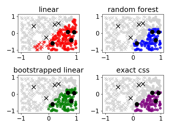
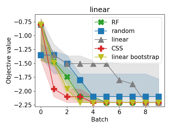
To illustrate our results through simulations, consider a optimizing a two-dimensional linear function in the unit box. Figure 1(a) shows the set of downweighted points (colored points) for various algorithms on classifying a single superlevel set based on eight observations (black points). Observe how linear downweights many points (colored ‘x’), in contrast to exact CSS, which only downweights points guaranteed to be in the superlevel set. Errors of this type combined with Alg. 1 result in optimizers which fail to find the true minimum depending on initialization (Figure 1(b)). The bootstrapped linear classifier behaves similarly to CSS, but is looser due to the non-asymptotic setting. Random forests, another type of bootstrapped classifier is surprisingly good at approximating CSS, despite not making use of the linearity of the decision boundary.

4 Partial order based optimization

One benefit of optimizing via classification is that the algorithm only requires total ordering amongst the elements. Specifically, step 6 of Algorithm 1 only requires threshold comparisons against a percentile selected in step 5. This enables optimization under pairwise comparison feedback. At each round, instead of observing $f(X^{(t)})$, we observe $g(X_{i}^{(t)},X_{j}^{(t)})=1_{f(X_{i}^{(t)})<f(X_{j}^{(t)})}$, which is a natural form of feedback in domains such as human surveys [31] or matched biological experiments [19].

Given the pairwise comparison function $g$, the threshold $f(X^{(t)})<\alpha^{(t)}$ can be replaced with the following stochastic quantile estimator:

$$\hat{f}(X^{(t)}_{i})=\sum_{k=1}^{c}g(X^{(t)}_{I_{k}},X^{(t)}_{i})\leq 0.5,$$ (1)

where $I_{k}\sim\text{Unif}(\{1,2\ldots c\})$ with $cn$ total pairwise comparisons. We show that $c>10$ seems to work well in practice, and more sophisticated preference aggregation algorithms may reduce the number of comparisons even further.

5 Experimental evidence

We evaluate Algorithm 1 as a DFO algorithm across a few real-world experimental design benchmarks, common synthetic toy optimization problems, and benchmarks that allow only pairwise function value comparisons. The small-batch (n = 1-10) nature of hyperparameter optimization problems is outside the scope of our work, even though they are common DFO problems.

For constructing the classifier in Algorithm 1, we apply ensembled decision trees with a consensus decision defined as 75% of trees agreeing on the label (referred to as classify-rf). This particular classifier works in a black-box setting, and is highly effective across all problem domains with no tuning. We also empirically investigate the importance of well-specified hypotheses and consensus ensembling and show improved results for ensembles of linear classifiers and problem specific classifiers, which we call classify-tuned.

In order to demonstrate that no special tuning is necessary, the same constants are used in the optimizer for all experiments, and the classifiers use off-the-shelf implementations from scikit-learn with no tuning.

For sampling points according to the weighted distribution in Algorithm 1, we enumerate for discrete action spaces $\mathcal{X}$, and for continuous $\mathcal{X}$ we perturb samples from the previous rounds using a Gaussian and use importance sampling to approximate the target distribution. Although exact sampling for the continuous case would be time-consuming, the Gaussian perturbation heuristic is fast, and seems to work well enough for the functions tested here.

(a) Binding to the CRX protein

(b) Binding to the VSX1 protein

(c) High-lift airfoil design

Figure 2: Performance on two types of real-world batched zeroth-order optimization tasks. classify-rf consistently outperforms baselines and even randomly sampling twice the batch size. The line shows median function value over runs, shaded area is quartiles.

As a baseline, we compare to the following algorithms

• Random sampling (random)

• Randomly sampling double the batch size (random-2x), which is a strong baseline recently shown to outperform many derivative-free optimizers [24].

• The evolutionary strategy (CMA-ES) for continuous problems, due to its high-performance in black box optimization competitions as well as inherent applicability to the large batch setting [26]

• The Bayesian optimization algorithm provided by GpyOpt[4] (GP) for both continuous and discrete problems, using expected improvement as the acquisition function. We use the ‘random’ evaluator which implements an epsilon-greedy batching strategy, since the large batch sizes (100-1000) makes the use of more sophisticated evaluators completely intractable. The default RBF kernel was used in all experiments presented here. The $\nicefrac{{3}}{{2}}$- and $\nicefrac{{5}}{{2}}$-Matern kernels and string kernels were tried where appropriate, but did not provide any performance improvements.

In terms of runtime, all computations for classify-rf take less than 1 second per iteration compared to 0.1s for CMA-ES and 1.5 minutes for GpyOpt. All experiments were replicated fifteen times to measure variability with respect to initialization.

All new benchmark functions and reference implementations are made available at http://bit.ly/2FgiIxA.

5.1 Designing optimal DNA sequences

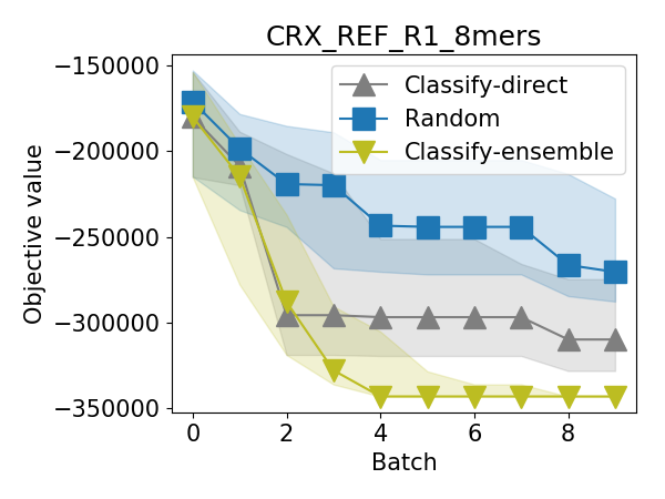
The publicly available protein binding microarray (PBM) dataset consisting of 201 separate assays [6] allows us to accurately benchmark the optimization protein binding over DNA sequences. In each assay, the binding affinity between a particular DNA-binding protein (transcription factor) and all 8-base DNA sequences are measured using a microarray.

This dataset defines 201 separate discrete optimization problems. For each protein, the objective function is the negative binding affinity (as measured by fluorescence), the batch size is 100 (corresponding roughly to the size of a typical 96-well plate), across ten rounds. Each possible action corresponds to measuring the binding affinity of a particular 8-base DNA sequence exactly. The actions are featurized by considering the binary encoding of whether a base exists in a position, resulting in a 32-dimensional space. This emulates the task of finding the DNA binding sequence of a protein using purely low-throughput methods.

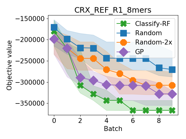
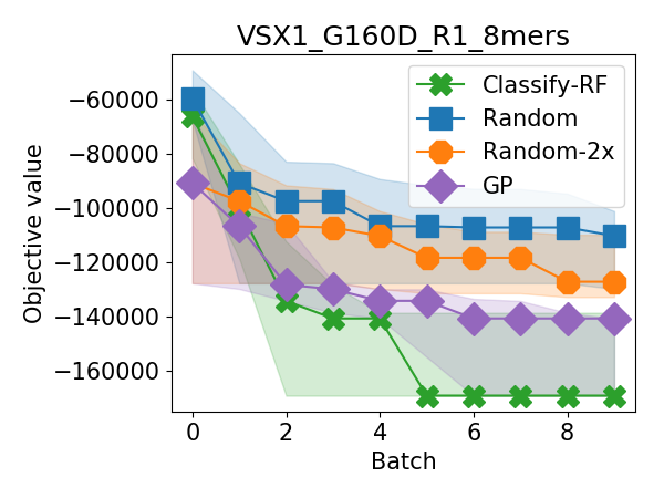
Figure 2(a),2(b) shows the optimization traces of two randomly sampled examples, where the lines indicate median achieved function value over 15 random initializations, and the shading indicates quartiles. classify-rf shows consistent improvements over all discrete action space baselines. For evaluation, we further sample 20 problems and find that the median binding affinity found across replicates is strictly better on 16 out of 20, and tied with the Gaussian process on 2.

In this case, the high performance of random forests is relatively unsurprising, as random forests are known to be high-performance classifiers for DNA sequence recognition tasks [10, 21].

(a) Random linear function

(b) Linear$+$quadratic function

(c) Ensembling classifiers improves optimization performance

Figure 3: Testing the importance of ensembling and well-specified hypothesis class in synthetic data where the hypothesis for Classify-tuned exactly matches level set (panel a), matches level sets with some error (panel b). Ensembling also consistently improves performance, and reduces dependence on initialization (panel c)

5.2 Designing high-lift airfoils

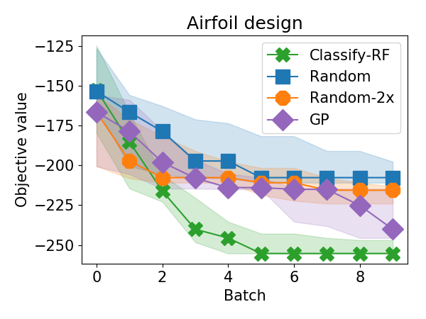
Airfoil design, and other simulator-based objectives are well-suited to the batched, classification based optimization framework, as 30-40 simulations can be run in parallel on modern multicore computers. In the airfoil design case, the simulator is a 2-D aerodynamics simulator for airfoils [13].

The objective function is the negative of lift divided by drag (with a zero whenever the simulator throws an error) and the action space is the set of all common airfoils (NACA-series 4 airfoils). The airfoils are featurized by taking the coordinates around the perimeter of the airfoil as defined in the Selig airfoil format. This results in a highly-correlated two hundred dimensional feature space. The batch size is 30 (corresponding to the number of cores in our machine) and $T=10$ rounds of evaluations are performed.

We find in Figure 2(c) that the classify-rf algorithm converges to the optimal airfoil in only five rounds, and does so consistently, unlike the baselines. The Gaussian process beat the twice-random baseline, since the radial basis kernel is well-suited for this task (as lift is relatively smooth over $\ell_{2}$ distance between airfoils) but did not perform as well as the classify-rf algorithm.

5.3 Gains from designed classifiers and ensembles

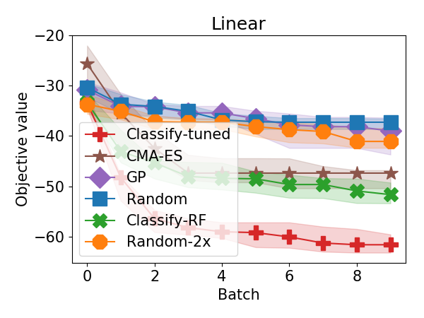
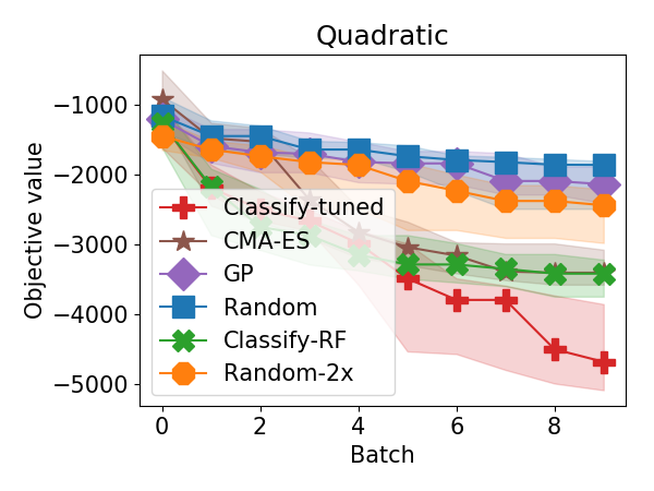
Matching the classifier and objective function generally results in large improvements in optimization performance. We test two continuous optimization problems in $[-1,1]^{300}$, optimizing a random linear function, and optimizing a random sum of a quadratic and linear functions. For this high dimensional task, we use a batch size of 1000. In both cases we compare continuous baselines with classify-rf and classify-tune which uses a linear classifier.

We find that the use of the correct hypothesis class gives dramatic improvements over baseline in the linear case (Figure 3(a)) and continues to give substantial improvements even when a large quadratic term is added, making the hypothesis class misspecified (Figure 3(b)). The classify-rf does not do as well as this custom classifier, but continues to do as well as the best baseline algorithm (CMA-ES).

We also find that using an ensembled classifier is an important for optimization. Figure 3(c) shows an example run on the DNA binding task comparing the consensus of an ensemble of logistic regression classifiers against a single logistic regression classifier. Although both algorithms perform well in early iterations, the single logistic regression algorithm gets ‘stuck’ earlier and finds a suboptimal local minima, due to an accumulation of errors. Ensembling consistently reduces such behavior.

5.4 Low-dimensional synthetic benchmarks

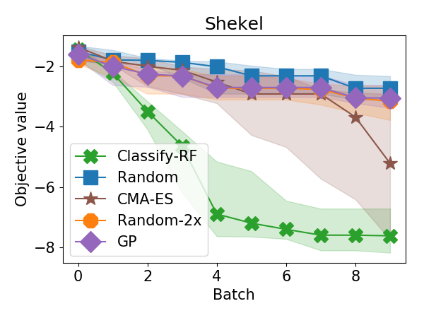
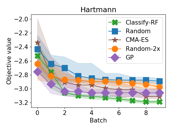
We additionally evaluate on two common synthetic benchmarks (Figure 4(a),4(b)). Although these tasks are not the focus of the work, we show that the classify-rf is surprisingly good as a general black box optimizer when the batch sizes are large.

We consider a batch size of 500 and ten steps due to the moderate dimensionality and multi-modality relative to the number of steps. We find qualitatively similar results to before, with classify-rf outperforming other algorithms and CMA-ES as the best baseline.

(a) Shekel (4d)

(b) Hartmann (6d)

Figure 4: classify-rf outperforms baselines on synthetic benchmark functions with large batches

5.5 Optimizing with pairwise comparisons

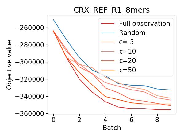
Finally, we demonstrate that we can optimize a function using only pairwise comparisons. In Figure 5 we show the optimization performance when using the ordering estimator from equation 1.

For small numbers of comparisons per element $(c=5)$ we find substantial loss of performance, but once we observe at least 10 pairwise comparisons per proposed action, we are able to reliably optimize as well as the full function value case. This suggests that classification based optimization can handle pairwise feedback with little loss in efficiency.

Figure 5: Optimization with pairwise comparisons between each action and a small set of $(c)$ randomly selected actions. Between 10-20 pairwise comparisons per action gives sufficient information to fully optimize the function.

6 Discussion

Our work demonstrates that the classification-based approach to derivative-free optimization is effective and principled, but leaves open several theoretical and practical questions. In terms of theory, it is not clear whether a modified algorithm can make use of empirical risk minimizers instead of perfect selective classifiers. In practice, we have left the question of tractably sampling from $p^{(t)}$, as well as how to appropriately handle smaller-batch settings of $d>n$.

Appendix A Supplementary materials

A.1 Cutting plane algorithms

See 2.1

Proof.

Since the sampling distribution is derived from multiplicative weights over $\sum_{t=1}^{T}h^{(t)}(x)$, the following regret bound holds with respect to any $p$ (Theorem 2.4, [3]):

$$\gamma T \leq\sum_{t=1}^{T}\sum_{x\in\mathcal{X}}h^{(t)}(x)p^{(t-1)}(x)$$

$$\leq(1+\eta)\sum_{t=1}^{T}\sum_{x\in\mathcal{X}}h^{(t)}(x)p(x)+\frac{\text{KL}(p||p^{(0)})}{\eta}$$

Pick $S=\{i\mathrel{\mathop{\mathchar 58\relax}}\sum_{t}h^{(t)}(x)<\nu T\}$ and $p$ uniform over $S$ to get:

$$\gamma T\leq(1+\eta)\nu T+\frac{\log(|\mathcal{X}|/|S|)}{\eta}$$

From this we get the bound:

$$\log(|S|)\leq\log(|\mathcal{X}|)-\gamma\eta T+\nu\eta T+\nu\eta^{2}T$$

Now we can get the following basic bound on $\log(p^{(T)}(x^{*}))$ by decomposing the normalizer using the set $S$.

$$\log(p^{(T)}(x^{*}))\geq\log(1-\eta)M_{T}(x^{*})$$

$$-\log(|S|+\exp(\log(1-\eta)\nu T)(|\mathcal{X}|-|S|))$$

Note that

$$\exp(\log(1-\eta)\nu T)<\exp(-\eta\nu T)$$

as well as

$$-\eta\nu T=-\gamma\eta T+\nu\eta T+\nu\eta^{2}T$$

whenever $\nu=\gamma/(\eta+2)$. This gives the normalizer bound:

$$\log(|S|+\exp(\log(1-\eta)\nu T)(|\mathcal{X}|-|S|))\\ <\log(2\exp(-\eta\gamma/(\eta+2)T)|\mathcal{X}|)$$

Combining the above:

$$\log(p^{(T)}(x^{*}))$$

$$\geq\log(1-\eta)M_{T}(x^{*})-\log(|S|+\exp(\log(1-\eta)\nu T)|\mathcal{X}|)$$

$$\geq\log(1-\eta)M_{T}(x^{*})-\log(2\exp(-\eta\gamma/(\eta+2)T)|\mathcal{X}|)$$

$$\geq\log(1-\eta)M_{T}(x^{*})+\frac{\eta}{\eta+2}\gamma T-\log(2|\mathcal{X}|)$$

$$\geq-(\eta^{2}+\eta)M_{T}(x^{*})+\frac{\eta}{\eta+2}\gamma T-\log(2|\mathcal{X}|)$$

$$\geq\gamma\frac{\eta}{\eta+2}\left(T-\frac{(\eta+1)(\eta+2)}{\gamma}M_{T}(x^{*})\right)-\log(2|\mathcal{X}|)$$

Where in the second step we use the normalizer bound, and in the third we use the identity $-\log(1-x)\leq x+x^{2}$ for $x\in[0,1/2]$. ∎

See 1

Proof.

First we balance the linear terms in Theorem 2.1 by solving for $\eta$ in

$$\frac{(\eta+1)(\eta+2)}{\gamma}M_{T}(x)=\frac{T}{2}.$$

This gives the multiplicative weight

$$\eta=\min\left(\frac{1}{2},\sqrt{\frac{1}{4}+\frac{1}{2q_{T}(x)}}-\frac{3}{2}\right)>0.$$

The inequality follows from $q_{T}(x)\leq 1/4$ and this reduces the original bound to

$$\log(p^{(T)}(x))\geq\\ \min\left(\frac{1}{5},1+2q_{T}(x)-2\sqrt{2q_{T}(x)+q_{T}(x)^{2}}\right)\frac{\gamma T}{2}\\ -\log(2|\mathcal{X}|).$$

Using the linear lower bound on $1+2q_{T}(x)-2\sqrt{2q_{T}(x)+q_{T}(x)^{2}}$ at $q_{T}(x)=1/4$ gives the first inequality.

The second inequality follows from noting that $\log(p^{(T)}(x))<0$ and solving for $q_{T}(x)$. ∎

See 2.2

Proof.

The inequality follows from two facts. The first fact is that $P(h(X)=\text{no decision})$ is upper bounded by the probability of sampling an $X$ is the disagreement ball of radius $\epsilon$. This follows from the definition of the CSS classifier which outputs no decision if and only if there exists a classifier in $\mathsf{VS}_{\mathcal{H},S_{m}}$ which does not agree with the others, which is the definition of the disagreement region.

The second fact is that if $\sup_{g\in\mathsf{VS}_{\mathcal{H},S_{m}}}P(g(x)\neq h^{*}(x))<\epsilon$, then $\mathsf{VS}_{\mathcal{H},S_{m}}\subseteq B_{\mathcal{H},P}(h^{*},\epsilon)$, by construction of the version space. Applying the definition of the disagreement coefficient completes the proof. ∎

See 2.3

Proof.

The proof has three parts: first, we prove that the median of $n$ samples $Y_{1}\ldots Y_{n}$ is at least the $\gamma$ quantile over $p^{(t)}$.

The probability that the $n$-sample empirical median is less than the $\gamma$ quantile over $p^{(t)}$ is equivalent to having $X\sim\text{Binom}(\gamma,n)$ and $\mathbf{P}(X>n/2)$. Applying Hoeffding’s inequality,

$$\mathbf{P}(X>n/2)\leq\exp(-2(\gamma-0.5)^{2}n).$$

Next, we show that the CSS prediction abstains on at most $\Delta_{h}\epsilon$ fraction of the distribution. VC dimension bounds [20] imply that we can achieve $\epsilon$ error uniformly over hypothesis class $\mathcal{H}$ with VC dimension $V$ in

$$n=C\epsilon^{-1}[V\log(\epsilon^{-1})+\log(\delta^{\prime-1})]$$

samples with probability at least $1-\delta$ for some constant $C$. We can then apply the CSS classifier bound to get that the abstention rate is $\Delta_{h}\epsilon$. This implies:

$$\sum_{x\in\mathcal{X}}h^{(t)}(x)p^{(t-1)}(x)\geq\gamma-\Delta_{h}\epsilon$$ (2)

Finally, whenever $p^{(t)}(x^{*})<\frac{1}{1-\gamma}$,

$$h(x^{*})=1_{f(x^{*})\leq\alpha^{(t)}}=0,$$

and thus $M_{t}(x^{*})=0$.

The $\log(p^{(T)})$ inequality follows by applying Theorem 2.1 with Equation 5 noting that either $M_{T}(x^{*})=0$ or $p^{(T)}(x^{*})>\frac{1}{1-\gamma}$.

Union bounding the above two probabilities, and ensuring each part has failure probability $\delta/2$,

$$n=\max\big{(}C\epsilon^{-1}[V\log(\epsilon^{-1})+\log(\delta^{-1})+\log(2T)],\\ \frac{1}{2(\gamma-0.5)^{2}}(\log(\delta^{-1})+\log(2T))\big{)}$$

implies $\delta$ failure probability. ∎

A.2 Convergence rates for optimizing linear functions

.

The first lemma generalizes Theorem 2.1 to the continuous case.

Lemma A.1.

Consider a compact $\mathcal{X}\subset\mathbb{R}^{d}$ and $\gamma>0$, and let $(h^{(t)}\mathrel{\mathop{\mathchar 58\relax}}\mathcal{X}\to[0,1],p^{(t-1)})_{t\in\mathbf{N}}$ be a sequence such that for every $t\in\mathbf{N}$,

$$\int_{x}h^{(t)}(x)p^{(t-1)}(x)dx\geq\gamma,$$

$$p^{(t)}(x)\propto p^{(t-1)}(x)(1-\eta h^{(t)}(x))$$

for some $\eta\in[0,1/2]$, and $p^{(0)}$ the uniform distribution over $\mathcal{X}$. Further, let $M_{T}(x)=\sum_{t=1}^{T}h^{(t)}(x)$ the number of times $h^{(t)}$ downweights item $x$. Then the following bound on density at the any item $x^{*}$ holds on the last step:

$$\log(p^{(T)}(x))\geq\gamma\frac{\eta}{\eta+2}\left(T-\frac{(\eta+1)(\eta+2)}{\gamma}M_{T}(x)\right)\\ -\log(\text{vol}(\mathcal{X})/2)\\$$

Proof.

Since the sampling distribution is derived from multiplicative weights over $\sum_{t=1}^{T}h^{(t)}(x)$, the following regret bound holds with respect to any $p$ (Theorem 2.4, [3]):

$$\gamma T \leq\sum_{t=1}^{T}\int_{x\in\mathcal{X}}h^{(t)}(x)p^{(t-1)}(x)dx$$

$$\leq(1+\eta)\sum_{t=1}^{T}\int_{x\in\mathcal{X}}h^{(t)}(x)p(x)dx+\frac{\text{KL}(p||p^{(0)})}{\eta}$$

Pick $S=\{x\in\mathcal{X}\mathrel{\mathop{\mathchar 58\relax}}\sum_{t}h^{(t)}(x)<\nu T\}$ and $p$ uniform over $S$ to get:

$$\gamma T\leq(1+\eta)\nu T+\frac{\log(\text{vol}(\mathcal{X})/\text{vol}(S))}{\eta}$$

From this we get the bound:

$$\log(\text{vol}(S))\leq\log(\text{vol}(\mathcal{X}))-\gamma\eta T+\nu\eta T+\nu\eta^{2}T$$

Now we can get the following basic bound on $\log(p^{(T)}(x^{*}))$ by decomposing the normalizer using $S$.

$$\log(p^{(T)}(x^{*}))\geq\log(1-\eta)M_{T}(x^{*})$$

$$-\log(\text{vol}(S)+\exp(\log(1-\eta)\nu T)(\text{vol}(\mathcal{X})-\text{vol}(S)))$$

The rest of the proof is identical to that of Theorem 1 and we obtain:

$$\log(p^{(T)}(x^{*}))$$

$$\geq\gamma\frac{\eta}{\eta+2}\left(T-\frac{(\eta+1)(\eta+2)}{\gamma}M_{T}(x^{*})\right)-\log(2\text{vol}(\mathcal{X})).$$

∎

We now show that given a well-behaved starting distribution, the distribution induced by the multiplicative weights algorithm is close to a uniform distribution over the sublevel set.

Lemma A.2.

Define $h^{*(t)}(x)=1_{f(x)\leq\alpha^{(t)}}$ and $q^{(t)}(x)=\frac{1-h^{*(t)}(x)}{\int_{x\in\mathcal{X}}1-h^{*(t)}(x)dx}$.

Define $p^{(t)}$ and $h^{(t)}$ such that

$$p^{(t-1)}(x)\propto 1\quad\forall x\mathrel{\mathop{\mathchar 58\relax}}h^{*(t)}(x)=1,$$

$$\int_{x\in\mathcal{X}}h^{(t)}(x)p^{(t-1)}(x)dx=\gamma,$$

$$p^{(t)}(x)\propto p^{(t-1)}(x)(1-\eta h^{(t)}(x)).$$

and further, $\int_{x\in\mathcal{X}}1_{h^{*(t)}(x)=0}1_{h^{(t)}(x)=1}dx=0$ and $\int_{x\in\mathcal{X}}1_{h^{*(t)}(x)=1}1_{h^{(t)}(x)=0}p^{(t-1)}(x)dx\leq\nu$ then

$$\frac{1-\eta(\gamma-\nu)}{1-\gamma-\nu}p^{(t)}(x)\geq q^{(t)}(x)$$

for all $x\in\mathcal{X}$.

Proof.

We verify the inequality on $S^{*}=\{x\mathrel{\mathop{\mathchar 58\relax}}h^{*(t)}(x)=0\}$, since $q^{(t)}(x)$ is zero outside $S^{*}$.

For any $x\in S^{*}$, $q^{(t)}(x)=1/\text{vol}(S^{*})$ and $p^{(t-1)}(x)\geq(1-\gamma-\nu)/\text{vol}(S^{*})$.

This implies for $x\in S^{*}$,

$$p^{(t)}(x)\geq\frac{(1-\gamma-\nu)/\text{vol}(S^{*})}{\int_{x\in\mathcal{X}}p^{(t-1)}(x)(1-\eta h^{(t)}(x))}.$$

We now upper bound the normalizer:

$$\int_{x\in\mathcal{X}}p^{(t-1)}(x)(1-\eta h^{(t)}(x)) \leq 1-\eta\int_{x\in\mathcal{X}}p^{(t-1)}(x)h^{(t)}(x)$$

$$\leq 1-\eta(\gamma-\nu).$$

This gives the bound that for all $x\in S^{*}$,

$$\frac{1-\eta(\gamma-\nu)}{1-\gamma-\nu}p^{(t)(x)}\geq q^{(t)}(x).$$

∎

The next theorem gives the disagreement coefficient for linear classification in a log-concave density.

Theorem A.1 (Theorem 14, [5]).

Let $\mathcal{D}$ be a log-concave density in $\mathbb{R}^{d}$ and $\mathcal{H}$ the set of linear classifier in $\mathbb{R}^{d}$, then the region of disagreement over error in Definition 2.2 is:

$$\frac{\mathbf{P}_{X\sim\mathcal{D}}(X\in\mathsf{Dis}(B(h,r)))}{r}=O(d^{1/2}\log(1/r)).$$

Proof.

The statement here is identical to [5] with the exception of the identity covariance constraint on $\mathcal{D}$. We omit this due to the equivalence of isotropic and non-isotropic cases as noted in Appendix C, Theorem 6. ∎

Finally, we combine the above results to obtain convergence rates on the linear optimization with linear classifier case.

Theorem A.2.

Let $f(x)=w^{\top}x$ for some $w$, and $\mathcal{X}$ a convex subset of $\mathbb{R}^{D}$. Define $p^{(0)}$ as uniform on $\mathcal{X}$.

Define the classification label $Z_{i}=1_{Y_{i}>\text{median}(Y)}$, on which we train a CSS classifier over the linear hypothesis class $\mathcal{H}$ which we define as

$$h^{(t)}(x)=\begin{cases}1&\text{ if }\forall g\in\mathsf{VS}_{\mathcal{H},(X,Z)},g(x)=1\\ 0&\text{ if }\forall g\in\mathsf{VS}_{\mathcal{H},(X,Z)},g(x)=0\\ 0&\text{ otherwise }.\end{cases}$$

Define the sampling distributions for each step

$$p^{(t)}(x)\propto p^{(t-1)}(x)(1-h^{(t)}(x)/2)$$

Then for any small $\nu$, a batch size of

$$n^{(t)}=O\left(\frac{d^{3/2}}{\nu}\log(\nu^{-1}d^{1/2})-\frac{d^{1/2}}{\nu}\log(3T\delta)\right),$$

is sufficient to establish the following bound on sampling items below any $\alpha$ level set $S_{\alpha}=\{x\in\mathcal{X}\mathrel{\mathop{\mathchar 58\relax}}f(x)<\alpha\}$ on the last step:

$$\log\left(\int_{x\in S_{\alpha}}p^{(T)}(x)\right)\geq\\ \min\bigg{(}\left(\frac{1}{4}-\nu\right)\frac{1}{5}T-\log(2\text{vol}(\mathcal{X}))+\log(\text{vol}(S_{\alpha})),\\ -\log(4)\bigg{)}$$

with probability $1-\delta$.

Proof.

We will begin by using induction to show that at each round $t$ the abstention rate is at most $\nu$. In the base case of $t=0$, $p^{(0)}(x)$ is log-concave and we can apply Theorem A.1 and 2.2, which implies $\nu=C_{1}d^{1/2}\log(1/\epsilon)\epsilon$. VC dimension bounds imply there exists some $n=C_{2}\epsilon^{-1}(d\log(1/\epsilon)+\log(1/\delta_{1}))$ such that any consistent hypothesis incurs at most $\epsilon$ population error.

Inverting and solving for $n$ shows that for some $C$,

$$n^{0}\geq C\nu^{-1}d^{1/2}[d\log(\nu^{-1}d^{1/2})+\log(\delta_{1}^{-1})]$$

is sufficient to guarantee $\nu$-abstention.

For each round $t>0$ assume we maintained $\nu$-abstention in all prior rounds. We then fulfil the condition of Lemma A.2. To verify each condition: $p^{(t-1)}(x)$ is constant on sublevel sets below $\alpha^{(t)}$ since the selective classifier to never makes false positives, by construction. $\eta=1/2$, $\gamma^{(t)}$ is the population quantile of $p^{(t-1)}$ corresponding to $\text{median}(Y^{(t-1)})$ and $\nu$ is the abstention rate at round $t-1$.

Lemma A.2 states that if a sample drawn $x\sim p^{(t)}$ has $f(x)<\text{median}(Y^{(t-1)})=\alpha^{(t-1)}$, then this sample follows the uniform distribution over the sublevel set $S_{\alpha^{(t-1)}}$ and that the probability of this event occuring is at least $\frac{1-\gamma^{(t)}-\nu}{1-(\gamma^{(t)}-\nu)/2}$.

Thus, if we sample $n^{\prime}$ samples from $p^{(t)}$, then with probability at least $1-\delta_{2}$, $n$ of these draws will be from a uniform distribution in the $\alpha^{(t)}$ sublevel set, where $\delta_{2}$ follows:

$$\delta_{2}=\mathbf{P}\left(\sum_{i=1}^{n^{\prime}}1_{X^{(t)}_{i}\in S_{\alpha^{(t-1)}}}\leq n\right)\\ \leq\exp\left(-2\left(\frac{1-\gamma^{(t)}-\nu}{1-(\gamma^{(t)}-\nu)/2}-n/n^{\prime}\right)^{2}n^{\prime}\right)$$

Solving for $n^{\prime}$, with the shorthand $\tau=\frac{1-\gamma^{(t)}-\nu}{1-(\gamma^{(t)}-\nu)/2}$ and $\delta_{2}<1$,

$$n^{\prime} \geq\frac{\sqrt{\log(\delta_{2})(\log(\delta_{2})-8\tau n)}+4\tau n-\log(\delta_{2})}{4\tau^{2}}$$

$$\geq\frac{1}{\tau}n-\frac{\log(\delta_{2})}{2\tau^{2}}$$

Since the $\alpha^{(t)}$ sublevel set is convex, we can apply Theorem A.1 to these $n$ samples contained in the sublevel set to show that for all $t>0$,

$$n\geq C\nu^{-1}d^{1/2}[d\log(\nu^{-1}d^{1/2})+\log(\delta_{1}^{-1})]$$

samples is sufficient to ensure $\nu$-abstention when we train a selective classifier on $n$ points. Learning a selective classifier over all $n^{\prime}$ points can only decrease the abstention region, and therefore $n^{t}$ is sufficient to guarantee $\nu$ abstention.

Combining with the bound on $n^{\prime}$, with probability $1-\delta_{2}-\delta_{1}$,

$$n^{(t)}\geq\frac{1}{\tau}C\nu^{-1}d^{1/2}[d\log(\nu^{-1}d^{1/2})+\log(\delta_{1}^{-1})]-\frac{\log(\delta_{2})}{4\tau^{2}}$$

Next, we bound $\gamma$ from above and below using the same argument as Theorem 2.3. At any round $t$ defining $\gamma^{(t)}=\int_{x\in\mathcal{X}}p^{(t-1)}(x)1_{x<\text{median}(Y^{(t-1)})}$ by Hoeffding’s inequality the probability $\gamma^{(t)}$ is within $[1/4,3/4]$ is:

$$\mathbf{P}(1/4\leq\gamma^{(t)}\leq 3/4)\geq 1-2\exp(-n^{(t)}/8).$$

Thus, we can ensure $\gamma^{(t)}\in[1/4,3/4]$ with probability at least $1-\delta_{3}$ in round $t$ if we have

$$n^{(t)}\geq-8\log(\delta_{3}/2).$$

Simplifying the bounds, we can ensure $\nu$ abstention across all $T$ rounds with probability at least $1-\delta$ given $\tau=\frac{1/4-\nu}{7/8+\nu/2}$.

$$n^{(t)}\geq C\frac{7/8+\nu/2}{1/4\nu-\nu^{2}}d^{1/2}[d\log(\nu^{-1}d^{1/2})-\log(3T\delta)]\\ -\frac{\log(3T\delta)(7/8+\nu/2)^{2}}{4(1/4-\nu)^{2}}\\ +8\log(3T\delta^{-1})$$

Collecting first order terms for $\nu$ small we have

$$n^{(t)}=O\left(\frac{d^{3/2}}{\nu}\log(\nu^{-1}d^{1/2})-\frac{d^{1/2}}{\nu}\log(3T\delta)\right)$$

Finally, we can apply Lemma A.1 to get a lower bound for all points $x\mathrel{\mathop{\mathchar 58\relax}}f(x)<\alpha^{(T)}$.

$$\log(p^{(T)}(x))\geq\left(\frac{1}{4}-\nu\right)\frac{1}{5}T-\log(2\text{vol}(\mathcal{X})).$$

The complete bound with respect to the $\alpha$ sublevel set follows after checking two cases. If $\alpha^{(T)}\geq\alpha$, then the entire set $\{x\mathrel{\mathop{\mathchar 58\relax}}f(x)<\alpha\}$ follows the lower bound, and we integrate to obtain the first part of the bound. If $\alpha^{(T)}<\alpha$ then by construction of $\alpha^{(T)}$, at least $1-\gamma$ of the distribution must lie below $\alpha^{(T)}$ and thus we draw an element with function value less than $\alpha^{(T)}<\alpha$ with probability at least $\log(1-\gamma)$. ∎

A.3 Approximating selective sampling with Gaussians

In this section, we show that sampling from a particular Gaussian approximates selective classification for linear classification with strongly convex losses.

First, we show that the maximum over sampled Gaussian parameter vectors is close to the infimum over an hyperellipse.

Lemma A.3.

Consider $\theta^{{\rm quad}}_{1}\ldots\theta^{{\rm quad}}_{B}\sim N(\hat{\theta},\Sigma)$ then for any $x$ and $Q_{\tau}=\{\theta\mathrel{\mathop{\mathchar 58\relax}}(\theta-\hat{\theta})^{\top}\Sigma^{-1}(\theta-\hat{\theta})\leq 2\tau\}$,

$$P\left(\min_{i}x^{\top}\theta^{{\rm quad}}_{i}-\inf_{\theta\in Q_{\tau}}x^{\top}\theta>\sqrt{x^{\top}\Sigma x}\epsilon\right)\\ \leq(1-\Phi(\epsilon-\sqrt{2\tau}))^{B}.$$

Where $\Phi$ is the cumulative distribution function of the standard Gaussian.

Proof.

We can whiten the space with $\Sigma^{-1/2}$ to get the following equivalent statement:

Define $\overline{\theta^{{\rm quad}}}_{i}=\Sigma^{-1/2}\theta^{{\rm quad}}_{i}$, then $\overline{\theta^{{\rm quad}}}_{1}\ldots\overline{\theta^{{\rm quad}}}_{B}\sim N(0,I)$ and let $\overline{x}=\Sigma^{1/2}x$,

$$\mathbf{P}\left(\min_{i}x^{\top}\theta^{{\rm quad}}_{i}-\inf_{\theta\in Q_{\tau}}x^{\top}\theta>\sqrt{x^{\top}\Sigma x}\epsilon\right)$$

$$\quad=P\left(\min_{i}\overline{x}^{\top}\overline{\theta^{{\rm quad}}}_{i}-\inf_{\theta\mathrel{\mathop{\mathchar 58\relax}}\left\lVert\theta\right\rVert_{2}^{2}<2\tau}\overline{x}^{\top}\theta>\left\lVert\overline{x}\right\rVert_{2}\epsilon\right)$$

$$\quad=P\left(\min_{i}\frac{\overline{x}^{\top}}{\left\lVert\overline{x}\right\rVert_{2}}\overline{\theta^{{\rm quad}}}_{i}>\epsilon-\sqrt{2\tau}\right)$$

$$\quad=P\left(\frac{\overline{x}^{\top}}{\left\lVert\overline{x}\right\rVert_{2}}\overline{\theta^{{\rm quad}}}_{0}>\epsilon-\sqrt{2\tau}\right)^{B}$$

$$\quad=(1-\Phi(\epsilon-\sqrt{2\tau}))^{B}$$

∎

For $\epsilon=0$ and $\tau=1$, if $B\geq\log(\delta)/\log(0.95)$ then the minimum of the $B$ samples is smaller than the infimum over the $\Sigma^{-1}$ ellipse with probability at least $1-\delta$.

Next, we show that the samples from $N(\hat{\theta},\Sigma)$ in $d$-dimensions are contained in a ball a constant factor larger than $d\Sigma^{-1}$ with high probability.

Lemma A.4.

Let $\theta^{{\rm quad}}_{1}\ldots\theta^{{\rm quad}}_{B}\sim N(\hat{\theta},\Sigma)$, then:

$$P\left(\max_{i}(\theta^{{\rm quad}}_{i}-\hat{\theta})^{\top}\Sigma^{-1}(\theta^{{\rm quad}}_{i}-\hat{\theta})^{\top}\geq cd\right)\\ \leq B\left(c\exp\left(1-c\right)\right)^{d/2}$$

for $c>1$.

Proof.

Since $(\theta^{{\rm quad}}_{i}-\hat{\theta})^{\top}\Sigma^{-1}(\theta^{{\rm quad}}_{i}-\hat{\theta})^{\top}$ is whitened, we can define the probability in terms of chi-squared variables $\xi_{1}\ldots\xi_{B}\sim\chi^{2}(d)$.

$$P\left(\max_{i}(\theta^{{\rm quad}}_{i}-\hat{\theta})^{\top}\Sigma^{-1}(\theta^{{\rm quad}}_{i}-\hat{\theta})^{\top}\geq cd\right)$$

$$\quad=P\left(\max_{i}\xi_{i}\geq cd\right)$$

$$\quad=1-P\left(\xi_{0}<cd\right)^{B}$$

$$\quad\leq 1-\left(1-\left(c\exp\left(1-c\right)\right)^{d/2}\right)^{B}$$

$$\quad\leq B\left(c\exp\left(1-c\right)\right)^{d/2}$$

Which implies

$$\max_{i}(\theta^{{\rm quad}}_{i}-\hat{\theta})^{\top}\Sigma^{-1}(\theta^{{\rm quad}}_{i}-\hat{\theta})\\ <4\log(2B/d)+2d-4\log(\delta/2)$$

with probability $1-\delta$.

∎

Thus for $c=1+O\left(\frac{2}{d}\left(\log(B)-\log(\delta)\right)\right)$, we can ensure that all $B$ samples are contained in the $cd\Sigma^{-1}$ ball with probability at least $1-\delta$.

Combining the two results, we can show that for a quadratic version space, we can perform selective classification by sampling from a Gaussian.

Theorem A.3.

Define the selective classifier with respect to a set $Q$ (a subset of the parameter space $\Theta$) as:

$$h_{Q}(x)=\begin{cases}1&\text{ if }\forall\theta\in Q,\theta^{\top}x>0\\ 0&\text{ if }\forall\theta\in Q,\theta^{\top}x\leq 0\\ \emptyset&\text{ otherwise }\end{cases}.$$

Let $Q_{\tau}=\{\theta\mathrel{\mathop{\mathchar 58\relax}}(\theta-\hat{\theta})^{\top}\Sigma^{-1}(\theta-\hat{\theta})<2\tau\}$ and $\theta^{{\rm quad}}_{1}\ldots\theta^{{\rm quad}}_{B}\sim N(\hat{\theta},\Sigma)$.

Then the sampled selective classifier:

$$h^{\text{quad}}(x)=\begin{cases}1&\text{ if }\forall\theta^{{\rm quad}}_{i},x^{\top}\theta^{{\rm quad}}_{i}>0\\ 0&\text{ if }\forall\theta^{{\rm quad}}_{i},x^{\top}\theta^{{\rm quad}}_{i}\leq 0\\ \emptyset&\text{ otherwise }\end{cases}.$$

Has the following properties.

For any $x\in\mathcal{X}$

$$P(h_{Q_{\tau}}(x)=0\text{ and }h^{\text{quad}}(x)=1)\leq(1-\Phi(-\sqrt{2\tau}))^{B}$$

and for any $c>1$,

$$P\left(\sum_{x}1_{h_{Q_{cd}}(x)}=\emptyset<\sum_{x}1_{h^{\text{quad}}(x)=\emptyset}\right)\\ \leq B\left(c\exp\left(1-c\right)\right)^{d/2}$$

Proof.

The first statement follows directly from Lemma A.3, since having $h_{Q_{\tau}}(x)=0$ and $h^{\text{quad}}(x)=1$ is a subset of the event that is upper bounded in Lemma A.3.

The second statement follows from Lemma A.4. Under the conditions of the theorem,

$$P\bigg{(}\max_{i}(\theta^{{\rm quad}}_{i}-\hat{\theta})^{\top}\Sigma^{-1}(\theta^{{\rm quad}}_{i}-\hat{\theta})^{\top})\geq cd\bigg{)}\\ \leq B\left(c\exp\left(1-c\right)\right)^{d/2}.$$

If $\max_{i}(\theta^{{\rm quad}}_{i}-\hat{\theta})^{\top}\Sigma^{-1}(\theta^{{\rm quad}}_{i}-\hat{\theta})^{\top}\geq cd$, then for all $i$, $\theta^{{\rm quad}}_{i}\in Q_{cd}.$

By construction, if $h^{\text{quad}}(x)=\emptyset$ then, $h_{Q_{cd}(x)}=\emptyset$ since at least one pair of $\theta^{{\rm quad}}_{i}$ must disagree, and this pair must also be in $Q_{cd}(x)$. ∎

Now we show that a quadratic version space contains the Bayes optimal parameter, and is contained in a version space with low error. We first state a result on the strong convexity of the empirical loss, which follows immediately from Theorem 5.1.1 of [36].

Lemma A.5.

Let $\{P_{\theta}\}_{\theta\in\Theta}$ be a parametric family over a compact parameter space $\Theta$. Define $Z\mid X\sim P_{\theta^{*}}$ for some $\theta^{*}\in\operatorname{int}\Theta$.

Let $\ell_{\theta}(x,z)=-\log(P(z\mid x))$ be the negative log likelihood of $z$, and

$$L_{n}(\theta)=\tfrac{1}{n}\sum_{i=1}^{n}\ell_{\theta}(X_{i},Z_{i}).$$

If

$$\lambda_{\text{min}}\left(\mathbf{E}\left[\nabla^{2}\ell_{\theta}(X,Z)\right]\right)\geq\gamma,~{}\text{and}$$

$$\lambda_{\text{max}}\left(\nabla^{2}\ell_{\theta}(X,Z)\right)\leq L~{}\text{w.p. 1},$$

then

$$\lambda_{\text{min}}\left(\nabla^{2}L_{n}(\theta)\right)\geq\left(1-\sqrt{\frac{2L\log(\nicefrac{{d}}{{\delta}})}{n\gamma}}\right)\gamma$$

with probability $1-\delta$.

We now define the three possible version spaces that we can consider - the version space of the low error hypotheses $VS$, version space of low-loss models $\ell$, and the quadratic approximation $Q$.

Definition A.1.

Define the maximum likelihood estimator $\theta_{n}=\arg\min_{\theta\in\Theta}L_{n}(\theta)$

The quadratic version space with radius $\tau$ around $L_{n}$ is

$$Q_{\tau}=\bigg{\{}\theta\mathrel{\mathop{\mathchar 58\relax}}\nabla L_{n}(\theta_{n})^{\top}(\theta-\theta_{n})+\tfrac{1}{2}(\theta-\theta_{n})^{\top}\\ \nabla^{2}L_{n}(\theta_{n})(\theta-\theta_{n})\leq\tau\bigg{\}}.$$

The version space of loss-loss parameters $\theta$ with radius $\tau$ is

$$\mathcal{L}_{\tau}=\bigg{\{}\theta\mathrel{\mathop{\mathchar 58\relax}}L_{n}(\theta)-L_{n}(\theta_{n})\leq\tau\bigg{\}}.$$

The version space of a set of hypotheses $h$ with error less than $\tau$ is

$$VS_{\tau}=\bigg{\{}\theta\mathrel{\mathop{\mathchar 58\relax}}P\left(h_{\theta}(X)\not=Z\right)-P\left(h_{\theta_{n}}(X)\not=Z\right)\leq\tau\bigg{\}}.$$

Lemma A.6.

In the same settings as lemma A.5, assume $\ell_{\theta}(x,z)$ majorizes the zero one loss for some hypothesis class $\mathcal{H}=\{h_{\theta}\mathrel{\mathop{\mathchar 58\relax}}\theta\in\Theta\}$ as $\ell_{\theta}(x,z)\geq\mathbf{1}_{\left\{h_{\theta}(x)=z\right\}}$, $\|\nabla\ell_{\theta}(X,Z)\|\leq R$ almost surely, and $\nabla^{2}L_{n}(\theta)$ is $M$-Lipschitz.

Then, for the version spaces given in definition A.1,

$$VS_{\tau+2\zeta}\supseteq\mathcal{L}_{\tau+2\zeta}\supseteq Q_{\tau+\zeta}\supseteq\mathcal{L}_{\tau},$$ (3)

where $\zeta=M\left(\tfrac{\tau}{2\gamma}\right)^{\nicefrac{{3}}{{2}}}$. Furthermore, if

$$\tau=\frac{36\nu_{0}^{2}}{C_{f}^{2}}\frac{2.7d+\log(\nicefrac{{1}}{{\delta}})}{n},$$

then $\theta^{*}\in Q_{\tau}$ with probability $1-\delta$ where constants $C_{f}$ and $\nu_{0}$ defined in [35] as

$$C_{f}\leq\sup_{\theta}\frac{D_{\text{kl}}\left(\theta,\theta^{*}\right)}{\|I^{-\nicefrac{{1}}{{2}}}(\theta-\theta^{*})\|},~{}\text{and}$$

$$\nu_{0}^{2}\geq R\lambda_{\text{max}}(I_{\theta^{*}}).$$

Proof.

The norm $\|\theta-\theta_{n}\|$ bounds the remainder term of the 2nd order Taylor expansion of $L_{n}$ from above,

$$L_{n}(\theta) -L_{n}(\theta_{n})\leq\nabla L_{n}(\theta_{n})^{\top}(\theta-\theta_{n})$$

$$+\tfrac{1}{2}(\theta-\theta_{n})^{\top}\nabla^{2}L_{n}(\theta_{n})(\theta-\theta_{n})$$

$$+\|R(\theta,\theta_{n})\|_{\text{op}}\|\theta-\theta_{n}\|^{2},$$

and below,

$$L_{n}(\theta) -L_{n}(\theta_{n})\geq\nabla L_{n}(\theta_{n})^{\top}(\theta-\theta_{n})$$

$$+\tfrac{1}{2}(\theta-\theta_{n})^{\top}\nabla^{2}L_{n}(\theta_{n})(\theta-\theta_{n})$$

$$-\|R(\theta,\theta_{n})\|_{\text{op}}\|\theta-\theta_{n}\|^{2},$$

with $\|R(\theta,\theta_{n})\|_{\text{op}}\leq M\|\theta-\theta_{n}\|$.

First, we prove $\mathcal{L}_{\tau}\subseteq Q_{\tau+\zeta}$.

Let $\theta\in\mathcal{L}_{\tau}$. Strong convexity of $L_{n}$ at $\theta_{n}$ implies

$$\|\theta-\theta_{n}\|^{2}\leq\frac{2}{\gamma}(L_{n}(\theta)-L_{n}(\theta_{n}))\leq\frac{2}{\gamma}\tau.$$

Using this in the Taylor expansion above implies

$$\nabla L_{n}(\theta_{n})^{\top}(\theta-\theta_{n})+\tfrac{1}{2}(\theta-\theta_{n})^{\top}\nabla^{2}L_{n}(\theta_{n})(\theta-\theta_{n})$$

$$\begin{aligned} &\leq L_{n}(\theta)-L_{n}(\theta_{n})+\|R(\theta,\theta_{n})\|_{\text{op}}\|\theta-\theta_{n}\|^{2}\\ &\leq\tau+M\left(\frac{2\tau}{\gamma}\right)^{\tfrac{3}{2}}=\tau+\zeta.\end{aligned}$$

The argument to show $Q_{\tau}\subseteq\mathcal{L}_{\tau+\zeta}$ is nearly identical.

Strong convexity of $L_{n}$ implies strong convexity of its quadratic expansion with the same parameter. Let $\theta\in Q_{\tau}$. The above Taylor approximation shows

$$L_{n}(\theta)-L_{n}(\theta_{n})\leq$$

$$\begin{aligned} &\nabla L_{n}(\theta_{n})^{\top}(\theta-\theta_{n})+\tfrac{1}{2}(\theta-\theta_{n})^{\top}\nabla^{2}L_{n}(\theta_{n})(\theta-\theta_{n})\\ &+\|R(\theta,\theta_{n})\|_{\text{op}}\|\theta-\theta_{n}\|^{2}\\ &\leq\tau+M\left(\frac{2\tau}{\gamma}\right)^{\tfrac{3}{2}}=\tau+\zeta.\end{aligned}$$

That $\ell(\delta,z)$ majorizes the 0-1 loss almost immediately implies $\mathcal{L}_{\tau}\subseteq VS_{\tau}$. Indeed, $L_{n}(\theta)\leq\tau$ implies $\frac{1}{n}\sum\mathbf{1}_{\left\{h_{\theta}(X_{i})\not=Z_{i}\right\}}\leq\tau$, and so $h_{\theta}$ is in $VS_{\tau}$.

That $Q_{\tau}$ contains $\theta^{*}$ with probability $1-\delta$ follows from Theorem 5.2 of [35] with the stated constants. ∎

A.4 Approximating selective sampling with the bootstrap

We begin by showing the minimizer of the quadratic approximation is close to the $\theta^{{\rm quad}}_{u}$ we defined.

Define

$$L_{n}(\theta,u)\mathrel{\mathop{\mathchar 58\relax}}=\frac{1}{n}\sum_{i=1}^{n}L_{i}(\theta)+\frac{1}{n}\sum_{i=1}^{n}u_{i}L_{i}(\theta),$$

which is convex for all $u\geq-\mathbf{1}$. The standard negative log-likelihood is then $L_{n}(\theta,\mathbf{0})$, and for simplicity in notation (and to reflect the dependence on $u$) we let $\theta_{n}=\mathop{\rm argmin}_{\theta}L_{n}(\theta,\mathbf{0})$ and $\theta_{u}=\mathop{\rm argmin}_{\theta}L_{n}(\theta,u)$. Recall that we assume that $\theta\mapsto\nabla^{2}L_{i}(\theta)$ is $M$-Lipschitz (in operator norm) and $L_{n}(\theta,\mathbf{0})$ is $\gamma$-strongly convex.

We collect a few identification and complexity results.

Lemma A.7 (Rakhlin and Sridharan [32]).

Let $u_{i}$ be independent, mean-zero, $\sigma^{2}$-sub-Gaussian random variables. Then for any sequence of vectors $v_{i}$ with $\left\lVert v_{i}\right\rVert\leq R$ for each $i$,

$$\mathbf{P}\left(\left\lVert\sum_{i=1}^{n}u_{i}v_{i}\right\rVert\geq cR\sigma\sqrt{n}(1+t)\right)\leq\exp(-t^{2}),$$

where $c<\infty$ is a numerical (universal) constant.

We then have the following guarantee.

Lemma A.8.

Let $\left\lVert\nabla L_{i}(\theta)\right\rVert\leq R$ for all $i$ and $u_{i}$ be independent mean-zero $\sigma^{2}$-sub-Gaussian random variables. Then there exist numerical constants $C_{1},C_{2},C_{3}<\infty$ such that for all $t\in\mathbf{R}$ and $n\geq\frac{d}{\gamma^{2}}C_{2}(C_{3}-\log(\delta))$, we have

$$\left\lVert\theta_{u}-\theta_{n}\right\rVert\leq C_{1}\cdot\frac{R\sigma}{\sqrt{n}}$$

with probability at least $1-\delta$.

Proof.

The proof is a more or less standard exercise in localization and concentration [8]. We begin by noting that $|u_{i}|$ is $O(1)\sigma^{2}$-sub-Gaussian, so that $\frac{1}{n}\sum_{i=1}^{n}|u_{i}|\leq\mathbf{E}[|u_{i}|]+t$ with probability at least $1-\exp(-cnt^{2}/\sigma^{2})$, where $c>0$ is a numerical constant, so we assume that $\sum_{i=1}^{n}|u_{i}|\leq 2\sigma$, which occurs with probability at least $1-e^{-cn}$. Non-asymptotic lower bounds on the eigenvalues of random matrices [28, Thm. 1.3] imply that for any $t\geq 0$,

$$\nabla^{2}L_{n}(\theta_{n};u)\succeq\left(\gamma-\sqrt{\frac{d}{n}}\cdot t\right)I_{d}$$ (4)

with probability at least $1-\exp(-ct^{2}+C\log\log t)$ for constants $c>0$, $C<\infty$. Then using the $M$-Lipschitz continuity of $\nabla^{2}L$, we obtain

$$\left\lVert\nabla^{2}L_{n}(\theta;u)-\nabla^{2}L_{n}(\theta_{n};u)\right\rVert_{\rm op} \leq\frac{M}{n}\sum_{i=1}^{n}|u_{i}|\left\lVert\theta-\theta_{n}\right\rVert$$

$$\leq 2M\sigma\left\lVert\theta-\theta_{n}\right\rVert.$$

With this identification, for all $\theta$ satisfying $\left\lVert\theta-\theta_{n}\right\rVert\leq\frac{\epsilon}{2M\sigma}$, we have

$$L_{n}(\theta,u) \geq L_{n}(\theta_{n},u)+\langle\nabla L_{n}(\theta_{n},u),\theta-\theta_{n}\rangle$$

$$\qquad~{}+\frac{\gamma-\epsilon-t\sqrt{d/n}}{2}\left\lVert\theta-\theta_{n}\right\rVert^{2}$$

with probability at least $1-\exp(-ct^{2}+C\log\log t)$. Now, using Lem A.7, we obtain that $\left\lVert\nabla L_{n}(\theta_{n};u)\right\rVert\leq\frac{cR\sigma}{\sqrt{n}}(1+t)$ with probability at least $1-e^{-t^{2}}$, so that we have

$$L_{n}(\theta,u) \geq L_{n}(\theta_{n},u)-\frac{CR\sigma}{\sqrt{n}}(1+t)\left\lVert\theta_{n}-\theta\right\rVert$$

$$\qquad~{}~{}+\frac{\gamma-\epsilon-t\sqrt{d/n}}{2}\left\lVert\theta_{n}-\theta\right\rVert^{2}$$

with probability at least $1-2e^{-ct^{2}+C\log\log t}$, where $0<c,C<\infty$ are numerical constants.

Now fix $\epsilon$. Solving the above quadratic in $\left\lVert\theta_{n}-\theta\right\rVert$, we have that

$$\left\lVert\theta-\theta_{n}\right\rVert>\frac{2CR\sigma}{\sqrt{n}(\gamma-\epsilon)-t\sqrt{d}}$$

implies that $L_{n}(\theta,u)>L_{n}(\theta_{n},u)$. If we assume for simplicity $\epsilon=\gamma/2$, then we have that

$$\frac{\gamma}{2}\geq\left\lVert\theta-\theta_{n}\right\rVert>\frac{4CR\sigma}{\sqrt{n}\gamma-2t\sqrt{d}}$$

implies that $L_{n}(\theta,u)>L_{n}(\theta_{n},u)$, or (by convexity) that any minimizer $\theta_{u}$ of $L_{n}(\theta,u)$ must satisfy $\left\lVert\theta_{u}-\theta_{n}\right\rVert\leq\frac{4CR\sigma}{\sqrt{n}\gamma-2t\sqrt{d}}$.

The resulting bound states that there exists numerical constants $c>0$, $C<\infty$ such that for all $t\in\mathbf{R}$, we have

$$\left\lVert\theta_{u}-\theta_{n}\right\rVert\leq C\frac{R\sigma}{\sqrt{n}}\cdot\frac{1}{\gamma-2t\sqrt{d/n}}$$

with probability at least $1-Ce^{-ct^{2}+\log\log(t)}$.

Upper bounding $\log(\log(t))\leq\log(t)$ and solving for $t$, for any $t\geq C_{2}\sqrt{C_{3}-\log(\delta)}$ there exists $C_{2},C_{3}<\infty$ such that $1-Ce^{-ct^{2}+\log(\log(t))}>1-\delta$.

Finally, if $n\geq\frac{d}{\gamma}^{2}C_{2}^{2}(C_{3}-\log(\delta))$, then we have an upper bound,

$$\left\lVert\theta_{u}-\theta_{n}\right\rVert\leq 2C\frac{R\sigma}{\sqrt{n}}$$

with probability at least $1-\delta$.

∎

Define the minimizer for a quadratic approximation to the multiplier bootstrap loss as

$$\theta^{{\rm quad}}_{u}\mathrel{\mathop{\mathchar 58\relax}}=\theta_{n}-\nabla^{2}L_{n}(\theta_{n})^{-1}\frac{1}{n}\sum_{i=1}^{n}u_{i}\nabla L_{i}(\theta_{n}).$$

We now show that for subgaussian $u$, $\theta^{{\rm quad}}_{u}\approx\theta_{u}$.

Lemma A.9.

Let $\left\lVert\nabla L_{i}(\theta)\right\rVert\leq R$, $\left\lVert\nabla^{2}L_{i}(\theta_{n})\right\rVert_{\rm op}\leq S$ for all $i$, and $u_{i}$ be independent mean-zero $\sigma^{2}$-sub-Gaussian random variables. Then there exist numerical constants $C,C_{1},C_{2},C_{3}<\infty$ such that for all $\delta>0$ and $n\geq\frac{d}{\gamma^{2}}C_{2}(C_{3}-\log(\delta/4))$,

$$\left\lVert\theta_{u}-\theta^{{\rm quad}}_{u}\right\rVert\leq C\frac{R^{2}\sigma^{2}}{n}\left(2M+\frac{S\sqrt{\log(4d/\delta)}}{R}\right)$$

with probability at least $1-\delta$.

Proof.

By definition, we have

$$\theta^{{\rm quad}}_{u}\mathrel{\mathop{\mathchar 58\relax}}=\theta_{n}-\nabla^{2}L_{n}(\theta_{n})^{-1}\frac{1}{n}\sum_{i=1}^{n}u_{i}\nabla L_{i}(\theta_{n}).$$

Now, consider $\theta_{u}$. By Taylor’s theorem and the $M$-Lipschitz continuity of $\nabla^{2}L_{i}$, we have that for matrices $E_{i}\mathrel{\mathop{\mathchar 58\relax}}\mathbf{R}^{d}\to\mathbf{R}^{d\times d}$ with $\left\lVert E_{i}(\theta)\right\rVert_{\rm op}\leq M\left\lVert\theta-\theta_{n}\right\rVert$ that for all $\theta$ near $\theta_{n}$, we have

$$\sum_{i=1}^{n}(1+u_{i})\nabla L_{i}(\theta)$$

$$=n\nabla^{2}L_{n}(\theta_{n})(\theta-\theta_{n})+\sum_{i=1}^{n}u_{i}\nabla L_{i}(\theta_{n})$$

$$~{}+\sum_{i=1}^{n}E_{i}(\theta)(\theta-\theta_{n})+\sum_{i=1}^{n}u_{i}\left[\nabla^{2}L_{i}(\theta_{n})+E_{i}(\theta)\right](\theta_{u}-\theta_{n}).$$

That is, defining the random matrix

$$E\mathrel{\mathop{\mathchar 58\relax}}=\frac{1}{n}\sum_{i=1}^{n}\left[(1+u_{i})E_{i}(\theta_{u})+u_{i}\nabla^{2}L_{i}(\theta_{n})\right]$$

and noting that $\mathbf{0}=\frac{1}{n}\sum_{i=1}^{n}(1+u_{i})\nabla L_{i}(\theta_{u})$, we have

$$-\frac{1}{n}\sum_{i=1}^{n}u_{i}\nabla L_{i}(\theta_{n})=\left(\nabla^{2}L_{n}(\theta_{n})+E\right)(\theta_{u}-\theta_{n}).$$

Using standard matrix concentration inequalities [36] yields that

$$\mathbf{P}\left(\left\lVert\sum_{i=1}^{n}u_{i}\nabla^{2}L_{i}(\theta_{n})\right\rVert_{\rm op}\geq t\right)\leq 2d\exp\left(-\frac{ct^{2}n}{\sigma^{2}S^{2}}\right)$$

for a numerical constant $c>0$. Using that $\left\lVert E_{i}(\theta)\right\rVert_{\rm op}\leq M\left\lVert\theta-\theta_{n}\right\rVert$, we obtain that with probability at least $1-2d\exp(-\frac{ct^{2}n}{\sigma^{2}S^{2}})$, thus we have $\left\lVert E\right\rVert_{\rm op}\leq 2M\left\lVert\theta_{u}-\theta\right\rVert+\frac{S\sigma\sqrt{\log(2d/\delta)}}{\sqrt{2}}$ with probability at least $1-\delta$. Using Lem A.8, we have that for all $n\geq\frac{d}{\gamma^{2}}C_{2}(C_{3}-\log(\delta/4))$,

$$\theta_{u}=\theta_{n}-\left(\nabla^{2}L_{n}(\theta_{n})+E\right)^{-1}\frac{1}{n}\sum_{i=1}^{n}u_{i}\nabla L_{i}(\theta_{n})$$

with probability at least $1-\delta$, where $\left\lVert E\right\rVert_{\rm op}\leq 2CM\frac{R\sigma}{\sqrt{n}}+\frac{S\sigma\sqrt{\log(4d/\delta)}}{\sqrt{2n}}.$

Now we use the fact that if $\left\lVert EA^{-1}\right\rVert_{\rm op}<1$ for symmetric matrices $A,E$, then $(A+E)^{-1}=A^{-1}\sum_{i=0}^{\infty}(-1)^{i}(EA^{-1})^{i}$. Using our bounds on $2M\epsilon_{n}+t<\frac{1}{2\gamma}$, we have

$$(\nabla^{2}L_{n}(\theta_{n})+E)^{-1}=\nabla^{2}L_{n}(\theta_{n})^{-1}+\tilde{E},$$

where the matrix $\tilde{E}$ satisfies $\|{\tilde{E}}\|_{\rm op}\leq 2\left\lVert E\right\rVert_{\rm op}$. Applying Lem A.7 gives the result. ∎

We now define the constant terms of the bootstrap error into a function $\psi$ to simplify notation for the remaining sections.

Definition A.2 (Bootstrap error constants).

Under the conditions of Lemma A.9, define

$$\psi(n,d,\delta)=C\frac{R^{2}}{n}\left(2M+\frac{S\sqrt{\log(4d/\delta)}}{R}\right).$$

Now note that if $u_{i}\sim U(-1,1)$ then $\mathbf{E}[\theta^{{\rm quad}}_{u}]=\theta_{n}$ and $\textbf{Cov}[\theta^{{\rm quad}}_{u}]=\nabla^{2}L_{n}(\theta_{n},0)^{-1}\sum_{i=1}^{n}\nabla L_{i}(\theta)\nabla L_{i}(\theta)^{\top}\nabla^{2}L_{n}(\theta_{n},0)^{-1}\sigma^{2}/n$, which is close to the distribution used in the Gaussian sampling section before.

We now show that for $\theta^{\circ}_{u}\mathrel{\mathop{\mathchar 58\relax}}=\rho(\theta_{u}-\theta_{n})+\theta_{n}$, $\left\lVert\theta^{\circ}_{u}-\theta^{{\rm quad}}_{u}\right\rVert_{2}$ is small enough to make the quadratic approximation hold for the bootstrap samples.

Lemma A.10.

Under the conditions of Lemma A.8 and A.9, define $\theta^{\circ}_{u_{1}}\ldots\theta^{\circ}_{u_{B}}$ where $\theta^{\circ}_{u_{i}}\mathrel{\mathop{\mathchar 58\relax}}=\sigma(\theta_{u_{i}}-\theta_{n})+\theta_{n}$ and $u_{ij}\sim U(-1,1)$.

For any $x$ and $Q_{\tau/n}=\{\theta\mathrel{\mathop{\mathchar 58\relax}}(\theta-\theta_{n})^{\top}\nabla^{2}L_{n}(\theta,0)(\theta-\theta_{n})\leq\tau/n\}$.

$$\min_{i}x^{\top}\theta_{u_{i}}^{\circ}-\inf_{\theta\in Q_{\tau/n}}x^{\top}\theta\leq 0$$

with probability at least $1-\delta$ whenever

$$B \geq\log(\delta/3)/\log(1-\Phi(1)/2)$$

$$n \geq\max\left(\frac{8R^{2}}{3S}\log(3d/\delta),4C^{2}S^{4}R^{2}\gamma^{-2}/\Phi(1)^{-2}\right)$$

$$\sigma \geq\sqrt{2\tau}\frac{\left(1+\frac{\sqrt{8}\gamma^{-7/2}S^{2}R}{\sqrt{3}(1+S)}\sqrt{\log(2d/\delta)}\right)}{\left(1-\psi(n,d,\delta)S\gamma^{-1/2}\right)}$$

where $\psi$ is defined in Definition A.2.

Proof.

The proof proceeds in two parts: in the first, we bound the mismatch between the covariance matrix of $\theta^{{\rm quad}}_{u}$ and $\nabla^{2}L_{n}(\theta_{n})^{-1}$. In the second part, we bound the gap between $\theta^{\circ}$ and $\theta^{{\rm quad}}$.

Define the covariance matrix $\Sigma=\nabla^{2}L_{n}(\theta)^{-1}\sum_{i=1}^{n}\nabla L_{i}(\theta)\nabla L_{i}(\theta)^{\top}\nabla^{2}L_{n}(\theta)^{-1}/n$, the whitened samples $\overline{x}=\Sigma^{1/2}x$, and whitened parameters $\overline{\theta}^{\circ}_{u}=\Sigma^{-1/2}(\theta^{\circ}_{u}-\theta_{n})$.

By whitening and applying the operator norm bound we obtain the upper bound

$$\min_{i}x^{\top}\theta_{u_{i}}^{\circ}-\inf_{\theta\in Q_{\tau/n}}x^{\top}\theta$$

$$=\min_{i}\overline{x}^{\top}\overline{\theta}^{\circ}_{u_{i}}-\inf_{\left\lVert\theta\right\rVert_{2}^{2}\in 2\tau}\overline{x}^{\top}\Sigma^{-1/2}\nabla^{2}L_{n}(\theta)^{-1/2}\theta/\sqrt{n}$$

$$\leq\left\lVert\overline{x}\right\rVert_{2}\bigg{(}\min_{i}\frac{\overline{x}^{\top}}{\left\lVert\overline{x}\right\rVert_{2}}\overline{\theta}^{\circ}_{u_{i}}$$

$$\qquad+\sqrt{2\tau}\left\lVert I-\Sigma^{-1/2}\nabla^{2}L_{n}(\theta)^{-1/2}/\sqrt{n}\right\rVert_{op}\bigg{)}.$$

The second term is the error from the quadratic approximation, and we can bound this via the Ando-Hemmen inequality (Proposition 3.2, [37]) which states $\left\lVert A^{1/2}-B^{1/2}\right\rVert\leq\frac{1}{\left\lVert A^{-1/2}\right\rVert_{op}^{-1}+\left\lVert B^{-1/2}\right\rVert_{op}^{-1}}\left\lVert A-B\right\rVert_{op}$, which gives

$$\left\lVert I-\Sigma^{-1/2}\nabla^{2}L_{n}(\theta)^{-1/2}/\sqrt{n}\right\rVert_{op}$$

$$\leq\frac{n^{-1/2}\left\lVert\Sigma^{-1/2}\sqrt{n}\right\rVert_{op}\left\lVert\Sigma n-\nabla^{2}L_{n}(\theta)^{-1}\right\rVert_{op}}{\left\lVert\Sigma^{-1/2}\sqrt{n}\right\rVert_{op}^{-1}+\left\lVert\nabla^{2}L_{n}(\theta)^{1/2}\right\rVert^{-1}}$$

$$\leq\frac{\sqrt{n}\gamma^{-7/2}}{S^{-3/2}+S^{-1/2}}\left\lVert\sum_{i=1}^{n}\nabla L_{i}(\theta)\nabla L_{i}(\theta)^{\top}-\nabla^{2}L_{n}(\theta)\right\rVert_{op}.$$

Finally, applying the Matrix Bernstein inequality (Thm 6.1.1, [36]),

$$\left\lVert I-\Sigma^{-1/2}\nabla^{2}L_{n}(\theta)^{-1/2}\right\rVert_{op}\\ \leq\frac{\sqrt{8}\gamma^{-7/2}S^{2}R}{\sqrt{3}(1+S)}\sqrt{\log(d/\delta)}$$

with probability at least $1-\delta$, when $n\geq\frac{8R^{2}}{3S}\log(d/\delta)$.

For the other parts of the bound let $\overline{\theta^{{\rm quad}}}_{u_{i}}=\Sigma^{1/2}(\theta^{{\rm quad}}_{u_{i}}-\theta_{n})$ which is a $d$-dimensional unit Gaussian with variance $\sigma^{2}$. By Lemma A.8,

$$\min_{i}x^{\top}\theta_{u_{i}}^{\circ}-\inf_{\theta\in Q_{\tau/n}}x^{\top}\theta$$

$$\leq\left\lVert\overline{x}\right\rVert_{2}\bigg{(}\min_{i}\frac{\overline{x}^{\top}}{\left\lVert\overline{x}\right\rVert_{2}}\overline{\theta^{{\rm quad}}}_{u_{i}}$$

$$\qquad+\psi(n,d,\delta/3)S\gamma^{-1/2}\sigma$$

$$\qquad+\sqrt{2\tau}\left(1+\frac{\sqrt{8}\gamma^{-7/2}S^{2}R}{\sqrt{3}(1+S)}\sqrt{\log(3d/\delta)}\right)$$

with probability $1-2\delta/3$. Define

$$\sigma=\sqrt{2\tau}\frac{\left(1+\frac{\sqrt{8}\gamma^{-7/2}S^{2}R}{\sqrt{3}(1+S)}\sqrt{\log(2d/\delta)}\right)}{1-\psi(n,d,t)S\gamma^{-1/2}}.$$

Since $\overline{x}^{\top}\overline{\theta^{{\rm quad}}}$ is a bounded i.i.d sum of $n$ gradient terms, by the Berry-Esseen theorem there exists a universal constant $C$ such that

$$P\left(\min_{i}x^{\top}\theta_{u_{i}}^{\circ}-\inf_{\theta\in Q_{\tau/n}}x^{\top}\theta\leq 0\right)\\ \leq\left(1-\Phi(\tau)+\frac{CS^{2}R}{\gamma\sqrt{n}}\right)^{B}.$$

If $B\geq\log(\delta/3)/\log(1-\Phi(1)/2)$ and $n\geq 4C^{2}S^{4}R^{2}\gamma^{-2}/\Phi(1)^{-2}$, we have that:

$$\min_{i}x^{\top}\theta_{u_{i}}^{\circ}-\inf_{\theta\in Q_{\tau/n}}x^{\top}\theta\leq 0$$

with probability at least $1-\delta$.

∎

Thus to satisfy the same bounds as the bootstrap, we must expand the ellipse under consideration by a small multiplicative factor.

We first define the bootstrap based selective classifier.

Definition A.3.

Let $\{P_{\theta}\}_{\theta\in\Theta}$ be a parametric family over a compact parameter space $\Theta$. Define $Z\mid X\sim P_{\theta^{*}}$ for some $\theta^{*}\in\operatorname{int}\Theta$.

Let $\ell_{\theta}(x,z)=-\log(P(z\mid x))$ be the negative log likelihood of $z$, and assume that $\|\nabla\ell_{\theta}(X,Z)\|\leq R$ and $\left\lVert\nabla^{2}\ell(X,Z)\right\rVert_{op}\leq S$ almost surely and this majorizes the 0-1 loss of a linear classifier, $\ell_{\theta}(x,z)\geq\mathbf{1}_{\left\{(2z-1)x^{\top}\theta<0\right\}}$.

Define the weighted sample negative log likelihood

$$L_{n}(\theta,u)\mathrel{\mathop{\mathchar 58\relax}}=\tfrac{1}{n}\sum_{i=1}^{n}(1+u_{i})\ell_{\theta}(X_{i},Z_{i}),$$

and we assume $L_{n}(\theta,0)$ to be $\gamma$-strongly convex and $\nabla^{2}L_{n}(\theta,0)$ to be $M$-Lipschitz.

Given a scaling constant $\sigma>0$, define the $B$ bootstrapped estimators $\theta^{\circ}_{u_{i}}=\sigma(\theta_{u}-\theta_{n})+\theta_{n}$ with $u_{i1}\ldots u_{in}\sim U(-1,1)$.

The bootstrap selective classifier is defined as

$$h^{\circ}_{u}(x)\mathrel{\mathop{\mathchar 58\relax}}=\begin{cases}1&\text{ if }\forall i,x^{\top}\theta^{\circ}_{u_{i}}>0\\ 0&\text{ if }\forall i,x^{\top}\theta^{\circ}_{u_{i}}\leq 0\\ \emptyset&\text{ otherwise }\end{cases}.$$

Combining the above results in the following bootstrap based selective classification bound.

Theorem A.4.

The bootstrap selective classifier in definition A.3 fulfils

$$\int_{x\in\mathbf{R}^{d}}\mathbf{1}_{\left\{h^{\circ}_{u}(x)=0\text{ and }x^{\top}\theta^{*}\geq 0\right\}}p(x)dx\leq\epsilon,$$

$$\int_{x\in\mathbf{R}^{d}}\mathbf{1}_{\left\{h^{\circ}_{u}(x)=\emptyset\right\}}p(x)dx\leq\epsilon\Delta_{h},$$

and for any $x$,

$$P(x^{\top}\theta^{*}\leq 0\text{ and }h^{\circ}_{u}(x)=1)<\delta$$

with probability at least $1-\delta$ whenever

$$B\geq\log(\delta/3)/\log(\Phi(1)),$$

$$\sigma=\sqrt{\frac{72\nu_{0}^{2}}{C_{f}^{2}}(2.7d+\log\left(\nicefrac{{3}}{{\delta}}\right))}\frac{\bigg{(}1+\frac{\sqrt{8}\gamma^{-7/2}S^{2}R}{\sqrt{3}(1+S)}\sqrt{\log(2d/\delta)}\bigg{)}}{1-\psi(n,d,\delta/2)S\gamma^{-1/2}}\\ =O(d^{1/2}+\log(1/\delta)^{1/2}),$$

$$\epsilon\geq\bigg{(}2\frac{\sigma^{2}\nu}{n}+M\left(\frac{\sigma^{2}\nu}{2n\gamma}\right)^{3/2}\bigg{)}=O(\sigma^{2}/n),$$

$$\nu=C\frac{R^{2}S}{n}$$

and

$$n\geq 2\log(2d/\delta)S/\gamma^{2}.$$

The constants $C_{f}$ and $\nu_{0}$ are as defined in Lemma A.6.

Proof.

Consider the first inequality on the classification of $x$. The parameter $\sigma$ is set such that according to Lemma A.10, we will achieve the infimum over $Q_{\tau}$ with probability $1-\delta/2$ with the given $n$ and $B$ for any $\tau\leq\frac{36\nu_{0}^{2}}{C_{f}^{2}}\frac{2.7d+\log(\nicefrac{{1}}{{\delta}})}{n}$. By Lemma A.6, $\theta^{*}\in Q_{\tau}$ for $\tau=\frac{36\nu_{0}^{2}}{C_{f}^{2}}\frac{2.7d+\log(\nicefrac{{1}}{{\delta}})}{n}$ and thus achieving the infimum over $Q_{\tau}$ is equivalent to consistency with $x^{\top}\theta^{*}$.

For the second inequality on abstention, we can begin by applying Lemma A.8 to the bootstrapped samples $\theta^{\circ}_{u_{i}}$. Lemma A.8 directly gives the result that with probability at least $1-\delta/2$, $\theta^{\circ}_{u_{1}}\ldots\theta^{\circ}_{u_{B}}\in Q_{\tau^{\prime}}$ where $\tau^{\prime}=\sigma^{2}\nu$.

Next, we can apply Lemma A.6 to show that $Q_{\tau}$ is strictly contained in the version space of (linear) hypotheses which incur at most $\epsilon=2\tau^{2}/n+M(\tau^{3}n^{-3/2}\gamma^{-3/2}2^{-3/2})$ error. Combining with the $\tau^{\prime}$ above implies the error rate, and the definition of the disagreement coefficient implies the abstention bound.

For the misclassification result, we note that since all hypotheses are contained within a version space with $\epsilon$ error, the consensus classifier $h$ can make at most $\epsilon$ error. ∎

Interpreting these results in the context of our optimization algorithm,

Theorem A.5.

Let $\{P_{\theta}\}_{\theta\in\Theta}$ be a parametric family over a compact parameter space $\Theta$, and let $\mathcal{H}=\{\theta^{\top}x\geq 0\mathrel{\mathop{\mathchar 58\relax}}\theta\in\Theta\}$, and assume that $\mathcal{H}$ contains the sublevel sets of $f$.

Given $T$ rounds of algorithm 1 with $h$ defined as in Theorem A.4, we have that for $x^{*}=\arg\min_{x}f(x)$,

$$\log(p^{(T)}(x^{*}))\geq\min\bigg{(}(\xi-(\Delta_{h}+1)\epsilon)\frac{\eta}{\eta+2}T-\log(2|\mathcal{X}|),\\ \log(1-\gamma)\bigg{)}.$$

This holds with probability $1-\delta$ as long as the conditions in Theorem A.4 are satisfied with probability $1-\delta/T$, and

$$n\geq\max\{\frac{2S}{\gamma^{2}}(\log(2d/\delta)+\log(2T)),$$

$$\frac{1}{2(\xi-0.5)^{2}}(\log(\delta^{-1})+\log(2T))\}.$$

Proof.

The proof follows almost identically to Theorem 2.3, given the error bounds in Theorem A.4 hold. However, in Theorem A.4, a small number of misclassification mistakes can be made on elements besides $x^{*}$. This could reduce the fraction of the feasible space removed at each step, so we will provide the guarantee here for completeness.

Without making any mistakes or abstentions, $h^{(t)}$ would remove $\gamma$ fraction of the current feasible space. As before, abstention might increase this by $\Delta_{h}\epsilon$. Beyond this, misclassifications could prevent us from removing an additional $\epsilon$ fraction of the feasible space, giving the bound of

$$\sum_{x\in\mathcal{X}}h^{(t)}(x)p^{(t-1)}(x)\geq\gamma-(1+\Delta_{h})\epsilon.$$ (5)

Beyond this change, the proof proceeds as in Theorem 2.3, with the choice of $n$ required in Theorem A.4, instead of the usual requirements for exact CSS. ∎

A.5 Non-realizable agnostic selective classification

We begin by re-introducing the notation and conditions of agnostic selective classification, as defined by El-Yaniv [39].

Definition A.4.

Let loss class $\mathcal{F}$ be defined as:

$$\mathcal{F}=\{\ell(h(x),z)-\ell(h^{*}(x),z)\mathrel{\mathop{\mathchar 58\relax}}h\in\mathcal{H}\}$$

This $\mathcal{F}$ is defined as $(\beta,B)$-Bernstein with respect to $\mathbf{P}$ if for all $f\in\mathcal{F}$ and some $0<\beta\leq 1$ and $B\geq 1$ if

$$\mathbf{E}f^{2}\leq B(\mathbf{E}f)^{\beta}.$$

Define the empirical loss bound:

$$\sigma(n,\delta,d)=2\sqrt{2\frac{d\log(2ne/d)+\log(2/\delta)}{n}}.$$

This is a bound on the deviation in loss for a classifier with VC dimension $d$ learnt with $n$ samples with probability at least $1-\delta$.

Now define the empirical loss minimizer

$$\hat{h}=\arg\min_{h\in\mathcal{H}}\{\sum_{i=1}^{n}\ell(h(x_{i}),z_{i})\}$$

and the excess loss incurred by disagreeing with the ERM on a particular point:

$$\Delta(x) =\min_{h\in\mathcal{H}}\big{\{}\mathbf{E}[\ell(h(x),z)]|h(x)=-\text{sign}(\hat{h}(x))\big{\}}$$

$$\qquad-\mathbf{E}[\ell(\hat{h}(x),z)]$$

Define the agnostic selective classifier:

$$h_{n,\delta,d}(x)=\begin{cases}1&\text{ if }\Delta(x)<\sigma(n,\delta,d)\text{ and }\hat{h}(x)=1\\ 0&\text{ if }\Delta(x)<\sigma(n,\delta,d)\text{ and }\hat{h}(x)=0\\ \emptyset&\text{ otherwise }\end{cases}.$$ (6)

The main theorem of agnostic selective classification is the following:

Theorem A.6.

Assume $\mathcal{H}$ has VC dimension $V$, disagreement coefficient $\Delta_{h}$ and $\mathcal{F}$ is $(\beta,B)$-Bernstein with respect to $\mathbf{P}$.

With probability at least $1-\delta$,

$$\mathbf{P}(h_{n,\delta,V}(x)=\emptyset)\leq B\Delta_{h}(4\sigma(n,\delta/4,V))^{\beta}.$$

With a performance bound

$$\mathbf{E}[\ell(h_{n,\delta,V}(x),z)-\ell(h^{*}(x),z)|h_{n,\delta,V}(x)\neq\emptyset]=0,$$

where

$$h^{*}(x)=\arg\min_{h\in\mathcal{H}}\{\mathbf{E}[\ell(h(x),z)]\}.$$

A.6 Characterizing performance from misclassification rates for classifiers

Currently we have the requirement that an oracle return classifiers which control $M_{T}(x^{*})$ for the true optimum $x^{*}$. However, we are often interested in finding one of the $K$ best elements in $\mathcal{X}$. This slight relaxation allows us to obtain bounds that rely on controlling 0-1 losses in $\mathcal{X}$.

Combining our earlier selective classification based optimization bound with Theorem A.6 gives the following rate:

Theorem A.7.

Let $\mathcal{H}$ be a hypothesis class with VC dimension $V$ and disagreement coefficient $\Delta_{h}$, and let $\mathcal{F}$ be a $(\beta,B)$-Bernstein class such that for each $p^{(t)}$ the population loss minimizer correctly classifies $x^{*}\mathrel{\mathop{\mathchar 58\relax}}=\arg\min_{x\in\mathcal{X}}f(x)$.

There exists a numerical constant $C<\infty$ such that for all $\delta\in[0,1]$, and $\gamma\in(B\Delta_{h}(4\sigma(n,\delta/8,V))^{\beta},\frac{1}{2})$,

$$n\geq\frac{1}{2(\gamma-0.5)^{2}}(\log(\delta^{-1})+\log(2T)),$$

with probability at least $1-\delta$

$$\log(p^{(T)}(x^{*}))\geq\min\Big{\{}(\gamma-B\Delta_{h}(4\sigma(n,\delta/8,V))^{\beta})\frac{\eta}{\eta+2}T\\ -\log(2|\mathcal{X}|),\log(1-\gamma)\Big{\}}$$

after $T$ rounds of Algorithm 1 where the classifier is replaced by the agnostic selective classifier (6).

Proof.

The proof follows directly from the proof of Theorem 2.3, with the added observation that the agnostic selective classifier (6) must always agree with the population loss minimizer, or else abstain since $\sigma(n,\delta,V)$ is a bound on the excess loss of the empirical minimizer which holds with probability at least $1-\delta$. Applying the implied abstention rate from Theorem A.6 then completes the proof. ∎

References

- Abe and Hiroshi [1998] N. Abe and M. Hiroshi. Query learning strategies using boosting and bagging. In Proceedings of the Fifteenth International Conference on Machine Learning, volume 1, 1998.
- Abernethy et al. [2013] J. Abernethy, K. Amin, M. Draief, and M. Kearns. Large-scale bandit problems and KWIK learning. In Proceedings of the 30th International Conference on Machine Learning, 2013.
- Arora et al. [2012] S. Arora, E. Hazan, and S. Kale. The multiplicative weights update method: a meta algorithm and applications. Theory of Computing, 8(1):121–164, 2012.
- authors [2016] T. G. authors. GPyOpt: A bayesian optimization framework in python. http://github.com/SheffieldML/GPyOpt, 2016.
- Balcan and Long [2013] M.-F. Balcan and P. M. Long. Active and passive learning of linear separators under log-concave distributions. In Proceedings of the Twenty Sixth Annual Conference on Computational Learning Theory, pages 288–316, 2013.
- Barrera et al. [2016] L. A. Barrera, A. Vedenko, J. V. Kurland, J. M. Rogers, S. S. Gisselbrecht, E. J. Rossin, J. Woodard, L. Mariani, K. H. Kock, S. Inukai, et al. Survey of variation in human transcription factors reveals prevalent dna binding changes. Science, 351(6280):1450–1454, 2016.
- Bogunovic et al. [2016] I. Bogunovic, J. Scarlett, A. Krause, and V. Cevher. Truncated variance reduction: A unified approach to bayesian optimization and level-set estimation. In Advances in Neural Information Processing Systems 29, pages 1507–1515, 2016.
- Boucheron et al. [2013] S. Boucheron, G. Lugosi, and P. Massart. Concentration Inequalities: a Nonasymptotic Theory of Independence. Oxford University Press, 2013.
- Bubeck and Eldan [2016] S. Bubeck and R. Eldan. Multi-scale exploration of convex functions and bandit convex optimization. In Proceedings of the Twenty Ninth Annual Conference on Computational Learning Theory, pages 583–589, 2016.
- Chen and Ishwaran [2012] X. Chen and H. Ishwaran. Random forests for genomic data analysis. Genomics, 99(6):323–329, 2012.
- Chevalier et al. [2017] A. Chevalier, D.-A. Silva, G. J. Rocklin, D. R. Hicks, R. Vergara, P. Murapa, S. M. Bernard, L. Zhang, K.-H. Lam, G. Yao, et al. Massively parallel de novo protein design for targeted therapeutics. Nature, 2017.
- Conn et al. [2009] A. Conn, K. Scheinberg, and L. Vicente. Introduction to Derivative-Free Optimization, volume 8 of MPS-SIAM Series on Optimization. SIAM, 2009.
- Drela [1989] M. Drela. Xfoil: An analysis and design system for low reynolds number airfoils. In Low Reynolds number aerodynamics, pages 1–12. Springer, 1989.
- Efron and Tibshirani [1993] B. Efron and R. J. Tibshirani. An Introduction to the Bootstrap. Chapman & Hall, 1993.
- El-Yaniv and Wiener [2012] R. El-Yaniv and Y. Wiener. Active learning via perfect selective classification. Journal of Machine Learning Research, 13(Feb):255–279, 2012.
- González et al. [2016] J. González, Z. Dai, P. Hennig, and N. Lawrence. Batch bayesian optimization via local penalization. In Proceedings of the 19th International Conference on Artificial Intelligence and Statistics, pages 648–657, 2016.
- Gotovos et al. [2013] A. Gotovos, N. Casati, G. Hitz, and A. Krause. Active learning for level set estimation. In Proceedings of the 28th International Joint Conference on Artificial Intelligence, pages 1344–1350, 2013.
- Hanneke [2014] S. Hanneke. Theory of disagreement-based active learning. Foundations and Trends in Machine Learning, 7(2-3):131–309, 2014.
- Harwood and Wipat [2013] C. Harwood and A. Wipat. Microbial Synthetic Biology, volume 40. Elsevier, 2013.
- Kearns and Vazirani [1994] M. J. Kearns and U. V. Vazirani. An introduction to computational learning theory. MIT press, 1994.
- Knight et al. [2008] C. G. Knight, M. Platt, W. Rowe, D. C. Wedge, F. Khan, P. J. Day, A. McShea, J. Knowles, and D. B. Kell. Array-based evolution of dna aptamers allows modelling of an explicit sequence-fitness landscape. Nucleic Acids Research, 37(1):e6–e6, 2008.
- LeCun et al. [2015] Y. LeCun, Y. Bengio, and G. Hinton. Deep learning. Nature, 521(7553):436–444, 2015.
- Li et al. [2009] L. Li, M. Littman, and T. Walsh. Knows what it knows: A framework for self-aware learning. In Proceedings of the 26th International Conference on Machine Learning, 2009.
- Li et al. [2016] L. Li, K. Jamieson, G. DeSalvo, A. Rostamizadeh, and A. Talwalkar. Hyperband: bandit-based configuration evaluation for hyperparameter optimization. In Proceedings of the Fourth International Conference on Learning Representations, 2016.
- Littlestone [1991] N. Littlestone. Redundant noisy attributes, attribute errors, and linear-threshold learning using winnow. In Proceedings of the Fourth Annual Workshop on Computational Learning Theory, pages 147–156, 1991.
- Loshchilov [2013] I. Loshchilov. Cma-es with restarts for solving cec 2013 benchmark problems. In Evolutionary Computation (CEC), 2013, pages 369–376, 2013.
- Marsden et al. [2004] A. L. Marsden, M. Wang, J. E. Dennis, and P. Moin. Optimal aeroacoustic shape design using the surrogate management framework. Optimization and Engineering, 5(2):235–262, 2004.
- Mendelson [2013] V. K. S. Mendelson. Bounding the smallest singular value of a random matrix without concentration. arXiv:1312.3580 [math.PR], 2013.
- Michalski [2000] R. S. Michalski. Learnable evolution model: Evolutionary processes guided by machine learning. Machine Learning, 38(1):9–40, 2000.
- Nesterov [2004] Y. Nesterov. Introductory Lectures on Convex Optimization. Kluwer Academic Publishers, 2004.
- Phelps et al. [2015] A. S. Phelps, D. M. Naeger, J. L. Courtier, J. W. Lambert, P. A. Marcovici, J. E. Villanueva-Meyer, and J. D. MacKenzie. Pairwise comparison versus likert scale for biomedical image assessment. American Journal of Roentgenology, 204(1):8–14, 2015.
- Rakhlin and Sridharan [2015] A. Rakhlin and K. Sridharan. On equivalence of martingale tail bounds and deterministic regret inequalities. arXiv:1510.03925 [math.PR], 2015.
- Schulman et al. [2015] J. Schulman, S. Levine, P. Abbeel, M. Jordan, and P. Moritz. Trust region policy optimization. In Proceedings of the 32nd International Conference on Machine Learning, pages 1889–1897, 2015.
- Shahriari et al. [2016] B. Shahriari, K. Swersky, Z. Wang, R. P. Adams, and N. de Freitas. Taking the human out of the loop: A review of bayesian optimization. Proceedings of the IEEE, 104(1):148–175, 2016.
- Spokoiny [2012] V. Spokoiny. Parametric estimation. finite sample theory. The Annals of Statistics, 40(6):2877–2909, 2012.
- Tropp [2015] J. A. Tropp. An introduction to matrix concentration inequalities. Foundations and Trends in Machine Learning, 8(1-2):1–230, 2015.
- Van Hemmen and Ando [1980] J. Van Hemmen and T. Ando. An inequality for trace ideals. Communications in Mathematical Physics, 76(2):143–148, 1980.
- Wang et al. [2014] J. Wang, Q. Gong, N. Maheshwari, M. Eisenstein, M. L. Arcila, K. S. Kosik, and H. T. Soh. Particle display: A quantitative screening method for generating high-affinity aptamers. Angewandte Chemie International Edition, 53(19):4796–4801, 2014.
- Wiener and El-Yaniv [2011] Y. Wiener and R. El-Yaniv. Agnostic selective classification. In Advances in Neural Information Processing Systems 24, pages 1665–1673, 2011.
- Yu et al. [2016] Y. Yu, H. Qian, and Y.-Q. Hu. Derivative-free optimization via classification. In Proceedings of the Thirty Second National Conference on Artificial Intelligence, pages 2286–2292, 2016.