Phase diagram for the one-way quantum deficit of two-qubit X states

Abstract

The one-way quantum deficit, a measure of quantum correlation, can exhibit for X quantum states the regions (subdomains) with the phases $\Delta_{0}$ and $\Delta_{\pi/2}$ which are characterized by constant (i.e., universal) optimal measurement angles, correspondingly, zero and $\pi/2$ with respect to the $z$-axis and a third phase $\Delta_{\vartheta}$ with the variable (state-dependent) optimal measurement angle $\vartheta$. We build the complete phase diagram of one-way quantum deficit for the XXZ subclass of symmetric X states. In contrast to the quantum discord where the region for the phase with variable optimal measurement angle is very tiny (more exactly, it is a very thin layer), the similar region $\Delta_{\vartheta}$ is large and achieves the sizes comparable to those of regions $\Delta_{0}$ and $\Delta_{\pi/2}$. This instils hope to detect the mysterious fraction of quantum correlation with the variable optimal measurement angle experimentally.

1 Introduction

Quantum correlations play the key role in quantum information science. Many kinds of quantum correlations have been introduced so far and now their properties are scrupulously analyzed. One of the most important places among such correlations beyond quantum entanglement belongs to the quantum discord and one-way quantum work (information) deficit MBCPV12 ; Str15 ; ABC16 ; FPA17 ; BDSRSS18 ; OHHH02 ; HHHHOSS02 ; HHHOSSS05 ; Z03 . In the present paper we focus on the latter measure of quantum correlation. The one-way deficit has operational interpretation in thermodynamics and is equal to a slightly different version of quantum discord Z03 called in Ref. MBCPV12 as the “thermal discord”; this term is also supported in the topical review ABC16 .

Remarkably, both varieties of discord definition yield the same results for the Bell-diagonal states and even for the X quantum states if one qubit of the system is maximally mixed and the measurements are performed on this qubit YF16 . However, in spite of closeness of definitions, the quantum discord and one-way quantum deficit may lead, generally speaking, to the quite different quantitative and actually qualitative behavior of quantum correlation in more general cases.

It is known CRC10 ; VR12 ; H13 ; YWF16 that the optimization of quantum discord as well as one-way deficit for X states is reduced to a minimization only on one variable, namely the polar angle $\theta\in[0,\pi/2]$ (the angle of deviation from the $z$-axis of X state) whereas the azimuthal angle $\phi$ can be always eliminated by local rotations around the $z$-axis. A minimization procedure for measurement-dependent discord, $Q(\theta)$, and one-way deficit, $\Delta(\theta)$, leads to the optimized functions of discord $Q=\min\{Q_{0},Q_{\pi/2},Q_{\theta^{*}}\}$ (subscripts 0, $\pi/2$, and $\theta^{*}$ denoting the corresponding optimal measured angles for the quantum discord) and one-way deficit ${\rm\Delta}=\min\{\Delta_{0},\Delta_{\pi/2},\Delta_{\vartheta}\}$ in their domain of definition are the piecewise-defined ones. In other words, the total domain of definition consists of subdomains each one corresponding to the own branch (phase or fraction - in physical language). Important problem is to separate all possible phases of quantum correlation and find in fact the exhausted phase diagram.

Recently Y17 the quantum discord for the symmetric XXZ subclass of X states has been considered and the three-dimensional phase diagram for it has been obtained. In this paper we perform calculations for the same subclass but this time for the one-way quantum deficit. This allows us to compare the behavior of both measures of quantum correlation and reveal differences between them. One of the most surprising results is that the “anomalous” subdomain with variable optimal measurement angle is essentially larger than that for the quantum discord and its sizes achieve the values which make it accessible for experimental investigations.

The reminder of this paper is organized as follows. In the next section we discuss the possibility to create the complete phase diagram for the general two-qubit X quantum state. The domain of definition of one-way deficit function for the symmetric XXZ quantum state is obtained in Sec. 3. All necessary formulas for the branches of piecewise one-way deficit function are presented in Sec. 4. Equations for the boundaries between different fractions of one-way deficit are given in Sec. 5. In Sec. 6 we solve the equations for the boundaries and discuss the results obtained. Concluding remarks and possible perspectives are summarized in Sec. 7.

2 General X state and atlas of phase diagrams

In the most general case, the X quantum state of two-qubit system $AB$ can be written as

$$\rho_{AB} = 4^{-1}(1+s_{1}\sigma_{z}\otimes 1+s_{2}1\otimes\sigma_{z}+c_{1}\sigma_{x}\otimes\sigma_{x}+c_{2}\sigma_{y}\otimes\sigma_{y}+c_{12}\sigma_{x}\otimes\sigma_{y}$$ (1)

$$+ c_{21}\sigma_{y}\otimes\sigma_{x}+c_{3}\sigma_{z}\otimes\sigma_{z}),$$

where $\sigma_{\alpha}$ ($\alpha=x,y,z$) is the vector of the Pauli matrices. The density matrix (1) contains seven real parameters $s_{1}$, $s_{2}$, $c_{1}$, $c_{2}$, $c_{12}$, $c_{21}$, and $c_{3}$ which are the unary and binary correlation functions, i.e., experimentally measurable quantities:

$$\qquad s_{1}=\langle\sigma^{1}_{z}\rangle={\rm Tr}(\rho_{AB}\sigma_{z}\otimes 1),\quad s_{2}=\langle\sigma^{2}_{z}\rangle={\rm Tr}(\rho_{AB}1\otimes\sigma_{z}),$$

$$\ c_{1}=\langle\sigma^{1}_{x}\sigma^{2}_{x}\rangle={\rm Tr}(\rho_{AB}\sigma_{x}\otimes\sigma_{x}),\quad c_{2}=\langle\sigma^{1}_{y}\sigma^{2}_{y}\rangle={\rm Tr}(\rho_{AB}\sigma_{y}\otimes\sigma_{y}),$$

$$c_{12}=\langle\sigma^{1}_{x}\sigma^{2}_{y}\rangle={\rm Tr}(\rho_{AB}\sigma_{x}\otimes\sigma_{y}),\quad c_{21}=\langle\sigma^{1}_{y}\sigma^{2}_{x}\rangle={\rm Tr}(\rho_{AB}\sigma_{y}\otimes\sigma_{x}),$$ (2)

$$\qquad\qquad\qquad\qquad c_{3}=\langle\sigma^{1}_{z}\sigma^{2}_{z}\rangle={\rm Tr}(\rho_{AB}\sigma_{z}\otimes\sigma_{z}).$$

It is clear that

$$-1\leq s_{1},s_{2},c_{1},c_{2},c_{12},c_{21},c_{3}\leq 1,$$ (3)

hence in any case the parameters do not come out of the seven-dimensional cube in the space R$\!{}^{7}$.

The density matrix $\rho_{AB}$ in open form reads

$$\rho_{AB}=\frac{1}{4}\!\left(\begin{array}[]{cccc}1+s_{1}+s_{2}+c_{3}&0&0&c_{1}-c_{2}\\ &&&-i(c_{12}+c_{21})\\ 0&1+s_{1}-s_{2}-c_{3}&c_{1}+c_{2}&0\\ &&+i(c_{12}-c_{21})&\\ 0&c_{1}+c_{2}&1-s_{1}+s_{2}-c_{3}&0\\ &-i(c_{12}-c_{21})&&\\ c_{1}-c_{2}&0&0&1-s_{1}-s_{2}+c_{3}\\ +i(c_{12}+c_{21})&&&\end{array}\right)$$ (4)

that demonstrates the obvious X structure.

Quantum correlations are invariant under the local unitary transformations of density matrix BM12 . Thanks to this fundamental property one can eliminate the complex phases in the off-diagonal elements of density matrix (4) and reduce it with the help of local rotations around the $z$-axis, $\exp(-i\varphi_{1}\sigma_{z}/2)\otimes\exp(-i\varphi_{2}\sigma_{z}/2)$, to the real X form (see MBCPV12 and, e.g., Y14 ; Y14a ):

$$\rho_{AB}=\frac{1}{4}\!\left(\begin{array}[]{cccc}1+s_{1}+s_{2}+c_{3}&0&0&u\\ 0&1+s_{1}-s_{2}-c_{3}&v&0\\ 0&v&1-s_{1}+s_{2}-c_{3}&0\\ u&0&0&1-s_{1}-s_{2}+c_{3}\\ \end{array}\right)$$ (5)

with

$$u=[(c_{1}-c_{2})^{2}+(c_{12}+c_{21})^{2}]^{1/2},\qquad v=[(c_{1}+c_{2})^{2}+(c_{12}-c_{21})^{2}]^{1/2}.$$ (6)

This matrix contains five real parameters: $s_{1}$, $s_{2}$, $c_{3}$, $u$, and $v$. All kinds of quantum correlations in the state (5) are the same as in the original seven-parameter state (1). Moreover, since off-diagonal entries are now non-negative, this will allow us to set by optimization the azimuthal angle $\phi=0$ CRC10 ; H13 . (In fact, this nonnegativity is enough only for the product of off-diagonal entries, $uv\geq 0$.)

Return to the original density matrix (4). Due to the requirement of positive semidefiniteness for any density matrix, one obtains restrictions for the model parameters

$$(1+c_{3})^{2}-(s_{1}+s_{2})^{2}\geq(c_{1}-c_{2})^{2}+(c_{12}+c_{21})^{2}=u^{2},$$

$$(1-c_{3})^{2}-(s_{1}-s_{2})^{2}\geq(c_{1}+c_{2})^{2}+(c_{12}-c_{21})^{2}=v^{2}.$$ (7)

A body which is bounded by these two intersecting surfaces of second order is the domain of definition for the arguments of quantum correlation functions. Note that this domain lies in the seven-dimensional hypercube $[-1,1]^{\times 7}$.

Classification and construction of all possible phases of quantum correlation in the whole seven-parameters space is an enormous task which as yet only waits for its solution. One way to solve it is to build an atlas of maps P87 , i.e., the collection of two- or three-dimensional phase diagrams. We now pass on to the first, likely simplest but important “map” of such an atlas.

3 Density matrix for the symmetric XXZ model and domain of definition

As for the quantum discord Y17 , in this paper we restrict ourselves by the same three-dimensional space, i.e., set $s_{1}=s_{2}$ (the mirror symmetry $C_{s}$ of two-qubit system), $c_{12}=c_{21}=0$, and $c_{1}=c_{2}$ [the axial spin symmetry $U(1)$]. In this case the density matrix is written as

$$\rho_{AB}=4^{-1}[1+s_{1}(\sigma_{z}\otimes 1+1\otimes\sigma_{z})+c_{1}(\sigma_{x}\otimes\sigma_{x}+\sigma_{y}\otimes\sigma_{y})+c_{3}\sigma_{z}\otimes\sigma_{z}].$$ (8)

We will call this state as the symmetric XXZ one — by analogy with the well-known statistical-mechanical Hamiltonians B82 ; F14 . Notice that the $z$-component of total spin, $S_{z}=(\sigma_{z}\otimes 1+1\otimes\sigma_{z})/2$, commutes with the density matrix (8); this is a sequence of inner symmetry $U(1)=\{\exp(i\varphi S_{z})|\,\varphi\in[0,2\pi]\}$. As a result, the full symmetry group is $C_{s}\times U(1)$.

In the open form the density matrix (8) is given by

$$\rho_{AB}=\frac{1}{4}\!\left(\begin{array}[]{cccc}1+2s_{1}+c_{3}&0&0&0\\ 0&1-c_{3}&2c_{1}&0\\ 0&2c_{1}&1-c_{3}&0\\ 0&0&0&1-2s_{1}+c_{3}\end{array}\right).$$ (9)

Three-parameter quantum states with such a block-diagonal structure are discussed in connection with the problem of maximally entangled mixed states (MEMS) BMNM04 (see also MMH17 ).

Restrictions (2) are reduced here to the conditions

$$c_{3}\in[-1,1],\quad s_{1}\in[-(1+c_{3})/2,(1+c_{3})/2],\quad c_{1}\in[-(1-c_{3})/2,(1-c_{3})/2]$$ (10)

which define a tetrahedron ${\cal T}$ (see Fig. 1).

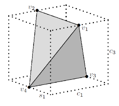
Figure 1: Shaded tetrahedron ${\cal T}$ embedded in a three-dimensional cube (dotted lines) is the domain of definition for the parameters (arguments) $s_{1}$, $c_{1}$, and $c_{3}$

This tetrahedron is enclosed in the three-dimensional cube $[-1,1]^{\otimes 3}$, has the vertices $v_{1}$, $v_{2}$, $v_{3}$, and $v_{4}$ and isosceles triangle faces. Volume of tetrahedron ${\cal T}$ equals one sixth part of cube volume ($=2^{3}$). So, one may say that the one-way deficit ${\rm\Delta}(s_{1},c_{1},c_{3})$ is a function on the tetrahedron ${\cal T}$.

Notice that the symmetric XXZ states (8) may be written in an equivalent form which is important for the MEMS problem IH00 ; HI00 ,

$$\rho_{AB}=q_{1}|\Psi^{+}\rangle\langle\Psi^{+}|+q_{2}|\Psi^{-}\rangle\langle\Psi^{-}|+q_{3}|00\rangle\langle 00|+q_{4}|11\rangle\langle 11|,$$ (11)

where $q_{1}+q_{2}+q_{3}+q_{4}=1$,

$$q_{1,2}=(1\pm 2c_{1}-c_{3})/4,\qquad q_{3,4}=(1\pm 2s_{1}+c_{3})/4,$$ (12)

$|\Psi^{\pm}\rangle=(|01\rangle\pm|10\rangle)/\sqrt{2}$ are the Bell states, and $|00\rangle$ and $|11\rangle$ are product-states orthogonal to $|\Psi^{\pm}\rangle$; they represent two “up” and “down” oriented spins (or two horizontally and vertically polarized photons), respectively. One may exchange $|\Psi^{+}\rangle\leftrightarrow|\Psi^{-}\rangle$ and $|00\rangle\leftrightarrow|11\rangle$ because they belong to the local unitary transformations and therefore do not change the value of quantum correlation. Quantities $q_{i}~{}(i=1,\cdots,4)$ are equal to the eigenvalues of density matrix and therefore must be non-negative. Hence the domain of definition in the space $(q_{1},q_{2},q_{3})$ is a three-dimensional corner restricted by four planes and conditions: $q_{1}\geq 0$, $q_{2}\geq 0$, $q_{3}\geq 0$, and $q_{1}+q_{2}+q_{3}\leq 1$. Further, a representation of Eq. (11) in Pauli matrices takes the form

$$\rho_{AB} =\frac{1}{4}\{1+(q_{1}+q_{2}+2q_{3}-1)(\sigma_{z}\otimes 1+1\otimes\sigma_{z})$$ (13)

$$+(q_{1}-q_{2})(\sigma_{x}\otimes\sigma_{x}+\sigma_{y}\otimes\sigma_{y})+[1-2(q_{1}+q_{2})]\sigma_{z}\otimes\sigma_{z}\}.$$

By the local unitary transformations, the state (11) is reduced to PABJWK04 ; APVW07

$$\rho_{AB}=q^{\prime}_{1}|\Phi^{+}\rangle\langle\Phi^{+}|+q^{\prime}_{2}|\Phi^{-}\rangle\langle\Phi^{-}|+q^{\prime}_{3}|01\rangle\langle 01|+q_{4}^{\prime}|10\rangle\langle 10|,$$ (14)

where $|\Phi^{\pm}\rangle=(|00\rangle\pm|11\rangle)/\sqrt{2}$ is the second pair of Bell states. The state (14) contains as a special case the Horodecki state KHJP10 which is a mixture of one Bell state and separable states orthogonal to the Bell one. Last, the class of maximally discordant mixed states (MDMS) having maximal quantum discord versus classical correlations is given by GGZ11

$$\rho_{AB}=\epsilon|\Phi^{+}\rangle\langle\Phi^{+}|+(1-\epsilon)(m|01\rangle\langle 01|+(1-m)|10\rangle\langle 10|)$$ (15)

($\epsilon$ and $m$ play a role of concentrations).

4 Formulas for branches

One-way quantum deficit for a bipartite state $\rho_{AB}$ is defined as the minimal increase of entropy after a von Neumann measurement on one party (without loss of generality, say, $B$) HHHOSSS05 (see also, e.g., MBCPV12 ; BDSRSS18 )

$${\rm\Delta}=\min_{\{\rm\Pi_{k}\}}S(\tilde{\rho}_{AB})-S(\rho_{AB}),$$ (16)

where $S(\cdot)$ means the von Neumann entropy and

$$\tilde{\rho}_{AB}\equiv\sum_{k}p_{k}\rho^{k}_{AB}=\sum_{k}(I\otimes{\rm\Pi}_{k})\rho_{AB}(I\otimes{\rm\Pi}_{k})^{+}$$ (17)

is the weighted average of post-measured states

$$\rho^{k}_{AB}=\frac{1}{p_{k}}(I\otimes{\rm\Pi}_{k})\rho_{AB}(I\otimes{\rm\Pi}_{k})^{+}$$ (18)

with the probabilities

$$p_{k}={\rm Tr}(I\otimes{\rm\Pi}_{k})\rho_{AB}(I\otimes{\rm\Pi}_{k})^{+}.$$ (19)

In Eq. (17), $\rm\Pi_{k}$ ($k=0,1$) are the general orthogonal projectors

$${\rm\Pi}_{k}=V\pi_{k}V^{+},$$ (20)

where $\pi_{k}=|k\rangle\langle k|$ and transformations $\{V\}$ belong to the special unitary group $SU(2)$. Rotations $V$ may be parametrized by two angles $\theta$ and $\phi$ (polar and azimuthal, respectively):

$$V=\left(\begin{array}[]{cc}\cos(\theta/2)&-e^{-i\phi}\sin(\theta/2)\\ e^{i\phi}\sin(\theta/2)&\cos(\theta/2)\end{array}\right)$$ (21)

with $0\leq\theta\leq\pi$ and $0\leq\phi<2\pi$.

Eigenvalues of matrix (9) are equal to

$$\lambda_{1,2}=(1\pm 2s_{1}+c_{3})/4,\qquad\lambda_{3,4}=(1\pm 2c_{1}-c_{3})/4.$$ (22)

Using these equations one gets the pre-measurement entropy function

$$S(s_{1},c_{1},c_{3})=h_{4}((1+2s_{1}+c_{3})/4,(1-2s_{1}+c_{3})/4,(1+2c_{1}-c_{3})/4,(1-2c_{1}-c_{3})/4),$$ (23)

where $h_{4}(x_{1},x_{2},x_{3},x_{4})=-x_{1}\log{x_{1}}-x_{2}\log{x_{2}}-x_{3}\log{x_{3}}-x_{4}\log{x_{4}}$ with condition $x_{1}+x_{2}+x_{3}+x_{4}=1$ is the quaternary entropy function. In explicit form,

$$S(s_{1},c_{1},c_{3})=2\ln 2$$

$$-\frac{1}{4}[(1+2c_{1}-c_{3})\ln(1+2c_{1}-c_{3})+(1-2c_{1}-c_{3})\ln(1-2c_{1}-c_{3})$$

$$+(1+2s_{1}+c_{3})\ln(1+2s_{1}+c_{3})+(1-2s_{1}+c_{3})\ln(1-2s_{1}+c_{3})].$$ (24)

The quantum state (9) after measurements ${\rm\Pi}_{k}$ ($k=0,1$) and averaging in accordance with Eq. (17) takes the form

$${\tilde{\rho}}_{AB}=\frac{1}{4}\!\left(\begin{array}[]{cccc}1+s_{1}+(s_{1}&\bullet&\bullet&\bullet\\ +c_{3})\cos^{2}\!\theta&&&\\ \\ \frac{1}{2}(s_{1}+c_{3})e^{i\phi}\sin\!2\theta&1-c_{3}+(s_{1}&\bullet&\bullet\\ &+c_{3})\sin^{2}\!\theta&&\\ \\ \frac{1}{2}c_{1}e^{i\phi}\sin\!2\theta&c_{1}\sin^{2}\!\theta&1-c_{3}-(s_{1}&\bullet\\ &&-c_{3})\sin^{2}\!\theta&\\ \\ c_{1}e^{2i\phi}\sin^{2}\!\theta&\ -\frac{1}{2}c_{1}e^{i\phi}\sin\!2\theta&\ \frac{1}{2}(s_{1}-c_{3})e^{i\phi}\sin\!2\theta&\ 1-s_{1}-(s_{1}\\ &&&-c_{3})\cos^{2}\!\theta\end{array}\right)$$ (25)

(for the sake of simplicity, the bold points are put instead of corresponding complex conjugated matrix elements of the Hermitian matrix ${\tilde{\rho}}_{AB}$).

We used the Mathematica software to extract the eigenvalues of matrix (25). First of all we established that the secular equation for the given matrix is factorized into product of two polynomials of second orders. In proving this key property, the following trick turned out useful. Namely, we first transformed the matrix elements to the exponential form (the command TrigToExp), found the secular equation, factorized it, then returned by applying the command ExpToTrig to the trigonometric expressions and finally simplified the result using the command FullSimplify. As a result, we arrived at the eigenvalues of post-measurement state (25),

$$\Lambda_{1,2}=\frac{1}{4}[\![1+s_{1}\cos\theta\pm\{(s_{1}+c_{3}\cos\theta)^{2}+c_{1}^{2}\sin^{2}\!\theta\}^{1/2}]\!],$$

(26)

$$\Lambda_{3,4}=\frac{1}{4}[\![1-s_{1}\cos\theta\pm\{(s_{1}-c_{3}\cos\theta)^{2}+c_{1}^{2}\sin^{2}\!\theta\}^{1/2}]\!].$$

It is seen that the azimuthal angle $\phi$ has dropped out from the given expressions. This is a general property and occurs every time when only one of the off-diagonals of the density matrix is non-zero VR12 ; MHR15 . Hence, the optimization reduces to that in a single variable $\theta$.

Using Eqs. (4) we find the post-measured entropy (entropy after measurement)

$$\tilde{S}(\theta)\equiv S(\tilde{\rho}_{AB})=h_{4}(\Lambda_{1},\Lambda_{2},\Lambda_{3},\Lambda_{4}),$$ (27)

where $h_{4}(\cdot)$ is again the quaternary entropy function. The function $\tilde{S}$ of argument $\theta$ is invariant under the transformation $\theta\to\pi-\theta$ therefore it is enough to restrict oneself by values of $\theta\in[0,\pi/2]$. Moreover, the pre- and post-measured entropies $S$ and $\tilde{S}$, as functions of $s_{1}$ and $c_{1}$, are symmetric under the reflections $s_{1}\to-s_{1}$ and $c_{1}\to-c_{1}$.

Notice the following. The post-measument entropy $\tilde{S}$ is related to the conditional entropy $S_{cond}$ [see Eqs. (25)-(26) in Ref. Y17 ] by equation (see SXL13 and also Appendix in Ref. Y17 )

$$\tilde{S}(\theta)=S_{cond}(\theta)+h((1+s_{1}\cos\theta)/2),$$ (28)

with $h(x)=-x\ln x-(1-x)\ln(1-x)$ being Shennon’s binary entropy function. The first derivative of $h$-term with respect to $\theta$ equals zero at both endpoints $\theta=0$ and $\pi/2$. Hence if the first derivative of $S_{cond}(\theta)$ with respect to $\theta$ vanishes at $\theta=0$ and $\pi/2$ then the same takes place for the post-measured entropy $\tilde{S}(\theta)$ and vice versa. Moreover, in accordance with Eq. (28), the non-optimized one-way deficit can be written as

$$\Delta(\theta)=h((1+s_{1}\cos\theta)/2)-S(\rho_{AB})+S_{cond}(\theta).$$ (29)

On the other hand, the measurement-dependent quantum discord can be presented as

$$Q(\theta)=h((1+s_{1}\cos\theta)/2)|_{\theta=0}-S(\rho_{AB})+S_{cond}(\theta)$$ (30)

because $h((1+s_{1}\cos\theta)/2)|_{\theta=0}=S(\rho_{B})$, where $\rho_{B}={\rm Tr}_{A}\rho_{AB}$. So, Eqs. (29) and (30) show a very close mathematical relation between both measures of quantum correlation: the only difference is either we take $h$-term with arbitrary $\theta$ or set $\theta=0$. This relation is valid for general X states.

From Eqs. (4) and (27), one gets an expression for the post-measurement entropy:

$$\tilde{S}(\theta;s_{1},c_{1},c_{3})=2\ln 2$$

$$-\frac{1}{4}\sum_{m,n=1}^{2}\biggl{(}1+(-1)^{m}s_{1}\cos\theta+(-1)^{n}\sqrt{(s_{1}+(-1)^{m}c_{3}\cos\theta)^{2}+c_{1}^{2}\sin^{2}\theta}\biggr{)}$$

$$\times\ln\biggl{(}1+(-1)^{m}s_{1}\cos\theta+(-1)^{n}\sqrt{(s_{1}+(-1)^{m}c_{3}\cos\theta)^{2}+c_{1}^{2}\sin^{2}\theta}\biggr{)}.$$ (31)

In the following analysis, this function will serve us to probe and identify the types of subregions in phase diagrams. The function $\tilde{S}(\theta;s_{1},c_{1},c_{3})$ is differentiable at any point $\theta$ and, in full conferment with the statement made in the Introduction, its first derivatives with respect to $\theta$ identically equal zero for $\forall\,s_{1},c_{1},c_{3}\in{\cal T}$ at both ends of the interval $[0,\pi/2]$.

The post-measurement entropy at the endpoint $\theta=0$ is given as

$$\tilde{S}_{0}\equiv\tilde{S}(0)=2\ln 2-\frac{1}{2}(1-c_{3})\ln(1-c_{3})$$

$$-\frac{1}{4}[(1+2s_{1}+c_{3})\ln(1+2s_{1}+c_{3})+(1-2s_{1}+c_{3})\ln(1-2s_{1}+c_{3})]$$ (32)

and at the endpoint $\theta=\pi/2$:

$$\tilde{S}_{\pi/2}\equiv\tilde{S}(\pi/2)=2\ln 2-\frac{1}{2}\biggl{[}\biggl{(}1+\sqrt{s_{1}^{2}+c_{1}^{2}}\biggr{)}\ln\biggl{(}1+\sqrt{s_{1}^{2}+c_{1}^{2}}\biggr{)}$$

$$+\biggl{(}1-\sqrt{s_{1}^{2}+c_{1}^{2}}\biggr{)}\ln\biggl{(}1-\sqrt{s_{1}^{2}+c_{1}^{2}}\biggr{)}\biggr{]}.$$ (33)

Equations (23),(4), and (27) define the measurement-dependent one-way deficit function

$$\Delta(\theta)={\tilde{S}}(\theta)-S.$$ (34)

In the wake of ${\tilde{S}}(\theta)$, the first derivative of $\Delta(\theta)$ with respect to $\theta$ is identically equal to zero at both endpoints $\theta=0$ and $\theta=\pi/2$:

$${\tilde{S}}^{\prime}(0)=\Delta^{\prime}(0)\equiv 0,\qquad{\tilde{S}}^{\prime}(\pi/2)=\Delta^{\prime}(\pi/2)\equiv 0.$$ (35)

By analogy with the quantum discord Y14 ; Y14a ; MHR15 ; Y15 (see also Y17 ), the one-way quantum deficit may be written as almost closed analytical formula Y18

$$\rm\Delta=\min\{\Delta_{0},\Delta_{\pi/2},\Delta_{\vartheta}\}.$$ (36)

Thus, it can consist of three branches. However, it should be noted that in general these branches may further out split into new subbranches.

Using the above equations one obtains the expression for the 0-branch:

$$\Delta_{0}(s_{1},c_{1},c_{3})=-\frac{1}{2}(1-c_{3})\ln(1-c_{3})$$

$$+\frac{1}{4}[(1+2c_{1}-c_{3})\ln(1+2c_{1}-c_{3})+(1-2c_{1}-c_{3})\ln(1-2c_{1}-c_{3})].$$ (37)

Surprisingly, this branch is identical to the similar branch of discord $Q_{0}$ Y17 , i.e., $\Delta_{0}=Q_{0}$. Moreover the function $\Delta_{0}$ is symmetric under the reflection $c_{1}\to-c_{1}$ and does not depend on $s_{1}$.

For the branch $\Delta_{\pi/2}$ with the $\pi/2$ optimal measured angle, we have

$$\Delta_{\pi/2}(s_{1},c_{1},c_{3})=-\frac{1}{2}\biggl{[}\biggl{(}1+\sqrt{s_{1}^{2}+c_{1}^{2}}\biggr{)}\ln\biggl{(}1+\sqrt{s_{1}^{2}+c_{1}^{2}}\biggr{)}$$

$$+\biggl{(}1-\sqrt{s_{1}^{2}+c_{1}^{2}}\biggr{)}\ln\biggl{(}1-\sqrt{s_{1}^{2}+c_{1}^{2}}\biggr{)}\biggr{]}$$

$$+\frac{1}{4}[(1+2c_{1}-c_{3})\ln(1+2c_{1}-c_{3})+(1-2c_{1}-c_{3})\ln(1-2c_{1}-c_{3})$$

$$+(1+2s_{1}+c_{3})\ln(1+2s_{1}+c_{3})+(1-2s_{1}+c_{3})\ln(1-2s_{1}+c_{3})].$$ (38)

This function is symmetric both on $s_{1}$ and $c_{1}$.

The third and last branch $\Delta_{\vartheta}$ is obtained by numerically solving the one-dimensional optimization problem for the function $\tilde{S}(\theta)$.

We turn now to the discussion of boundaries distinguishing the phases of quantum correlation.

5 Equations for boundaries

The problem of phases and boundaries between them is well known in thermodynamics and statistical physics B82 ; LL_StPh as well as in other fields of science. Classification of phases depends on characteristic features which are put in its ground. Therefore it is not surprising that, e.g., one discovers more and more new phases for water.

Quantum correlations are piecewise-defined functions. A choice of a certain branch in the given point of parameter space is dictated by a minimum condition like (36). But how to decompose the whole domain of definition of quantum correlation function into subdomains? The answer to this question was firstly given in Refs. Y14 ; Y14a (see also MHR15 ; Y15 ) with the quantum discord.

Applying those ideas to the one-way quantum deficit, one may say the following. On the one hand, the boundary between the phases with zero and $\pi/2$ optimal measurement angles is controlled by the equilibrium condition

$$\tilde{S}_{0}=\tilde{S}_{\pi/2}\quad{\rm or}\quad\Delta_{0}=\Delta_{\pi/2}.$$ (39)

When crossing this boundary, the optimal measurement angle experiences the jump $\Delta\vartheta=\pi/2$.

On the other hand, the transitions from the $\vartheta$-phase to the 0- or $\pi/2$-one can occur via a bifurcation of minimum of the post-measurement entropy function at the endpoints $\theta=0$ and $\pi/2$. In these cases the equations for the boundaries are reduced to a requirement of vanishing the second derivatives of post-measurement entropy or measurement-dependent one-way deficit with respect to $\theta$ at corresponding endpoints YWF16 ; Y18

$$\tilde{S}^{\prime\prime}(0)=0\quad{\rm or}\quad\Delta^{\prime\prime}(0)=0\quad$$ (40)

for the 0-boundary and

$$\tilde{S}^{\prime\prime}(\pi/2)=0\quad{\rm or}\quad\Delta^{\prime\prime}(\pi/2)=0$$ (41)

for the $\pi/2$-one. Here the optimal measurement angle jumps equal $\Delta\vartheta=0$.

For the quantum states under discussion the second derivatives at endpoints follow from Eq. (4) and equal

$$\tilde{S}^{\prime\prime}(0)= \frac{1}{4}\biggl{\{}s_{1}\ln\frac{1+2s_{1}+c_{3}}{1-2s_{1}+c_{3}}+c_{3}\ln\frac{(1+2s_{1}+c_{3})(1-2s_{1}+c_{3})}{(1-c_{3})^{2}}$$ (42)

$$-c_{1}^{2}\biggl{[}\frac{1}{s_{1}+c_{3}}\ln\frac{1+2s_{1}+c_{3}}{1-c_{3}}+\frac{1}{s_{1}-c_{3}}\ln\frac{1-c_{3}}{1-2s_{1}+c_{3}}\biggr{]}\biggl{\}}$$

and

$$\tilde{S}^{\prime\prime}(\pi/2)=c_{1}^{2}\frac{s_{1}^{2}+c_{1}^{2}-c_{3}^{2}}{2r^{3}}\ln\frac{1+r}{1-r}-\frac{1}{2}s_{1}^{2}\biggl{(}\frac{(1+c_{3}/r)^{2}}{1+r}+\frac{(1-c_{3}/r)^{2}}{1-r}\biggr{)}$$ (43)

with $r=\sqrt{s_{1}^{2}+c_{1}^{2}}$.

Equations (39), (40), and (41) together with expressions (4), (4), (4), (4), (42), and (43) are transcendental and they can be solved numerically by the bisection method.

The above mechanism of arising the boundaries between phases is confirmed for the cases when the post-measurement entropy function is unimodal. However, most recently Y18 a bimodal behavior for the post-measurement entropy function has been found and a new important equation has been added to the collection of boundary equations, namely

$$\tilde{S}_{0}=\tilde{S}_{\vartheta}\quad{\rm or}\quad\Delta_{0}=\Delta_{\vartheta}.$$ (44)

These conditions reflect a jump (sudden change) of optimal measurement angle from zero to a finite step $\Delta\vartheta>0$ but $\Delta\vartheta\neq\pi/2$. For definiteness, we will call such a boundary as the 0^′-one.

Generally speaking the jumps between the endpoint $\theta=\pi/2$ and global interior minimum are possible theoretically but up to the present they were not met in our practice.

Note for a reference that we solved the equations (44) for the 0^′-boundary also by the bisection method with searching the interior minimum of post-measurement entropy or measurement-dependent one-way quantum deficit at every step of iteration procedure by the golden section method.

The above classification of phases is based on the type of optimal measurement angle. But in general such an approach does not exhaust all possible branches of piecewise-defined function. New subbranches can appear from the splitting of some original branches. For instance, such a phenomenon was previously observed for the $\pi/2$-branch of discord, $Q_{\pi/2}$, which decays into two subbranches $Q_{\pi/2}^{(1)}$ and $Q_{\pi/2}^{(2)}$ in the limit of Bell-diagonal states (see Fig. 7b in Ref. Y15 and Sec. 2.1 in Ref. Y17 ). The reason is simple: when $s_{1}=s_{2}=0$, the function $Q_{\pi/2}(c_{1},c_{2},c_{3})$ by $|c_{1}|\neq|c_{2}|$ contains inside itself the piecewise functions like $|c_{1}-c_{2}|$. In similar situations, the additional boundaries are revealed from the detection of fracture points, i.e., from the condition of discontinuity for the first derivatives with respect to the parameters of the model:

$${\rm\Delta}_{x}^{\prime}(x-0)\neq{\rm\Delta}_{x}^{\prime}(x+0),\quad x\in\{s_{1},c_{1},c_{3}\}.$$ (45)

However, we did not observe such cases in the present paper because $c_{1}=c_{2}$.

6 Phase diagram for the symmetric XXZ state

The task now is to separate the body $\cal T$ by using boundary equations into subdomains each one corresponding to a certain branch according to the minimum condition (36). Our strategy is reduced to the following. We will take different two-dimensional sections of tetrahedron $\cal T$, solve the equations for boundaries, and then visually analyze the shapes of curves $\tilde{S}(\theta)$ or $\Delta(\theta)$. The position of global minimum of these curves will give us the answer to the question about the type of branch in the given part of section.

The one-way deficit function ${\rm\Delta}(s_{1},c_{1},c_{3})$ is invariant under the transformations $s_{1}\to-s_{1}$ and $c_{1}\to-c_{1}$. Hence the body $\cal T$ with all subdomains is symmetric relative to the mirror reflections in the planes $s_{1}=0$ and $c_{1}=0$. Owing to this, it is enough to study the phases only in a quarter of tetrahedron $\cal T$.

6.1 Phase diagrams on faces

We begin the analysis with the faces of tetrahedron $\cal T$. Due to the mirror symmetry, it is enough to study the phases only on two adjacent semi-faces. Without loss of generality, we consider the faces $v_{1}v_{2}v_{4}$ and $v_{1}v_{3}v_{4}$ (see Fig. 1). Both halves of these two adjacent faces are shown in Fig. 2 in an unfolded form.

Figure 2: Phase diagram of one-way quantum deficit on the faces of tetrahedron $\cal T$. The diagonal dotted line $v_{1}v_{4}$ dividing the figure area in two triangle parts is the corresponding edge of the tetrahedron. The upper triangle is a half of the face $v_{1}v_{2}v_{4}$ while the lower one is a half of the face $v_{1}v_{3}v_{4}$. (The latter represents the phase diagram Y18 in new variables.) The points “a” and “b” lie on the diagonal $v_{1}v_{4}$, their coordinates $(c_{1},c_{3})$ being equal $(-0.5,0)$ and $(-0.675151,-0.350302)$, respectively, whereas the point “c” is located at $(-0.709723,-0.538191)$

Consider first the upper triangle. Here $c_{1}=-(1-c_{3})/2$. Solution of equations from the previous section leads to the curves labeled in Fig. 2 by symbols 0 and 1 which correspond to the 0- and $\pi/2$-boundaries, respectively. Testing the different parts of triangle by the shape of curve $\tilde{S}(\theta)$ allows to identify the types of separate subdomains; they are marked in Fig. 2 by corresponding names of branches. Three found types of post-measurement entropy shapes (monotonically decreasing, unimodal, and monotonically increasing) are illustrated in Fig. 3.

Figure 3: Evolution of post-measurement entropy shapes by pass along the line $c_{3}=0.15$ on the face $v_{1}v_{2}v_{4}$ [i.e, when $c_{1}=(1-c_{3})/2$)] for $s_{1}=0.2$ (a), 0.406975 (b), 0.44 (c), and 0.483997 (c). Cases (b) and (d) correspond to the moments of bifurcations of minimum which occur on the boundary curves 1 and 0, respectively

More complicated shapes of $\tilde{S}(\theta)$ are absent on this face.

Phase diagram on the lower triangle part of Fig. 2 [here $s_{1}=(1+c_{3})/2$] corresponds to the case which has been considered in Ref. Y18  (Fig. 7 there); the only difference is the coordinates $(c_{1},c_{3})$ instead $(q_{1},q_{2})$. Here the bimodal behavior of $\tilde{S}(\theta)$ takes place and, correspondingly, the $0^{\prime}$-boundary on which the optimal measurement angle discontinuously changes its value exists between the points “a” and “c”. The curve $0^{\prime}$ is a line of continuously varying $\Delta\vartheta$ in the limits from 0 to $\pi/2$ (see Table 1 in Y18 ). The critical line 2 corresponds to the boundary when $\Delta_{0}=\Delta_{\pi/2}$.

It is interesting to compare the location of phases $\Delta_{0}$, $\Delta_{\pi/2}$, and $\Delta_{\vartheta}$ in the tetrahedron $\cal T$ with that of similar discord phases $Q_{0}$, $Q_{\pi/2}$, and $Q_{\theta^{*}}$ found earlier for the same quantum states Y17 . One can see the phases of one-way deficit and discord on faces of $\cal T$ in Fig. 4.

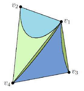
Figure 4: (Color online) An outward appearance of tetrahedron $\cal T$ for the one-way deficit (left, see also Fig. 2) and discord (right). The regions $\Delta_{0}$ and $Q_{0}$ are shown by the blue color while the $\Delta_{\pi/2}$ and $Q_{\pi/2}$ ones are shown by the green color. The region $\Delta_{\vartheta}$ is yellow-colored and because the region $Q_{\theta^{*}}$ lies inside the tetrahedron it is not seen

Because the one-way quantum deficit must be identical to the quantum discord for the Bell-diagonal states, we satisfy ourselves that really ${\rm\Delta}=Q$ in the case $s_{1}=0$. More and above, we observe that, due to the equality $\Delta_{0}=Q_{0}$, the one-way deficit $\rm\Delta$ and discord $Q$ are equal when the $\Delta_{0}$ and $Q_{0}$ regions coincide. This circumstance considerably enlarges the common part of total domain $\cal T$, where both measures of quantum correlation yield the same result.

6.2 Phase diagrams inside the tetrahedron $\cal T$

Consider now the phase structure in the interior of tetrahedron. The study will be performed by scanning the body $\cal T$ by taking cross-sections with planes $c_{3}=const$. We will go from the top to the bottom of the tetrahedron.

When $c_{3}=1$, i.e., on the edge $v_{1}v_{2}$, all quantum correlations vanish because here $c_{1}=0$ and the system is purely classical.

In the subsequent investigation it will be convenient to consider five separate intervals for $c_{3}$ taking into account the variation of phases in longitudinal direction (see Fig. 2).

First of all the calculations show that the one-way deficit equals ${\rm\Delta}=\Delta_{0}$ in the band $1/3\leq c_{3}\leq 1$.

By $c_{3}<1/3$, the other two phases appear in the slices. Typical phase diagram for the one-way deficit in the interval of $c_{3}$ from 1/3 to 0 is shown in Fig. 5a for the cross-section $c_{3}=0.1$.

Figure 5: Phase diagrams of one-way deficit (a) and discord (b) by $c_{3}=0.1$. Subregions $\Delta_{\vartheta}$ lie between the pairs of solid lines in a graph (a). Similar subregions for the quantum discord, $Q_{\theta^{*}}$, are thin too and therefore their locations are shown only schematically by double solid-dotted lines in a graph (b) (see also Fig. 3 in Y17 )

Phase diagram for the discord is shown in Fig. 5b for a comparison. One sees the significant differences between both measures of quantum correlation. However they are the same on the line $s_{1}=0$ (Bell’s case) and in common parts of regions $\Delta_{0}$ and $Q_{0}$.

Because the phase diagrams in cross-sections are symmetric about the $s_{1}$ and $c_{1}$ axes, one may only focus on a quarter of the diagram. Moreover, as calculations show, the boundaries between phases of one-way deficit lie in the regions $c_{1}\geq|c_{3}|$ therefore it is enough to restrict oneself by the strips $|c_{3}|\leq c_{1}\leq(1-c_{3})/2$. Left part of Fig. 6 shows the subregion by $c_{3}=0.1$ in detail.

Figure 6: Fragments of phase diagrams in the sections $c_{3}=0.1$ (on the left) and $c_{3}=0$ (on the right). The curves 0 represent the 0-boundaries while the lines 1 are the $\pi/2$-ones

The boundaries 1 and 0 end on the upper edge of cross-section rectangle at the points with abscissas $s_{1}=0.416297$ and 0.502469, respectively. The area of the $\Delta_{\vartheta}$ segment equals 0.008639 in the absolute units. Hence the relative area of the whole $\Delta_{\vartheta}$ region to the area of cross-section rectangle is 3.5%. The similar area for the discord $Q_{\theta^{*}}$ equals 5.5$\times 10^{-5}$% only. So, one may ascertain that the region with state-dependent optimal measurement angle is experimentally accessible for the one-way deficit but not for the discord.

Phase diagram in the cross-section $c_{3}=0$ is also depicted in Fig. 6. The boundary 0 has reached here the right upper corner of the cross-section rectangle, i.e., the vertex with coordinates $(0.5,0.5)$. As follow from Eqs. (40) and (42), the 0-boundary is reduced here to the straight lines $c_{1}=s_{1}$. The endpoint of $\pi/2$-boundary lies at $s_{1}=0.415037$ on the upper edge of the cross-section rectangle. The relative area of the fraction $\Delta_{\vartheta}$ achieves now 4.2%.

The third interval of $c_{3}$ ranges from $c_{3}=0$ to $c_{3}=-0.350302$, i.e., up to the point when the $\pi/2$-boundary reaches the vertex of section rectangle (this corresponds to a segment from the point “a” to the point “b” in Fig. 2). Characteristic phase diagram in these transverse slices is drawn in Fig. 7.

Figure 7: Phase diagram by $c_{3}=-0.2$ (a) and its fragment (b). The 0-boundary is partly replaced by the $0^{\prime}$-boundary. The arrows on the right vertical sides ($s_{1}=0.4$) mark the point $c_{1}=0.576208$ which corresponds to the endpoint of the $0^{\prime}$-boundary

Near the vertical edge of section rectangle, the 0-boundary is here replaced by $0^{\prime}$-boundary, i.e., instead of the appearance of interior minimum via bifurcation, there is now observed a bimodal behavior of curve $\tilde{S}(\theta)$ (see Fig. 8) that is accompanied with the discontinuous change of optimal measurement angle on the critical line $0^{\prime}$.

Figure 8: Post-measurement entropy $\tilde{S}$ vs $\theta$ by $c_{3}=-0.2$, $c_{1}=0.576208$, and $s_{1}=0.4$ (a) and 0.39995 (b). Both dependencies exhibit the bimodal behavior

Figure 8a fixes the moment when the interior minimum achieves the value of post-measurement entropy at the angle $\theta=0$. Between the lines 0 and 0^′ the interior minimum is lower than the minimum at $\theta=0$ as shown in Fig. 8b; hence the fraction $\Delta_{\vartheta}$ exists here.

The next interval $-0.538191<c_{3}<-0.350302$ corresponds to a part of tetrahedron between the points “b” and “c” shown in Fig. 2. Phase diagram by $c_{3}=-0.4$ is presented in Fig. 9.

Figure 9: Phase diagram in the cross-section $c_{3}=-0.4$ (a) and its piece near the vertical edge of cross rectangle (b). The arrow marks the point $c_{1}=0.652165$ of $0^{\prime}$-boundary on the line $s_{1}=0.3$

As $c_{3}$ reaches the value of $-0.538191$, the endpoints of curves 1 and $0^{\prime}$ meet each other on the side $s_{1}=(1+c_{3})/2$.

By further decreasing the value of $c_{3}$, the $\pi/2$- and $0^{\prime}$-lines intersect inside the body $\cal T$ and the boundary $\Delta_{0}=\Delta_{\pi/2}$ appears (see Fig. 10).

Figure 10: Phase diagram by $c_{3}=-0.6$ (a) and its part (b). The lines 1 and $0^{\prime}$ correspond respectively to the $\pi/2$- and $0^{\prime}$-boundaries while the line 2 is the $\Delta_{0}=\Delta_{\pi/2}$ boundary. The fraction $\Delta_{\vartheta}$ lies between the critical lines 1 and $0^{\prime}$. Black circle is a triple point

The post-measured entropy curve near the critical line 2 has the interior maximum.

In the limit $c_{3}\to-1$, i.e., on the edge $v_{3}v_{4}$ of tetrahedron ${\cal T}$, the value of parameter $s_{1}$ vanishes, the region $\Delta_{\vartheta}$ disappears, and the quantum state transforms into the Bell-diagonal one. On this edge the optimized one-way deficit and discord coincide and are given by

$${\rm\Delta}=Q=\frac{1}{2}[(1+c_{1})\ln(1+c_{1})+(1-c_{1})\ln(1-c_{1})].$$ (46)

In the middle of the edge, $c_{1}=0$, the quantum correlation is zero while at the vertecies $v_{3}$ and $v_{4}$ ($c_{1}=\pm 1$) it is, vice versa, maximal and equals 1 bit.

7 Conclusions and outlook

In this paper we have investigated the three-dimensional phase diagram of one-way quantum deficit for the XXZ family of symmetric X quantum states. The set of Figs. 2, 4, 5, 6, 7, 9, and 10 provides insight into a complete picture of all typical features in the phase diagram. It is probable that an application of technologies like holography or virtual reality would be suitable for the visualization of such 3D diagrams.

It has been established that there are three branches of one-way deficit function and hence three different subdomains corresponding them. Two of which, $\Delta_{0}$ and $\Delta_{\pi/2}$, are characterized by constant measurement angles — zero and $\pi/2$, respectively. At the same time, the third region $\Delta_{\vartheta}$ is characterized by non-universal behavior of optimal measurement angle $\vartheta$ because it continuously varies with the parameters of density matrix.

We have found that three possible regions of one-way deficit can be separated by four kinds of boundaries: 0 or 0^′ which divide the $\Delta_{0}$ and $\Delta_{\vartheta}$ fractions, $\pi/2$ that exists between $\Delta_{\pi/2}$ and $\Delta_{\vartheta}$ phases, and lastly the $\Delta_{0}=\Delta_{\pi/2}$ boundary between regions $\Delta_{0}$ and $\Delta_{\pi/2}$. The optimal measurement angle $\vartheta$ is continuous when crossing the 0- and $\pi/2$-boundaries, whereas it experiences the jump $\Delta\vartheta=\pi/2$ by going across the $\Delta_{0}=\Delta_{\pi/2}$ boundary and varies in the limits from zero to $\pi/2$ on the critical line 0^′.

A comparison of behavior of the one-way quantum deficit and discord shows quantitative and qualitative difference between those measures of quantum correlation in general. However they are identical for the Bell-diagonal states, i.e., in the plane $s_{1}=0$. Moreover, we have established that both measures of quantum correlation coincide in the intersection of regions $\Delta_{0}$ and $Q_{0}$ ($\Delta_{0}\cap Q_{0}$). (This result is valid for general X states.) But quite a difference in other cases allows to say that the named quantities represent different kinds of quantum correlation. This situation is similar to the one taking place for the mean value of numbers and its various types: the arithmetic mean, harmonic mean, and so on. By this, each kind of mean has its own application.

We have discovered that the region with variable optimal measurement angle is in several orders larger for the one-way quantum deficit in comparison with the quantum discord.

It should be noted that all quantum correlations are certain functions of ordinary statistical correlations (2) [see, e.g., Eqs. (4) or (4)]. This is a sequence of the fact that any quantum correlation is defined by the system density matrix but its entries are expressed through the statistical correlation functions.

We have restricted ourselves only by one phase diagram of full atlas. The work started here should be continued to cover by separate diagrams the total seven-dimensional space of X-state parameters.

Acknowledgment I am grateful to Dr. A. I. Zenchuk for his valuable remarks.

References

- (1) Modi, K., Brodutch, A., Cable, H., Paterek, T., Vedral, V.: The classical-quantum boundary for correlations: discord and related measures. Rev. Mod. Phys. 84, 1655 (2012)
- (2) Streltsov, A.: Quantum correlations beyond entanglement and their role in quantum information theory. Springer, Berlin (2015)
- (3) Adesso, G., Bromley, T.R., Cianciaruso, M.: Measures and applications of quantum correlations. J. Phys. A: Math. Theor. 49, 473001 (2016)
- (4) Lectures on general quantum correlations and their applications. Eds: Fanchini, F.F., Soares-Pinto, D.O., Adesso, G. Springer, Berlin (2017)
- (5) Bera, A., Das, T., Sadhukhan, D., Roy, S.S., Sen(De), A., Sen, U.: Quantum discord and its allies: a review of recent progress. Rep. Prog. Phys. 81, 024001 (2018)
- (6) Oppenheim, J., Horodecki, M., Horodecki, P., Horodecki, R.: Thermodynamical approach to quantifying quantum correlations. Phys. Rev. Lett. 89, 180402 (2002)
- (7) Horodecki, M., Horodecki, K., Horodecki, P., Horodecki, R., Oppenheim, J., Sen(De), A., Sen, U.: Local information as a resource in distributed quantum systems. Phys. Rev. Lett. 90, 100402 (2003)
- (8) Horodecki, M., Horodecki, P., Horodecki, R., Oppenheim, J., Sen(De), A., Sen, U., Synak-Radtke, B.: Local versus nonlocal information in quantum-information theory: Formalism and phenomena. Phys. Rev. A 71, 062307 (2005)
- (9) Zurek, W.H.: Quantum discord and Maxwell’s demons. Phys. Rev. A 67, 012320 (2003)
- (10) Ye, B.-L., Fei, S.-M.: A note on one-way quantum deficit and quantum discord. Quantum Inf. Process. 15, 279 (2016)
- (11) Ciliberti, L., Rossignoli, R., Canosa, N.: Quantum discord in finite chains. Phys. Rev. A 82, 042316 (2010)
- (12) Vinjanampathy, S., Rau, A.R.P.: Quantum discord for qubit-qudit systems. J. Phys. A: Math. Theor. 45, 095303 (2012)
- (13) Huang, Y.: Quantum discord for two-qubit states: Analytical formula with very small worst-case error. Phys. Rev. A 88, 014302 (2013)
- (14) Ye, B.-L., Wang, Y.-K., Fei, S.-M.: One-way quantum deficit and decoherence for two-qubit states. Int. J. Theor. Phys. 55, 2237 (2016)
- (15) Yurischev, M.A.: Extremal properties of conditional entropy and quantum discord for XXZ, symmetric quantum states. Quantum Inf. Process. 16:249 (2017)
- (16) Brodutch, A., Modi, K.: Criteria for measures of quantum correlations. Quantum Inf. Comput. 12, 0721 (2012)
- (17) Yurischev, M.A.: Quantum discord for general X and CS states: a piecewise-analytical-numerical formula. ArXiv:1404.5735v1 [quant-ph]
- (18) Yurishchev, M.A.: NMR dynamics of quantum discord for spin-carrying gas molecules in a closed nanopore. J. Exp. Theor. Phys. 119, 828 (2014), arXiv:1503.03316v1 [quant-ph]
- (19) Postnikov, M.M.: Lectures in geometry. Semester III. Smooth manifolds. Nauka, Moscow (1987), lecture 6 [in Russian]
- (20) Baxter, R.J.: Exactly solved models in statistical mechanics. Academic, London (1982)
- (21) Fendley, P.: Modern statistical mechanics. The university of Virginia (2014)
- (22) Barbieri, M., De Martini, F., Di Nepi, G., Mataloni, P.: Generation and characterization of Werner states and maximally entangled mixed states by a universal source of entanglement. Phys. Rev. Lett. 92, 177901 (2004)
- (23) Mendonca, P.E.M.F, Marchiolli, M.A., Hedemann, S.R.: Maximally entangled mixed states for qubit-qutrit systems. Phys. Rev. A 95, 022324 (2017)
- (24) Ishizaka, S., Hiroshima, T.: Maximally entangled mixed states under nonlocal unitary operations in two qubits. Phys. Rev. A 62, 022310 (2000)
- (25) Hiroshima, T., Ishizaka, S.: Local and nonlocal properties of Werner states. Phys. Rev. A 62, 044302 (2000)
- (26) Peters, N.A., Altepeter, J.B., Branning, D., Jeffrey, E.R., Wei, T.-C., Kwiat, P.G.: Maximally entangled mixed states: creation and concentration. Phys. Rev. Lett. 92, 133601 (2004); Erratum in: Phys. Rev. Lett. 96, 159901 (2006)
- (27) Aiello, A., Puentes, G., Voigt, D., Woerdman, J.P.: Maximally entangled mixed-state generation via local operations. Phys. Rev. A 75, 062118 (2007)
- (28) Kim, H., Hwang, M.-R., Jung, E., Park, D.K.: Difficulties in analytic computation for relative entropy of entanglement. Phys. Rev. A 81, 052325 (2010)
- (29) Galve, F., Giorgi, G.L., Zambrini, R.: Maximally discordant mixed states of two qubits. Phys. Rev. A 83, 012102 (2011); Erratum in: Phys. Rev. A 83, 069905 (2011)
- (30) Maldonado-Trapp, A., Hu, A., Roa, L.: Analytical solutions and criteria for the quantum discord of two-qubit X-states. Quantum Inf. Process. 14, 1947 (2015)
- (31) Shao, L.-H., Xi, Z.-J., Li, Y.M.: Remark on the one-way quantum deficit for general two-qubit states. Commun. Theor. Phys. 59, 285 (2013)
- (32) Yurischev, M.A.: On the quantum discord of general X states. Quantum Inf. Process. 14, 3399 (2015)
- (33) Yurischev, M.A.: Bimodal behavior of post-measured entropy and one-way quantum deficit for two-qubit X states. Quantum Inf. Process. 17:6 (2018)
- (34) Landau, L.D., Lifshitz, E.M.: Statistical physics. Part 1. Fizmatlit, Moscow (2005) [in Russian], Pergamon, Oxford (1980) [in English]