Graph Matching with Anchor Nodes: A Learning Approach

Abstract

In this paper, we consider the weighted graph matching problem with partially disclosed correspondences between a number of anchor nodes. Our construction exploits recently introduced node signatures based on graph Laplacians, namely the Laplacian family signature (LFS) on the nodes, and the pairwise heat kernel map on the edges. In this paper, without assuming an explicit form of parametric dependence nor a distance metric between node signatures, we formulate an optimization problem which incorporates the knowledge of anchor nodes. Solving this problem gives us an optimized proximity measure specific to the graphs under consideration. Using this as a first order compatibility term, we then set up an integer quadratic program (IQP) to solve for a near optimal graph matching. Our experiments demonstrate the superior performance of our approach on randomly generated graphs and on two widely-used image sequences, when compared with other existing signature and adjacency matrix based graph matching methods.

1 Introduction

The exact and approximate graph matching problem is of great interest in computer vision due to its numerous applications in areas such as 2D and 3D image registration, object recognition and biomedical identification, and object tracking in video sequences. An important variant of the problem is the semi-supervised setting where a small proportion of correct node correspondences between the graphs are known. Such correspondences can be based on additional information provided for only a few nodes, human judgement or prior knowledge, etc. Algorithms that can take advantage of this information to infer the correspondences for the rest of the graph nodes are highly desirable.

While there has been a recent effort in applying machine learning concepts to the graph matching problem in computer vision [3, 15], these works are based on the assumption that a training set consisting of pairs of graphs with fully correct correspondences given, and that the training set is representative enough of testing graphs, so that learning done with training graphs can be usefully transferred to testing graphs. This problem setup, however, is different from our setting where we only have two graphs with partially known correspondences; in a sense, these known correspondences constitute our “training data”. In addition, this amounts to a much smaller and more restricted amount of training data, making the problem challenging.

In this work we provide a method for effectively incorporating known correspondences into the commonly used integer quadratic program formulation of graph matching. Specifically, our main contribution is to devise a new first order compatibility term between two nodes of different graphs. Our method uses the recently proposed one-parameter family of node signatures called Laplacian Family Signatures (LFS) [11], which provide a feature vector (signature) for each node based solely on the node’s structural position within the graph. In contrast to [11], we do not assume an explicit form of parametric dependence for generating these signatures, but leave it in an unspecified generic form. Since graph matching is performed using the dissimilarity/distance between these signatures, we derive the distance between the generic signatures. As a result of this manipulation, we find that the entire process of computing and comparing these generic signatures can be encoded into a single proximity matrix. We then introduce an algorithm to learn this proximity matrix from the knowledge of provided correct correspondences. This is done by requiring anchor nodes in one graph to correspond near to their known partners in the other and to be far from non-correspondences, which can be set up as a max-margin problem [28].

This method was chosen due to a number of benefits. First, our max-margin formulation makes an effective use of the scarce training data: even a small number of known correspondences (two anchor correspondences are used in all of our experiments) leads to a large number of constraints on the proximity matrix. Second, our formulation results in learning a proximity matrix that is relatively small (tens by tens in the examples shown) which allows us to reliably learn it without over-fitting. Third, our max-margin problem, can be solved using column generation [16], which results in an efficient algorithm that scales well with the increasing size of the graphs and number of constraints.

Notation and Paper Organization

Let $G=(V,E)$ and $G^{\prime}=(V^{\prime},E^{\prime})$ be two undirected weighted graphs. Our goal is to find an approximate matching between these two graphs based solely on their structural properties (e.g. no externally provided attributes are available for nodes). We assume that a partial correspondence between graphs is given. Namely, let $U\subset V$ and $U^{\prime}\subset V^{\prime}$ be the subsets of nodes that are known to be in correspondence; we will refer to these as anchor node sets for $G$ and $G^{\prime}$ respectively.

We follow the commonly used integer quadratic program (IQP) formulation for the graph matching problem based on two kinds of compatibility terms. The first order compatibility $d(i,a)$ encodes similarity of a node $i\in V$ in graph $G$ to a node $a\in V^{\prime}$ in graph $G^{\prime}$. For pairs of nodes $i,j\in V$ and $a,b\in V^{\prime}$, the second order compatibility $d(i,j,a,b)$ measures the compatibility of matching the node pair $(i,j)$ to node pair $(a,b)$.

Our main goal in this paper is to incorporate the knowledge of the anchor correspondences into the first order compatibility term which will be expressed as follows:

$$d(i,a)=c_{B}d_{B}(i,a)+c_{\text{ap}}d_{\text{ap}}(i,a),$$

where $c_{B}$ and $c_{ap}$ are some weights. The first term $d_{B}(i,a)$ is based on our formulation of LFS proximity matrix and is presented in Section 3.1. The construction of the second term $d_{\text{ap}}(i,a)$ which involves the heat kernel is explained in Section 3.2. The matching scheme incorporating both the first order and second order compatibility functions is presented in Section 4. In Section 5, we present experiments using our algorithm on three common datasets.

2 Related Work

Our family of signatures are closely related to node-based signatures on graphs, different forms of which has already been considered, e.g. [7, 23, 9, 27, 12]. Recently, Sun et. al [24] proposed the heat kernel signature (HKS) for application of shape matching in geometry processing. Their signature is based on the simulated heat diffusion process on manifold. Aubry et. al. [1] later proposed a signature of similar structure based on quantum processes on graph. Both have been shown in [11] to be special instances of LFS.

Different forms of spectral matrices have already been considered in matching. Among the pioneering work is Umeyama’s [25] weighted graph matching algorithm from a decomposition of adjacency matrices. His method was later generalized to graphs of different sizes [17, 31]. Robles-Kelly et. al. [20] used the steady state of the Markov transition matrix to order the nodes and match using edit distances.Later in [21], the same authors proposed to use the leading eigenvector of the adjacency matrix to serialize the graph nodes for matching. Qiu et. al [19] considered using the Fiedler vector together with the proximity to the perimeter of the graph to partition the graph into disconnected components for a hierarchical matching. Cho et. al. [4] constructed a reweighed random walk similar to personalized PageRank on the association graph with the addition of an absorbing node, and used the quasi-stationary distribution to find a matching. Emms et. al. [6] simulated a quantum walk on the auxiliary graph and used the particle probability of each auxiliary node as the cost of assignment for a bipartite matching.

In a broader sense, other relaxation-based matching algorithms are also related to our work. Gold and Rangarajan [8] proposed the well-known Graduated Assignment Algorithm. van Wyk et. al. [26] designed a projection onto convex set (POCS) based algorithm to solve IQP. Schellewald et. al. [22] constructed a semi-definite programming relaxation of the IQP. Leordeanu et. al. [13] proposed a spectral method to solve a relaxed IQP by only considering linear inequality constraints at discretization. The idea was further extended by Cour et. al. [5], where they added an affine constraint during relaxation. Zaslavskiy et. al. [29] approached the IQP from the point of a relaxation of the original least-square problem to a convex and concave optimization problem on the set of doubly stochastic matrices. Leordeanu et. al. [14] proposed an integer projected fixed point (IPFP) algorithm to iteratively search for a fixed point solution and then discretize it into the matching domain.

3 Anchor Based Compatibility

In this section we discuss the construction and computation of two kinds of first order compatibility terms that take advantage of known correspondences between anchor nodes.

3.1 Generic Node Signatures and Their Comparison

We start by reviewing the concept of Laplacian Family Signatures introduced in [11]. Consider one of the graphs to be matched, say $G=(V,E)$. Let $w$ be the weights on edges, i.e. $w:E\mapsto\mathbb{R}^{+}$. The graph Laplacian is defined as ${\cal L}=D-A$, where $A$ is the graph adjacency matrix with

$$A_{ij}=\begin{cases}w(i,j)&\text{if}~{}~{}(i,j)\in E\\ 0&\text{otherwise}\end{cases}$$

and $D$ is a diagonal matrix of total incident weights, i.e. $D_{ii}=\sum_{j}{A_{ij}}$. ${\cal L}$ has numerous nice properties [2], of which most relevant to us is the symmetry and positive semi-definiteness. This makes it possible to consider the eigen-decomposition of ${\cal L}$; we denote by $\{\lambda_{k},\phi_{k}\}_{k=1}^{|V|}$ the eigenpairs of graph Laplacian matrix ${\cal L}$ (eigenvalue and associated eigenvector). We use the same notation with the prime symbol added for the corresponding constructs of our second graph $G^{\prime}$.

The Laplacian Family Signatures (LFS) for a node $u\in V$ is a one-parameter family of structural node descriptors that is defined by

$$s_{u}(t)=\sum_{k}h(t;\lambda_{k})\phi_{k}(u)^{2}$$ (1)

where $h(t;\lambda_{k})$ is a real valued function. Special $h(t;\lambda_{k})$ of different forms will result in the heat kernel signature (HKS) [24] when $h(t;\lambda_{k})=\exp(-t\lambda_{k})$, the wave kernel signature (WKS) [1] when $h(t;\lambda_{k})=\exp(-\frac{(t-\log\lambda_{k})^{2}}{2\sigma^{2}})$, or the wavelet signature if $h(t;\lambda_{k})$ admits some special behavior as described in [10].

These signatures describe a given node’s structural relationship to its neighborhood. For example, HKS has an interpretation in terms of a simulated heat diffusion process: for each node, this signature captures the amount of heat left at the node at various times (here $t$) assuming that a unit amount is put on the node initially ($t=0$). These signatures are naturally intrinsic, namely if two graphs are isomorphic, then the signatures of corresponding nodes are the same; the signatures are also stable under small perturbations [11].

The above discussion suggests using these signatures as node attributes to design first order compatibility terms — for if the signatures of two nodes from the two graphs are very different, then these vertices are less likely to be in correspondence. However, such an approach does not take into account the given anchor correspondences, because the form of the function $h(t;\lambda_{k})$ is explicitly provided beforehand.

To overcome this difficulty, in this paper, in contrast to [11], we will not assume an explicit form for the function $h(t;\lambda_{k})$, nor will we assume a specific form of dissimilarity measure when comparing the LFS of two nodes. Instead, we assume that $h(t;\lambda_{k})$ is a generic linear combination of some real-valued functions $\{b_{i}(t)\}_{i=1}^{N_{b}}$, given as

$$h(t;\lambda_{k})=\sum_{i=1}^{N_{b}}a_{ki}b_{i}(t),$$ (2)

where $\{a_{ki}\}$ are some real coefficients. We assume a similar expression for the second graph $G^{\prime}$ with possibly a different set of coefficients $\{a_{ki}^{\prime}\}$. Let $\langle\cdot,\cdot\rangle$ be an arbitrary inner product of real-valued functions. Assuming that LFS comparison employs this dot product, the dissimilarity between two nodes $u\in V,v\in V^{\prime}$ can be expressed as

$$\begin{array}[]{ll}d^{2}\left(s_{u}(t),s^{\prime}_{v}(t)\right)&=\langle s_{u}(t)-s^{\prime}_{v}(t),s_{u}(t)-s^{\prime}_{v}(t)\rangle\end{array}$$

Substituting (2) to (1), we have

$$s_{u}(t)=\sum_{k=1}^{K}\phi_{k}^{2}(u)\sum_{i=1}^{N_{b}}a_{ki}b_{i}(t),$$

$$s^{\prime}_{v}(t)=\sum_{k=1}^{K^{\prime}}{\phi^{\prime}}_{k}^{2}(v)\sum_{i=1}^{N_{b}}a^{\prime}_{ki}b_{i}(t).$$

Denote $A=\left[a_{ki}\right]\in\mathbb{R}^{K\times N_{b}}$, $\theta_{u}=\left[\begin{array}[]{l}\phi_{1}^{2}(u)\\ \vdots\\ \phi_{K}^{2}(u)\end{array}\right]\in\mathbb{R}^{K}$, $A^{\prime}=\left[a^{\prime}_{ki}\right]\in\mathbb{R}^{K^{\prime}\times N_{b}}$, $\theta^{\prime}_{v}=\left[\begin{array}[]{l}{\phi^{\prime}}_{1}^{2}(v)\\ \vdots\\ {\phi^{\prime}}_{K^{\prime}}^{2}(v)\end{array}\right]\in\mathbb{R}^{K^{\prime}}$. Let $b(t)=\left[\begin{array}[]{l}b_{1}(t)\\ \vdots\\ b_{N_{b}}(t)\end{array}\right]\in\mathbb{R}^{N_{b}}$ and $C_{ij}=\langle b_{i}(t),b_{j}(t)\rangle$. Now after denoting $C=\left[C_{ij}\right]\in\mathbb{R}^{N_{b}\times N_{b}}$, we obtain

$$\begin{array}[]{l}d^{2}\left(s_{u}(t),s^{\prime}_{v}(t)\right)\\ =\langle\theta_{u}^{\top}Ab(t)-{\theta^{\prime}}_{v}^{\top}A^{\prime}b(t),\theta_{u}^{\top}Ab(t)-{\theta^{\prime}}_{v}^{\top}A^{\prime}b(t)\rangle\\ =\left[\begin{array}[]{l}\theta_{u}\\ \theta^{\prime}_{v}\end{array}\right]^{\top}\underbrace{\left[\begin{array}[]{l}A\\ -A^{\prime}\end{array}\right]C\left[\begin{array}[]{l}A\\ -A^{\prime}\end{array}\right]^{\top}}_{B\in\mathbb{R}^{(K+K^{\prime})\times(K+K^{\prime})}}\underbrace{\left[\begin{array}[]{l}\theta_{u}\\ \theta^{\prime}_{v}\end{array}\right]}_{w_{uv}\in\mathbb{R}^{(K+K^{\prime})}}\\ =w_{uv}^{\top}Bw_{uv}\end{array}$$

This formulation holds for any inner-product based dissimilarity metric. The number of basis functions, although assumed finite above can be easily extended to infinite, i.e. the formulation is still valid as $N_{b}\rightarrow\infty$ and the basis per se is also arbitrary. The only restriction, as a result of the positive semi-definiteness of $C$, is $B\succeq 0$.

The above discussion gives the general expression that we will use as a part of our first-order compatibility measure. Namely, we set $d_{B}(i,a)=\sqrt{w_{ia}^{\top}Bw_{ia}}$ for any two nodes $i\in V,a\in V^{\prime}$. This representation is especially useful since it avoids determining the intermediate matrices $C$, $A$ and $A^{\prime}$ explicitly, but allows us to learn directly the proximity matrix $B$ which is a small matrix (tens by tens in our experiments).

3.1.1 Learning the Proximity Matrix

Here we explain how to learn the proximity matrix $B$ from the knowledge of anchor nodes. A good proximity matrix $B$ should move closer node pairs that correspond, and move away nodes that are non-matches. If we let $U\subset V$ be the set of anchor nodes in graph $G$, and $U^{\prime}\subset V^{\prime}$ be their known correspondences in graph $G^{\prime}$, then we want $d_{B}^{2}(i,a)=w_{ia}^{\top}Bw_{ia}$ to be small if $i$ and $a$ are in correspondence, and to be large otherwise. One way of achieving this is to formulate the problem as a max-margin problem similar to SVM.

$$\begin{array}[]{ll}\max&\gamma\\ \mathrm{s.t.}&w_{ib}^{\top}Bw_{ib}-w_{ia}^{\top}Bw_{ia}\geq\gamma,~{}\forall i,~{}\forall b\neq a\\ &w_{ja}^{\top}Bw_{ja}-w_{ia}^{\top}Bw_{ia}\geq\gamma,~{}\forall a,~{}\forall j\neq i\\ &B\succeq 0\\ &\|B\|_{F}\leq 1\,.\end{array}$$

This can be easily verified to be equivalent to

$$\begin{array}[]{ll}\min&\frac{1}{2}\|B\|_{F}^{2}\\ \mathrm{s.t.}&\mathrm{tr}((w_{ib}w_{ib}^{\top}-w_{ia}w_{ia}^{\top})B)\geq 1,~{}\forall i,~{}\forall b\neq a\\ &\mathrm{tr}((w_{ja}w_{ja}^{\top}-w_{ia}w_{ia}^{\top})B)\geq 1,~{}\forall a,~{}\forall j\neq i\\ &B\succeq 0\,.\end{array}$$

For large graphs, however, the problem could be very possibly infeasible. Therefore, we allow some violation in the training set and introduce slack variables.

$$\begin{array}[]{ll}\min&\frac{1}{2}\|B\|_{F}^{2}+C\frac{1}{n}\sum_{i=1}^{n}\xi_{i}\\ \mathrm{s.t.}&\mathrm{tr}((w_{ik}w_{ik}^{\top}-w_{ij}w_{ij}^{\top})B)\geq 1-\xi_{i},~{}\forall i,~{}\forall k\neq j\\ &\mathrm{tr}((w_{lj}w_{lj}^{\top}-w_{ij}w_{ij}^{\top})B)\geq 1-\xi_{i},~{}\forall j,~{}\forall l\neq i\\ &B\succeq 0\\ &\xi_{i}\geq 0\,,\end{array}$$

where $n=|U|$ is the number of anchor nodes.

One drawback of this formulation is that we put uniform weights on slack variables. However, intuitively for a violation of the margin constraint, we would rather to have the violated nodes to be near to the correct matches within the graph, namely we want to put a non-uniform scale on the slack variables to penalize more severely for nodes that are farther from the correct matches. Therefore, we introduce a loss-function $\Omega(k,j)$ to re-scale the slack variables. In our graph matching setting, $\Omega(k,j)$ could be the shortest distance over the graph, or the heat kernel as described in Section 3.2 (we used heat kernel in our experiments as it has been shown to be more robust than the adjacency matrix [11] and, hence, shortest distance). Now the problem becomes

$$\begin{array}[]{ll}\min&\frac{1}{2}\|B\|_{F}^{2}+C\frac{1}{n}\sum_{i=1}^{n}\xi_{i}\\ \mathrm{s.t.}&\mathrm{tr}((w_{ib}w_{ib}^{\top}-w_{ia}w_{ia}^{\top})B)\geq 1-\frac{\xi_{i}}{\Omega^{\prime}(b,a)},~{}\forall i,~{}\forall b\neq a\\ &\mathrm{tr}((w_{ja}w_{ja}^{\top}-w_{ia}w_{ia}^{\top})B)\geq 1-\frac{\xi_{i}}{\Omega(j,i)},~{}\forall a,~{}\forall j\neq i\\ &B\succeq 0\\ &\xi_{i}\geq 0\,.\end{array}$$

Let $(\cdot)_{\textnormal{vec}}$ be the vector form of a matrix, and $\mathbf{b}=B_{\textnormal{vec}}$ and $\psi_{ik}=(w_{ik}w_{ik}^{\top}-w_{ij}w_{ij}^{\top})_{\textnormal{vec}}$. The above problem could be solved by first relaxing the semi-definite constraint and then projecting the solution to the semi-definite cone. The relaxed problem is a quadratic programming problem

$$\begin{array}[]{ll}\min&\frac{1}{2}\|\mathbf{b}\|^{2}+C\frac{1}{n}\sum_{i=1}^{n}\xi_{i}\\ \mathrm{s.t.}&\psi_{ib}^{\top}\mathbf{b}\geq 1-\frac{\xi_{i}}{\Omega^{\prime}(b,a)},~{}\forall i,~{}\forall b\neq a\\ &\psi_{ja}^{\top}\mathbf{b}\geq 1-\frac{\xi_{i}}{\Omega(j,i)},~{}\forall a,~{}\forall j\neq i\\ &\xi_{i}\geq 0\,.\end{array}$$

The dual of it is

$$\begin{array}[]{ll}\max&-\frac{1}{2}\sum_{ib}\sum_{ja}\alpha_{ib}\alpha_{ja}\psi_{ib}^{\top}\psi_{ja}+\sum\alpha_{ib}\\ \mathrm{s.t.}&\alpha_{ib}\geq 0\\ &\sum_{i}\left(\frac{\alpha_{ib}}{\Omega^{\prime}(b,a)}+\frac{\alpha_{ja}}{\Omega(j,i)}\right)\leq\frac{C}{n}\,.\end{array}$$

As the number of constraints in this problem is of $O(|U|(|V|+|V^{\prime}|))$, it becomes impossible to solve when the size of the graphs is very large. One technique that could be used to lower the computational cost is column generation [16]. The key idea of this iterative algorithm is that although the number of constraints is large, only a small portion of them will be nonzero at the solution. Therefore, only this small subset of constraints are necessary to the solution. To find this subset, the algorithm iteratively adds one constraint per training sample that violated the constraint the most until all constraints are satisfied. In addition, after each iteration, we need to project $B$ back to semi-definite cone to restrain $B\succeq 0$. The pseudocode of the algorithm is omitted here for the sake of saving space.

3.2 Heat Kernel with Anchor Nodes

In this subsection we introduce the second term appearing in our first order compatibility measure. This term is based on the heat diffusion process on graph $G$. Specifically, consider the graph heat kernel $k_{t}(u,v)$, which measures the amount of heat transferred from node $u$ to node $v$ after time $t$, assuming a unit amount was placed at $u$ in the beginning ($t=0$). The heat kernel has the following representation in terms of the eigen-decomposition of the graph Laplacian:

$$k_{t}(u,v)=\sum_{k}\exp(-t\lambda_{k})\phi_{k}(u)\phi_{k}(v).$$

We use the heat kernel value of anchor nodes at a given node as another first order constraint. Namely, for any node $v$ of graph $G$ define the heat kernel distance to anchor nodes as

$$d_{\text{ap}}^{{\cal H}}(v)=\sum_{u\in U}k_{t}(u,v),$$

where $U$ is the set of anchor nodes of $G$. The same construction using the anchor nodes $U^{\prime}$ of our second graph $G^{\prime}$ provides the quantity $d_{\text{ap}}^{{}^{\prime}{\cal H}}(\cdot)$ for each node of $G^{\prime}$.

For two nodes $i$ and $a$ in graphs $G$ and $G^{\prime}$, we define the second portion of our first order compatibility measure by

$$d_{\text{ap}}(i,a)=\left|d_{\text{ap}}^{{\cal H}}(i)-d_{\text{ap}}^{{}^{\prime}{\cal H}}(a)\right|.$$

This quantity is a plausible measure of dissimilarity between nodes because the anchor nodes $U$ and $U^{\prime}$ are known to be in correspondence. Moreover, the heat kernel is naturally intrinsic (if two graphs are isomorphic, their corresponding heat kernels are the same) and it is stable under small perturbations [11].

4 Matching Scheme

Here we formulate the graph matching as an integer quadratic program (IQP). Let $G=(V,E)$ and $G^{\prime}=(V^{\prime},E^{\prime})$ be the two graphs, $U$ and $U^{\prime}$ be the anchor node set for $G$ and $G^{\prime}$ respectively. For any two nodes $i\in V\backslash U$ and $a\in V^{\prime}\backslash U^{\prime}$, let $d_{B}^{2}(i,a)=w_{ia}^{\top}Bw_{ia}$ be the learned proximity, and let $d_{\text{ap}}(i,a)=\left|d_{\text{ap}}^{{\cal H}}(i)-d_{\text{ap}}^{{}^{\prime}{\cal H}}(a)\right|$. Our first order compatibility term is

$$d(i,a)=c_{B}d_{B}(i,a)+c_{\text{ap}}d_{\text{ap}}(i,a).$$

Now we need a second order compatibility term, for which we will use the heat kernel as done in [11]. For any two nodes $i,j\in V$ and $a,b\in V^{\prime}$, the pairwise heat kernel distance is defined as

$$d_{k}(i,j,a,b)=\left|k_{t}(i,j)-k^{\prime}_{t}(a,b)\right|,$$

and this gives a measure of how compatible matching nodes $i$ and $a$ is with matching $j$ and $b$. As has been discussed in [11], the heat kernel can be thought of as a noise tolerant approximation of the adjacency matrix, and is stable under small perturbations. Thus, our second order proximity term can be thought as a generalization of the commonly used adjacency-based second order term.

Combining all this information, we construct a compatibility matrix $W\in\mathbb{R}^{(|V|-|U|)(|V^{\prime}|-|U^{\prime}|)\times(|V|-|U|)(|V^{\prime}|-|U^{\prime}|)}$,

$$W_{ia,jb}=\begin{cases}d_{k}(i,j,a,b),&i\neq j,a\neq b\\ d(i,a),&i=j,a=b\end{cases}$$

Let $\mathbf{X}\in\{0,1\}^{(|V|-|U|)(|V^{\prime}|-|U^{\prime}|)}$ be the one-to-one mapping matrix, and $\mathbf{x}\in\{0,1\}^{(|V|-|U|)(|V^{\prime}|-|U^{\prime}|)}$ be the vector form of $\mathbf{X}$. The IQP can be written as

$$~{}\mathbf{x}^{*}=\arg\max(\mathbf{x}^{\top}W\mathbf{x})$$

s.t. $$~{}\mathbf{x}\in\{0,1\}^{(|V|-|U|)(|V^{\prime}|-|U^{\prime}|)}$$

$$\forall i~{}\sum_{a\in V^{\prime}\backslash U^{\prime}}\mathbf{x}_{ia}\leq 1,~{}\forall a~{}\sum_{i\in V\backslash U}\mathbf{x}_{ia}\leq 1\,.$$

As is well-known this problem is NP-complete and there is rich literature on approximation algorithms for this problem. Comparison of the performance of different IQP approximation solvers is outside the scope of our paper. In our experiments, we selected a recently proposed algorithm, reweighed random walk matching (RRWM) [4]. The main reason we chose this algorithm is its superior performance when compared with other state-of-the-art approximation solvers, including SM [13], SMAC [5], HGM [30], IPFP [14], GAGM [8], SPGM [26]. In consideration of space, we omit the introduction of their algorithm here and leave the details to the original paper [4].

5 Experiments

We tested our approach on three different datasets: 1) synthetically generated random graphs; 2) CMU Hotel sequence for large baseline matching; and 3) pose house sequence from [18] for large rotation angle matching.

5.1 Synthetic Random Graphs

In this section, following the experimental protocol of [4], we synthetically generated random graphs and performed a comparative study. For a pair of graph $G_{1}$ and $G_{2}$, they share $n_{\text{in}}$ common nodes and $n_{\text{out}}^{(1)}$ and $n_{\text{out}}^{(2)}$ outlier nodes. Edges are constructed with a density $\rho$ and weights are randomly distributed in $[0,1]$. Perturbation is done with added random Gaussian noise ${\cal N}(0,\sigma^{2})$.

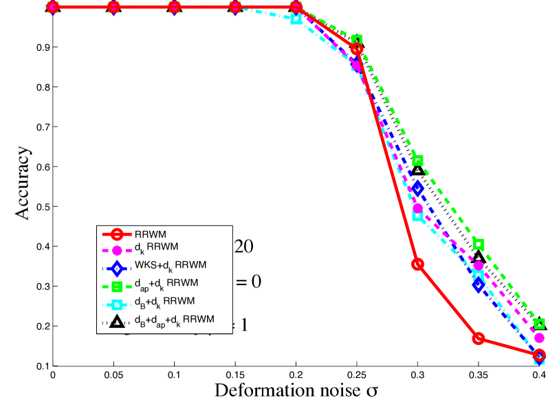
(a)

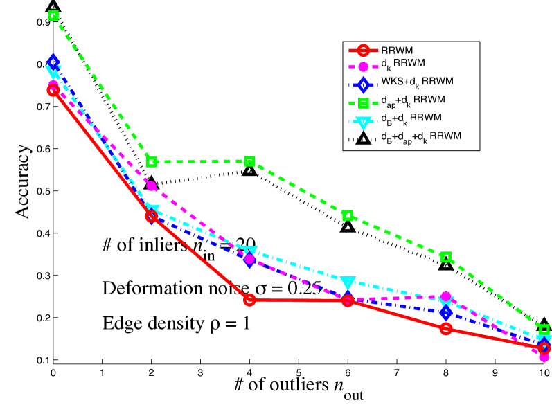
(b)

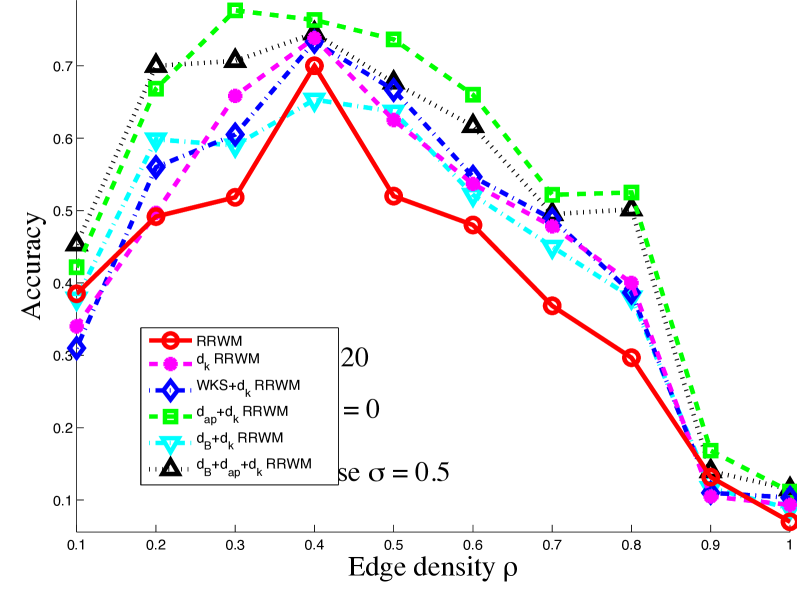
(c)

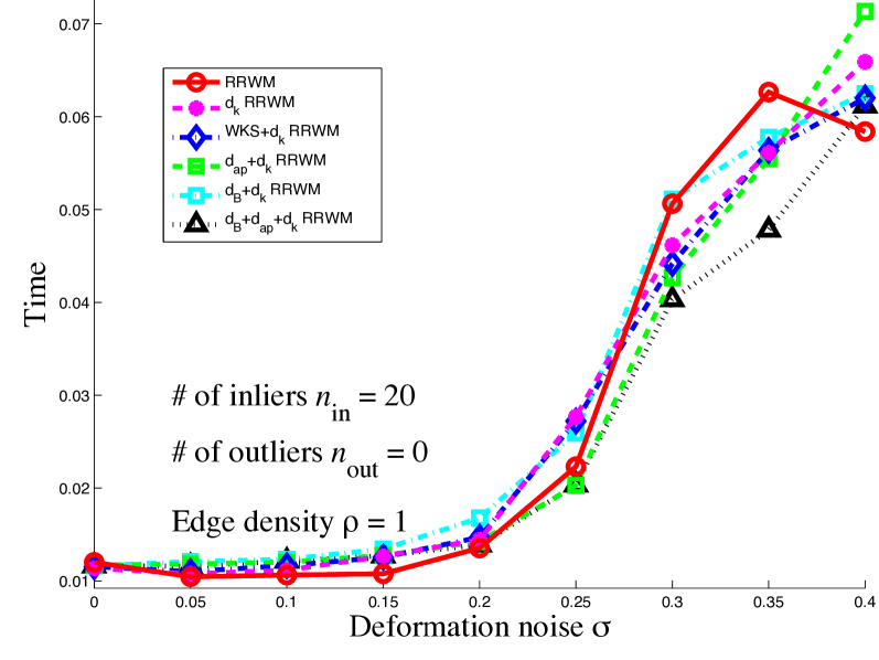
(d)

(e)

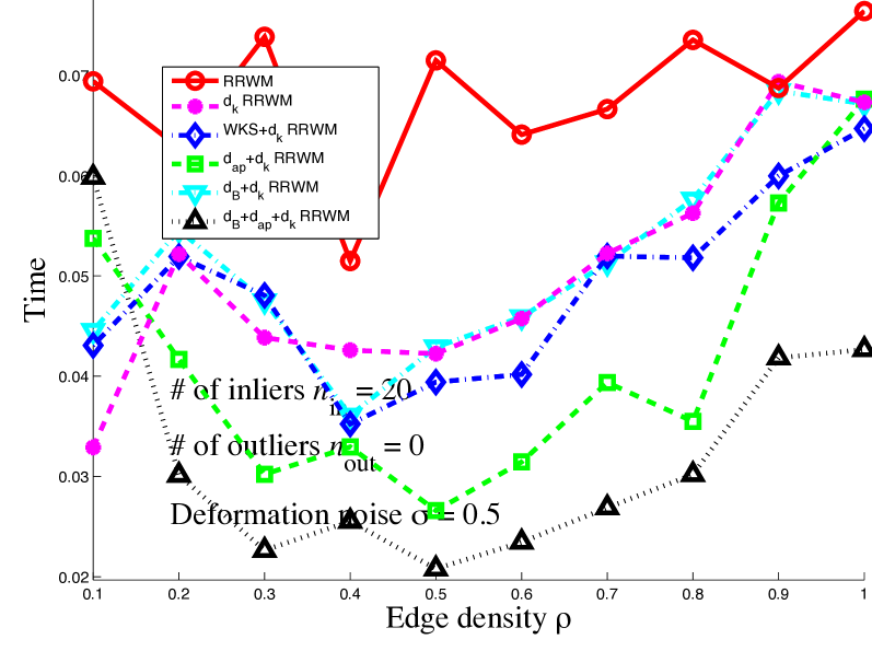
(f)

Figure 1: Matching accuracy and computation time of IQP with different compatibility functions.

In this experiment, we test the matching performance for $W$ constructed using i) only the adjacency matrix [4], ii) only pairwise heat kernel distance $d_{k}(i,j,a,b)$, iii) $d_{k}(i,j,a,b)$ with WKS [11], iv) $d_{k}(i,j,a,b)$ with $d_{\text{ap}}(i,a)$ ($c_{B}=0$,$c_{\text{ap}}=1$), v) $d_{k}(i,j,a,b)$ with $d_{B}(i,a)$ ($c_{B}=1$,$c_{\text{ap}}=0$), and vi) $d_{k}(i,j,a,b)$ with $d_{\text{ap}}(i,a)$ and $d_{B}(i,a)$ ($c_{B}=8$,$c_{\text{ap}}=3$), on three different settings: 1) different levels of deformation noise $\sigma$; 2) different numbers of outliers; 3) different edge densities $\rho$. Fig. 1 shows the average matching accuracy. In the experiment, the number of anchor nodes $|U|=2$. The Red solid curve for RRWM is the baseline approach using the adjacency matrices. From Fig. 1 (a), it can be seen that with the help of learned proximity matrix $B$ and the term $d_{\text{ap}}(i,a)$, the matching results are more robust to noise. In Fig. 1 (c), the matching accuracy is much improved at different edge densities for a relatively large deformation noise ($\sigma=0.5$). Not only the matching accuracy is improved, their corresponding computational time is also decreased as shown in Fig. 1 (f).

5.2 CMU Hotel Sequence

In this experiment, we test our descriptors on the CMU Hotel sequence, which is widely used in performance evaluation of graph matching algorithms as a wide baseline dataset. It consists of 101 frames, and there are 30 feature points labeled consistently across all frames. We build fully connected graphs purely based on the geometry of the feature points, taking the Euclidean distance as the weights between pair of feature points. Affinity matrix $W$ were set up similarly as in Section 5.1. $|U|=2$ nodes were randomly selected as the anchor nodes. We compute the average matching accuracy of each frame to the rest of frames in the sequence. Fig. 2 (a) showed the performance of the matching. As can be seen the matching performance was improved when heat kernel is used in lieu of the adjacency matrix, because the noise tolerance property of the former smoothes out the effect of deformation noise. With the add-on effect of proximity matrix $B$ and $d_{\text{ap}}(i,a)$, furthermore, the matching performance was much improved. Fig. 2 (b,c) showes an example of the matching between the 20th and the 90th frame of the sequence (yellow lines are correct matches and red lines are wrong matches). Matching gives all correct matches, hence is only shown once.

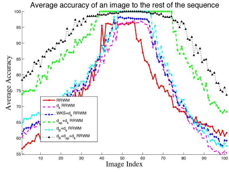
(a) Matching performance

(b) RRWM

(c) $d_{B}+d_{\text{ap}}+d_{k}$ RRWM

Figure 2: Matching on Hotel sequence. Yellow lines depict the correct matches, while red lines show the wrong matches.

In the second part of this experiment, we select to test the influence of the number of anchor nodes on the average matching rate. We intentionally drop off the term $d_{\text{ap}}$ to reduce the side effect, i.e. the matching scheme will be based on $d_{B}+d_{k}$. We increase the number of anchor nodes and compare the matching performance in otherwise the same setting.

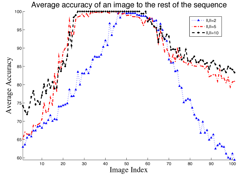
Figure 3: Matching on Hotel sequence with different number of anchor nodes. (Matching scheme is $d_{B}+d_{k}$.)

As shown in Fig. 3, with the increase of the number of anchor nodes, the overall matching performance increased. However, the marginal performance gain seems to have a drop-off with the increase of the number of anchor nodes, since the matching rate gap between $|U|=10$ and $|U|=5$ is much smaller than that between $|U|=5$ and $|U|=2$.

5.3 Pose House Sequence

In this experiment, we test our descriptor on the pose house sequence used in [18]. The dataset consists of 70 frames with 51 labeled feature points across the sequence. The house undergoes large pan and tilt angle change ($0-45^{\circ}$ for pan angle and$0-$$30^{\circ}$ for tilt). The compatibility matrix $W$ is built the same way as in previous experiments. $|U|=2$ nodes were randomly selected as the anchor nodes. Fig. 4 showed the matching results. In Fig. 4 (a), each lump from left to right represent a tilt angle from 0 to $30^{\circ}$ with a $5^{\circ}$ step and within a lump is the pan angle change from left to right for 0 to $45^{\circ}$ with a $5^{\circ}$step. It can been seen that extreme pan angles gave poor results while mid range pan angles yield matches with much higher accuracy — while matching accuracy was not much influenced by the difference in tilt angles. With the addition of our learned proximity matrix $B$, the gap between different pan angles decreases and the overall matching accuracy is superior to others. Fig. 4 (b,c) shows the matching results and the first and last frame of the sequence, which represent the largest pan and tilt angles. Even in this extreme case, it can be seen that our $d_{B}+d_{\text{ap}}+d_{k}$ matching gives useful results, and is much better than the adjacency matrix based matching.

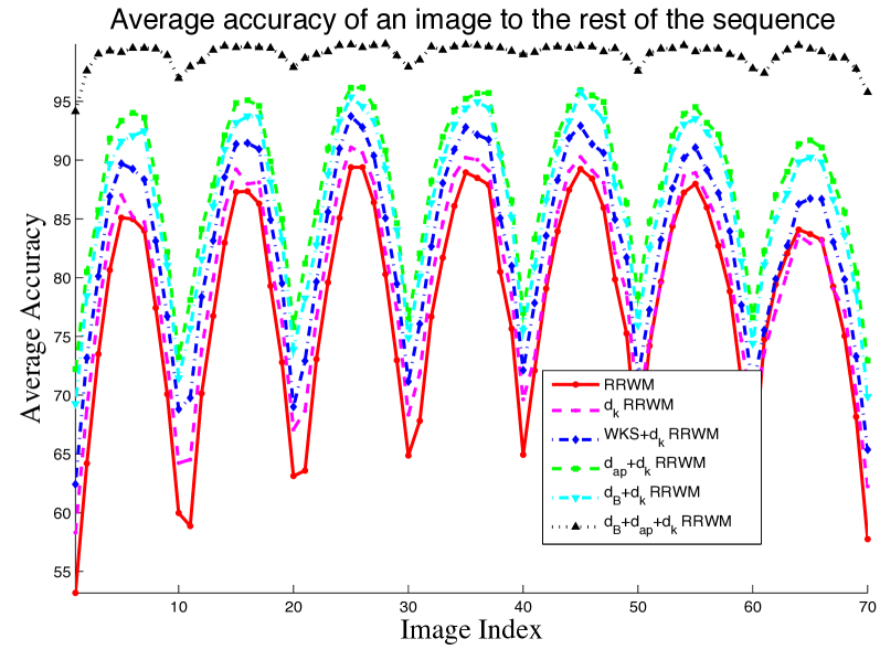
(a) Matching performance

(b) RRWM

(c) $d_{\text{ap}}+d_{k}$ RRWM

(d) $d_{B}+d_{\text{ap}}+d_{k}$ RRWM

Figure 4: Matching on pose house sequence. Yellow lines depict the correct matches, while red lines show the wrong matches.

6 Conclusion

In this paper, we have considered the problem of graph matching where some correspondences are known. We have designed a learning algorithm which uses the anchor correspondences as training samples. The matching problem is set up as an IQP, where we use the learned proximity and heat kernel distance to anchor nodes as first order compatibility, and pairwise heat kernel distance difference as a second order compatibility. With a very small number of anchor nodes ($|U|=2$ in all of the experiments) we have obtained superior performance as compared to the state-of-the-art techniques based on adjacency matrices.

Acknowledgment: The authors would like to acknowledge NSF grants IIS 1016324, CCF 1161480, DMS 1228304, AFOSR FA9550-12-1-0372, the Max Planck Center for Visual Computing and Communications, and a Google research award.

References

- [1] M. Aubry, U. Schlickewei, and D. Cremers. The wave kernel signature: A quantum mechanical approach to shape analysis. In ICCV Workshop 4DMOD, 2011.
- [2] T. Biyikoglu, J. Leydold, and P. F. Stadler. Laplacian eigenvectors of graphs: Perron-Frobenius and Faber-Krahn Type Theorems. Springer, 2007.
- [3] T. Caetano, J. McAuley, C. L., Q. Le, and A. Smola. Learning graph matching. IEEE Trans. PAMI, 31(6):1048–1058, 2009.
- [4] M. Cho, J. Lee, and K. M. Lee. Reweighted random walks for graph matching. In Proceedings of the 11th European conference on Computer vision: Part V, ECCV’10, pages 492–505, Berlin, Heidelberg, 2010. Springer-Verlag.
- [5] T. Cour, P. Srinivasan, and J. Shi. Balanced graph matching. In NIPS’06, pages 313–320, 2006.
- [6] D. Emms, R. C. Wilson, and E. R. Hancock. Graph matching using the interference of continuous-time quantum walks. Pattern Recogn., 42(5):985–1002, May 2009.
- [7] M. Eshera and K. Fu. A graph distance measure for image analysis. IEEE Trans. Syst. Man Cybern., page 398Ð408, 1984.
- [8] S. Gold and A. Rangarajan. A graduated assignment algorithm for graph matching. IEEE Trans. Patt. Anal. Mach. Intell., 18, 1996.
- [9] M. Gori, M. Maggini, and L. Sarti. Exact and approximate graph matching using random walks. IEEE Trans. Pattern Anal. Mach. Intell., 27(7):1100–1111, July 2005.
- [10] D. K. Hammond, P. Vandergheynst, and R. Gribonval. Wavelets on graphs via spectral graph theory. Applied and Computational Harmonic Analysis, 30(2):129–150, Mar. 2011.
- [11] N. Hu and L. Guibas. Spectral Descriptors for Graph Matching. ArXiv e-prints, Apr. 2013. arXiv:1304.1572[cs.CV].
- [12] S. Jouili and S. Tabbone. Graph matching based on node signatures. In Proceedings of GbRPR ’09, pages 154–163, Berlin, Heidelberg, 2009. Springer-Verlag.
- [13] M. Leordeanu and M. Hebert. A spectral technique for correspondence problems using pairwise constraints. In ICCV ’05, pages 1482–1489, Washington, DC, USA, 2005. IEEE Computer Society.
- [14] M. Leordeanu, M. Hebert, and R. Sukthankar. An integer projected fixed point method for graph matching and map inference. In NIPS. Springer, December 2009.
- [15] M. Leordeanu, R. Sukthankar, and M. Hebert. Unsupervised learning for graph matching. Int. J. Comput. Vision, 96(1):28–45, Jan. 2012.
- [16] M. E. Lübbecke and J. Desrosiers. Selected topics in column generation. Oper. Res., 53(6):1007–1023, Nov. 2005.
- [17] B. Luo and E. R. Hancock. Structural graph matching using the em algorithm and singular value decomposition. IEEE Trans. Pattern Anal. Mach. Intell., 23(10):1120–1136, Oct. 2001.
- [18] J. J. McAuley, T. de Campos, and T. S. Caetano. Unified graph matching in euclidean spaces. IEEE Conf. CVPR, pages 1871–1878, 2010.
- [19] H. Qiu and E. R. Hancock. Graph matching and clustering using spectral partitions. Pattern Recogn., 39(1):22–34, Jan. 2006.
- [20] A. Robles-Kelly and E. R. Hancock. String edit distance, random walks and graph matching. In Proceedings of the Joint IAPR International Workshop on Structural, Syntactic, and Statistical Pattern Recognition, pages 104–112, London, UK, UK, 2002. Springer-Verlag.
- [21] A. Robles-Kelly and E. R. Hancock. Graph edit distance from spectral seriation. IEEE Trans. Pattern Anal. Mach. Intell., 27(3):365–378, Mar. 2005.
- [22] C. Schellewald and C. Schnörr. Probabilistic subgraph matching based on convex relaxation. In EMMCVPR’05, pages 171–186, Berlin, Heidelberg, 2005. Springer-Verlag.
- [23] A. Shokoufandeh and S. J. Dickinson. A unified framework for indexing and matching hierarchical shape structures. In IWVF-4, pages 67–84, London, UK, UK, 2001. Springer-Verlag.
- [24] J. Sun, M. Ovsjanikov, and L. Guibas. A concise and provably informative multi-scale signature based on heat diffusion. In Eurographics Symposium on Geometry Processing (SGP), 2009.
- [25] S. Umeyama. An eigendecomposition approach to weighted graph matching problems. IEEE Trans. Pattern Anal. Mach. Intell., 10(5):695–703, 1988.
- [26] B. J. van Wyk and M. A. van Wyk. A pocs-based graph matching algorithm. IEEE Trans. Pattern Anal. Mach. Intell., 26(11):1526–1530, Nov. 2004.
- [27] P. C. Wong, H. Foote, G. Chin, P. Mackey, and K. Perrine. Graph signatures for visual analytics. IEEE trans. on visualization and computer graphics, 12(6):1399–413, 2006.
- [28] E. P. Xing, A. Y. Ng, M. I. Jordan, and S. J. Russell. Distance metric learning with application to clustering with side-information. In NIPS, pages 505–512, 2002.
- [29] M. Zaslavskiy, F. Bach, and J.-P. Vert. A path following algorithm for the graph matching problem. IEEE Transactions on PAMI, 31(12):2227–2242, 2009.
- [30] R. Zass and A. Shashua. Probabilistic graph and hypergraph matching. CVPR, 2008.
- [31] G. Zhao, B. Luo, J. Tang, and J. Ma. Using eigen-decomposition method for weighted graph matching. ICIC’07, pages 1283–1294, 2007.