Finite-time scaling in local bifurcations

Abstract

Finite-size scaling is a key tool in statistical physics, used to infer critical behavior in finite systems. Here we use the analogous concept of finite-time scaling to describe the bifurcation diagram at finite times in discrete dynamical systems. We analytically derive finite-time scaling laws for two ubiquitous transitions given by the transcritical and the saddle-node bifurcation, obtaining exact expressions for the critical exponents and scaling functions. One of the scaling laws, corresponding to the distance of the dynamical variable to the attractor, turns out to be universal. Our work establishes a new connection between thermodynamic phase transitions and bifurcations in low-dimensional dynamical systems, and opens new avenues to identify the nature of dynamical shifts in systems for which only short time series are available.

Introduction

Bifurcations separate qualitatively different dynamics in dynamical systems as one or more parameters are changed. Bifurcations have been mathematically characterized in elastic-plastic materials Nielsen1993 , electronic circuits Kahan1999 , or in open quantum systems Ivanchenko2017 . Also, bifurcations have been theoretically described in population dynamics Rietkerk2004 ; Staver2011 ; Carpenter2011 , in socioecological systems May2008 ; Lade2013 , as well as in fixation of alleles in population genetics and computer virus propagation, to name a few examples Murray2002 ; Ott2002 . More important, bifurcations have been identified experimentally in physical Gil1991 ; Trickey1998 ; Das2007 ; Gomez2017 , chemical Maselko1982 ; Strizhak1996 , and biological systems Dai2012 ; Gu2014 . The simplest cases of local bifurcations, such as the transcritical and the saddle-node bifurcations, only involve changes in the stability and existence of fixed points.

Although, strictly speaking, attractors (such as stable fixed points) are only reached in the infinite-time limit, some studies near local bifurcations have focused on the dependence of the characteristic time needed to approach the attractor as a function of the distance of the bifurcation parameter to the bifurcation point. For example, for the transcritical bifurcation it is known that the transient time, $\tau$, diverges as a power law TEIXEIRA , as $\tau\sim|\mu-\mu_{c}|^{-1}$, with $\mu$ and $\mu_{c}$ being, respectively, the bifurcation parameter and the bifurcation point, while for the saddle-node bifurcation this time goes as $\tau\sim|\mu-\mu_{c}|^{-1/2}$ Strogatz_book (see Trickey1998 for an experimental evidence of this power law in an electronic circuit).

Thermodynamic phase transitions Stanley ; Yeomans1992 , where an order parameter sudden changes its behavior as a response to small changes in one or several control parameters, can be considered as bifurcations. Three important peculiarities of thermodynamic phase transitions within this picture are that the order parameter has to be equal to zero in one of the phases or regimes, that the bifurcation does not arise (in principle) from a simple low-dimensional dynamical system but from the cooperative effects of many-body interactions, and that at thermodynamic equilibrium there is no (macroscopic) dynamics at all. Non-equilibrium phase transitions Marro_Dickman ; Munoz_colloquium are also bifurcations and share these characteristics, except the last one. Particular interest has been paid to second-order phase transitions, where the sudden change of the order parameter is nevertheless continuous and associated to the existence of a critical point.

A key ingredient of second-order phase transitions is finite-size scaling Barber ; Privman , which describes how the sharpness of the transition emerges in the thermodynamic (infinite-system) limit. For instance, if $m$ is magnetization (order parameter), $T$ temperature (control parameter), and $\ell$ system size, for zero applied field and close to the critical point the equation of state can be approximated as a finite-size scaling law,

$$m\simeq\frac{1}{\ell^{\beta/\nu}}g[\ell^{1/\nu}(T-T_{c})],$$ (1)

with $T_{c}$ the critical temperature, $\beta$ and $\nu$ two critical exponents, and $g[y]$ a scaling function fulfilling $g[y]\propto(-y)^{\beta}$ for $y\rightarrow-\infty$ and $g[y]\rightarrow 0$ for $y\rightarrow\infty$.

It has been recently shown that the Galton-Watson branching process (a fundamental stochastic model for the growth and extinction of populations, nuclear reactions, and avalanche phenomena) can be understood as displaying a second-order phase transition Corral_FontClos with finite-size scaling GarciaMillan ; Corral_garciamillan . In a similar spirit, in this article we show how bifurcations in one-dimensional discrete dynamical systems display “finite-time scaling”, analogous to finite-size scaling with time playing the role of system size. We analyze the transcritical and the saddle-node bifurcations for iterated maps and find analytically well-defined scaling functions that generalize the bifurcation diagrams for finite times. The sharpness character of each bifurcation is naturally recovered in the infinite-time limit. As a by-product, we derive the power-law divergence of the characteristic time $\tau$ when $\mu$ is kept constant, off of criticality TEIXEIRA ; Strogatz_book .

I Universal convergence to attractive fixed points

Let us consider a one-dimensional discrete dynamical system, or iterated map, $x_{n+1}=f(x_{n}),$ where $x$ is a real variable, $f(x)$ is a univariate function (which will depend on some non-explicit parameters) and $n$ being discrete time. Let us consider also that the map has an attractive (i.e., stable) fixed point at $x=q$, for which $f(q)=q,$ and that $x_{0}$ belongs to the domain of attraction of the fixed point (more conditions on $x_{0}$ later). It is important to remember that attractiveness in discrete-time systems is characterized by $|f^{\prime}(q)|<1$ (where the prime denotes derivative) Strogatz_book .

We are interested in the behavior of $x_{n}=f^{n}(x_{0})$ for large but finite $n$, where $f^{n}(x_{0})$ denotes the iterated application of the map $n$ times. Naturally, for sufficient large $n$, $f^{n}(x_{0})$ will be close to the attractive fixed point $q$ and we will be able to expand $f(f^{n}(x_{0}))$ around $q$, so,

$$f^{n+1}(x_{0}) = f(f^{n}(x_{0}))=q+M(f^{n}(x_{0})-q)$$ (2)

$$+ C(f^{n}(x_{0})-q)^{2}+\mathcal{O}(q-f^{n}(x_{0}))^{3},$$

with

$$M=f^{\prime}(q)\mbox{ and }C=\frac{f^{\prime\prime}(q)}{2}.$$

Rearranging and introducing the variable $c_{n+1}$, the inverse of the distance to the fixed point at iteration $n+1$, we arrive to

$$c_{n+1}=\frac{1}{q-f^{n+1}(x_{0})}=\frac{c_{n}}{M}+\frac{C}{M^{2}}+\mathcal{O}(q-f^{n}(x_{0}))$$

(we may talk about a distance because, in practice, we calculate the difference in such a way that it is always positive). Iterating this transformation $\ell$ times we get

$$c_{n+\ell}=\frac{c_{n}}{M^{\ell}}+\frac{C(1-M^{\ell})}{M^{\ell+1}(1-M)},$$

to the lowest order GarciaMillan . Introducing the new variable $z=\ell(M-1)$, then, for $\ell$ large one realizes that the second term in the sum grows linearly with $\ell$ and overcomes the first one, and so, $c_{n+\ell}\simeq{C\ell(e^{z}-1)}{e^{-z}}/z.$ Next, considering $\ell$ much larger than $n$, so that $n+\ell\simeq\ell$, we get a scaling law for the dependence of the distance to the attractor on $M$ and $\ell$,

$$q-f^{\ell}(x_{0})=\frac{1}{c_{\ell}}\simeq\frac{1}{C\ell}G(\ell(M-1)),$$ (3)

with scaling function

$$G(z)=\frac{ze^{z}}{e^{z}-1}.$$ (4)

This result has also been obtained in Ref. GarciaMillan for the Galton-Watson model, leading us to realize that this model is governed by a transcritical bifurcation (but restricted to $x_{0}=0$).

The scaling law (3) means that any attractor of a one-dimensional map is approached in the same universal way, as long as a Taylor expansion as the one in Eq. (2) holds, in particular if $f^{\prime\prime}(q)\neq 0$. So we may talk about a “universality class”. The idea is that for different number of iterations $\ell$ one is able to find a value of $M$ (which depends on the parameters of $f(x)$) for which $z=\ell(M-1)$ keeps constant and therefore the rescaled difference with respect the point $M=1$ is constant as well. Note that, in order to have a finite $z$, as $\ell$ is large, $M=f^{\prime}(q)$ will be close to 1, so we will be close to a bifurcation point, corresponding to $M=1$ (where the attractive fixed point will lose its stability). Due to this fact, in the scaling law we can replace $C$ by its value at the bifurcation point $C_{*}$, so, we write $C=C_{*}$ in Eq. (3).

In principle, the value of the initial value $x_{0}$ is not of fundamental importance, we could take for instance $x_{1}=f(x_{0})$ as the initial condition instead, and we would get the same result just replacing $\ell$ by $\ell-1$. For very large $\ell$ this difference plays no role ($\ell\simeq\ell-1$). Therefore, as $\ell$ grows, the influence of the initial condition gets lost, as we can make $\ell$ as large as desired. But on the other hand, $x_{0}$ has to fulfill $x_{0}<q$ if $C_{*}>0$ and $x_{0}>q$ if $C_{*}<0$, in the same way that all the iterations $x_{n}$ (i.e., all the iterations have to be on the same “side” of $q$). The scaling law implies that plotting $[q-f^{\ell}(x_{0})]C_{*}\ell$ versus $\ell(M-1)$ has to yield a data collapse of the curves corresponding to different values of $\ell$ onto the scaling function $G$.

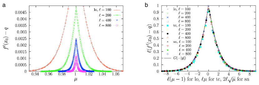
Figure 1: (a) Distance between the $\ell-$th iteration of the logistic map (lo) and its attractor, as a function of the bifurcation parameter $\mu$, for different values of $\ell$. (b) The same data under rescaling (decreasing the density of points, for clarity sake), together with data from the transcritical bifurcation in normal form (tc) and the saddle-node bifurcation (sn). The collapse of the curves into a single one validates the scaling law, Eq. (3), and its universal character. The scaling function is in agreement with $G(-|y|)$. Note that the initial condition $x_{0}$ is taken uniformly randomly between 0.25 and 0.75, which is inside the range necessary for all the iterations to be above the fixed point. This range is, below the bifurcation point, $0<x_{0}<1$ (lo), $0<x_{0}<1+\mu$ (tc), and, above, $1-\mu^{-1}<x_{0}<\mu^{-1}$ (lo), $\mu<x_{0}<1$ (tc), $\sqrt{\mu}<x_{0}<1-\sqrt{\mu}$ (sn).

For example, for the logistic (lo) map Strogatz_book , $f(x)=f_{lo}(x)=\mu x(1-x)$, a transcritical bifurcation takes place at $\mu=1$ and the attractor is at $q=0$ for $\mu\leq 1$ and at $q=1-1/\mu$ for $\mu\geq 1$, which leads to $M_{lo}=f_{lo}^{\prime}(q)=\mu$ for $\mu\leq 1$ and $M_{lo}=2-\mu$ for $\mu\geq 1$, and also to $C_{lo*}=-1$. Therefore, $z=\ell(M-1)=-\ell|\mu-1|$ and $f_{lo}^{\ell}(x_{0})-q\simeq\ell^{-1}G(-\ell|\mu-1|),$ for $x_{0}>q$. Thus, in order to verify the collapse of the curves onto the function $G$, one needs to represent $[f_{lo}^{\ell}(x_{0})-q]\ell$ versus $-\ell|\mu-1|$, or, if one wants to see separately the two regimes, $\mu\gtrless 1$, versus $y=\ell(\mu-1)$. In the latter case the scaling function turns out to be $G(-|y|)$. Figure 1(b) shows precisely this; the nearly perfect data collapse for large $\ell$ is the indication of the fulfillment of the finite-time scaling law. For comparison, Fig. 1(a) shows the same data with no rescaling (i.e., just the distance to the attractor as a function of the bifurcation parameter $\mu$).

If one prefers the normal form of the transcritical (tc) bifurcation (in the discrete case), $f_{tc}(x)=(1+\mu)x-x^{2}$, then the bifurcation takes place at $\mu=0$ (with $q=0$ for $\mu\leq 0$ and $q=\mu$ for $\mu\geq 0$). This leads to exactly the same behavior for $z=-\ell|\mu|$ (or for $y=\ell\mu$ in order to separate the two regimes, as shown overimposed in Fig. 1(b), again with very good agreement).

For the saddle-node (sn) bifurcation (also called fold or tangent bifurcation Kuznetsov_book ), in its normal form (discrete system), $f_{sn}(x)=\mu+x-x^{2}$, the attractor is at $q=\sqrt{\mu}$ (only for $\mu>0$), so the bifurcation is at $\mu=0$, which leads to $M_{sn}=1-2\sqrt{\mu}$ and $C_{sn*}=-1$. The scaling law can be written as

$$f_{sn}^{\ell}(x_{0})-\sqrt{\mu}\simeq\frac{1}{\ell}G(-2\ell\sqrt{\mu}).$$ (5)

To see the data collapse onto the function $G$ one must represent $[f_{sn}^{\ell}(x_{0})-\sqrt{\mu}]\ell$ versus $z=-2\ell\sqrt{\mu}$ (or versus $y=-z$ for clarity sake, as shown also in Fig. 1(b)). If one prefers a horizontal axis linear in $\mu$, one may define $z=-\sqrt{u}$, and then $f_{sn}^{\ell}(x_{0})-\sqrt{\mu}\simeq F(4\ell^{2}\mu)/\ell$, with a transformed scaling function $F(u)=G(-\sqrt{u})={\sqrt{u}}/{(e^{\sqrt{u}}-1)},$ and then use $u=-z^{2}=4\ell^{2}\mu$ for the horizontal axis of the rescaled plot.

Although the key idea of the finite-time scaling law, Eq. (3), is to compare the solution of the system at “corresponding” values of $\ell$ and $\mu$ (such that $z$ is constant, in a sort of law of corresponding states Stanley ), the law can be used as well at fixed $\mu$. At the bifurcation point ($\mu=\mu_{c}$, so $z=0$), we find that the distance to the attractor decays hyperbolically, i.e., $|f^{\ell}(x_{0})-q|=|C_{*}\ell|^{-1}$, as it is well known, see for instance Ref. TEIXEIRA . Out of the bifurcation point, for non-vanishing $\mu-\mu_{c}$ we have $z\rightarrow-\infty$ (as $\ell\rightarrow\infty$) and then $G(z)\rightarrow e^{-z}$, which leads to $f^{\ell}(x_{0})-q\simeq\ell^{-1}e^{-z}\simeq e^{-\ell/\tau}$, where, from the expression for $z$, we find that the characteristic time $\tau$ diverges as $\tau=1/|\mu-\mu_{c}|$ for the transcritical bifurcation (both in normal form and in the logistic form) and as $\tau=1/(2\sqrt{\mu-\mu_{c}})$ for the saddle-node bifurcation (with $\mu_{c}=0$ in the normal form) Trickey1998 . These laws, mentioned in the introduction, have been reported in the literature as scaling laws Strogatz_book , but in order to avoid confusion we suggest to call them power-law divergence laws. Note that this sort of law arises because $G(z)$ is asymptotically exponential; in contrast, the equivalent of $G(z)$ in the equation of state of a magnetic system in the thermodynamic limit is a power law, which leads to the Curie-Weiss law Christensen_Moloney .

II Scaling law for the distance to the fixed point at bifurcation for the iterated value $x_{n}$ in the transcritical bifurcation

In some cases, the distance between $f^{\ell}(x_{0})$ and some constant value of reference will be of more interest than the distance to the attractive fixed point $q$, as the value of $q$ may change with the bifurcation parameter. For the transcritical bifurcation we have two fixed points, $q_{0}$ and $q_{1}$, and they collide and interchange their character (attractive to repulsive, and vice versa) at the bifurcation point. Let us consider that $q_{0}$ is constant independently of the bifurcation parameter (naturally, $q_{1}$ will not be constant), and that “below” the bifurcation point $q_{0}$ is attractive and $q_{1}$ is repulsive, and vice versa “above” the bifurcation. We will be interested in the distance between $q_{0}$ and $f^{\ell}(x_{0})$, i.e., $q_{0}-f^{\ell}(x_{0})$, which, below the bifurcation point corresponds to the quantity calculated previously in Eq. (3), but not above. The reason is that, in there, $q$ was an attractor, but now $q_{0}$ can be attractive or repulsive. Note that, without loss of generality, we can refer $q_{0}-f^{\ell}(x_{0})$ as the distance of $f^{\ell}(x_{0})$ to the “origin”.

Following Ref. GarciaMillan , we need a relation between both fixed points when we are close to the bifurcation point. As, in that case, $q_{1}\simeq q_{0}$, we can expand $f(q_{1})$ around $q_{0}$, to get

$$f(q_{1})=q_{1}=q_{0}+M_{0}(q_{1}-q_{0})+C_{0}(q_{1}-q_{0})^{2}+\mathcal{O}(q_{1}-q_{0})^{3},$$

which leads directly to

$$M_{0}-1=C_{0}(q_{0}-q_{1}),$$ (6)

to the lowest order in $(q_{1}-q_{0})$. Naturally, $M_{0}=f^{\prime}(q_{0})$ and $C_{0}=f^{\prime\prime}(q_{0})/2$. We will also need a relation between $M_{1}=f^{\prime}(q_{1})$ and $M_{0}$. Expanding $f^{\prime}(q_{1})$ around $q_{0}$, $f^{\prime}(q_{1})=M_{1}=M_{0}+2C_{0}(q_{1}-q_{0})+\mathcal{O}(q_{1}-q_{0})^{2},$ which, using Eq. (6), leads to

$$M_{0}-1=1-M_{1},$$ (7)

to the lowest order.

Now let us write $q_{0}-f^{\ell}(x_{0})=q_{0}-q_{1}+q_{1}-f^{\ell}(x_{0})$. For $q_{0}-q_{1}$ we will apply Eq. (6), and for $q_{1}-f^{\ell}(x_{0})$ we can apply Eq. (3), as $q_{1}$ is of attractive nature “above” the bifurcation point; then

$$q_{0}-f^{\ell}(x_{0})\simeq\frac{M_{0}-1}{C_{0}}+\frac{1}{C_{1}\ell}G(\ell(M_{1}-1))$$

(with $C_{1}=f^{\prime\prime}(q_{1})/2$), and defining $y=\ell(M_{0}-1)$ we get (with the form of the scaling function, Eq. (4)),

$$q_{0}-f^{\ell}(x_{0})\simeq\frac{y}{C_{0}\ell}+\frac{1}{C_{1}\ell}\left(\frac{ze^{z}}{e^{z}-1}\right).$$

Using Eq. (7) one realizes that $z=\ell(M_{1}-1)=-\ell(M_{0}-1)=-y$ (so, the $y$ introduced here is the same $y$ introduced above), and therefore,

$$q_{0}-f^{\ell}(x_{0})\simeq\frac{1}{C_{*}\ell}\left(y+\frac{-ye^{-y}}{e^{-y}-1}\right)=\frac{1}{C_{*}\ell}\frac{ye^{y}}{e^{y}-1},$$

where we have used also that $C_{1}=C_{0}=C_{*}$, to the lowest order, with $C_{*}$ the value at the bifurcation point. Therefore, we obtain the same scaling law as in the previous section:

$$q_{0}-f^{\ell}(x_{0})\simeq\frac{1}{C_{*}\ell}G(y),$$ (8)

with the same scaling function $G(y)$ as in Eq. (4), although the rescaled variable $y$ is different here ($y\neq z$, in general). This is possible thanks to the property $y+G(-y)=G(y)$ that the scaling function verifies. Note that the scaling law (1) has the same form as the finite-time scaling (8) and we can identify $\beta=\nu=1$.

Note also that we can identify $M_{0}=f^{\prime}(q_{0})$ with a bifurcation parameter, as it is $M_{0}<1$ “below” the bifurcation point ($M_{0}=1$) and $M_{0}>1$ “above” ($M$ defined in the previous section cannot be a bifurcation parameter as it is never above 1, due to the fact that it is defined with respect the attractive fixed point).

For the transcritical bifurcation of the logistic map we identify $q_{0}=0$ and $M_{0}=\mu$, so $y=\ell(\mu-1)$. For the normal form of the transcritical bifurcation, $q_{0}=0$ but $M_{0}=\mu+1$, so $y=\ell\mu$. Consequently, Fig. 2(a) shows $f^{\ell}(x_{0})$ (the distance to $q_{0}=0$) as a function of $\mu$, for the logistic map and different $\ell$, whereas Fig. 2(b) shows the same results under the corresponding rescaling, together with analogous results for the normal form of the transcritical bifurcation. The data collapse supports the validity of the scaling law (8) with scaling function given by Eq. (4).

III Scaling law for the iterated value $x_{n}$ in the saddle-node bifurcation

Coming back to the saddle-node bifurcation, from Eq. (5) we can isolate the $\ell-$th iterate to get,

$$f^{\ell}(x_{0})\simeq\frac{1}{\ell}\left[\frac{2\ell\sqrt{\mu}}{2}+G(-2\ell\sqrt{\mu})\right]=\frac{1}{\ell}H(y)$$

with $y=-z=2\ell\sqrt{\mu}$ and $H(y)={y(e^{y}+1)}{(e^{y}-1)^{-1}/2}.$ Therefore, the representation of $\ell f^{\ell}(x_{0})$ versus $2\ell\sqrt{\mu}$ unveils the shape of the scaling function $H$. In terms of $u=y^{2}=4\ell^{2}\mu$,

$$f^{\ell}(x_{0})\simeq\frac{1}{\ell}I({u}),\phantom{x}{\rm{with}}\phantom{x}I(u)=H(\sqrt{u})=\frac{\sqrt{u}}{2}\frac{(e^{\sqrt{u}}+1)}{(e^{\sqrt{u}}-1)},$$ (9)

and so, $\ell f^{\ell}(x_{0})$ against $4\ell^{2}\mu$ leads to the collapse of the data onto the scaling function $I(u)$, as shown in Fig. 3. Comparison with the finite-size scaling law (1) allows one to establish $\beta=\nu=1/2$ for this bifurcation (and bifurcation parameter $\mu$, not $\sqrt{\mu}$).

IV Conclusions

By means of scaling laws, we have made clear an analogy between bifurcations and phase transitions, with a direct correspondence between, on the one hand, the bifurcation parameter, the bifurcation point, and the finite-time solution $f^{\ell}(x_{0})$, and, on the other hand, the control parameter, the critical point, and the finite-size order parameter. However, in phase transitions, the sharp change of the order parameter at the critical point arises in the limit of infinite system size; in contrast, in bifurcations, the sharpness at the bifurcation point shows up in the infinite-time limit, $\ell\rightarrow\infty$. So, finite-size scaling in one case corresponds to finite-time scaling in the other.

In addition, we have also been able to derive the power-law divergence of the transient time to reach the attractor off of criticality Trickey1998 ; Strogatz_book ; TEIXEIRA , and also conclude that the results of Ref. GarciaMillan can be directly understood from the transcritical bifurcation underlying the Galton-Watson branching process. Moreover, by using numerical simulations we have tested that the finite-time scaling laws also hold for dynamical systems continuous in time, as well as for the pitchfork bifurcation in discrete time (although with different exponents and scaling function in this case). Let us mention that the use of the finite-time scaling concept by other authors does not correspond with ours. For instance, although Ref. Agoritsas presents a scaling law for finite times, the corresponding exponent $\nu$ there turns to be negative, which is not in agreement with the genuine finite-size scaling around a critical point.

Our results may also allow to identify the nature of bifurcations in systems for which information is limited to short transients, such as in ecological systems. In this way, the scaling relations established in this article could be used as warning signals Scheffer2009 to anticipate the nature of collapses or changes in ecosystems Staver2011 ; Carpenter2011 ; Scheffer2001 ; Scheffer2003 ; Scheffer2009 (due to, e.g., transcritical or saddle-node bifurcations) and in other dynamical suffering dynamical shifts.

Author contributions statement

All authors analysed and discussed the results. All authors reviewed the manuscript.

Additional information

Competing financial interests. The authors declare no competing interests.

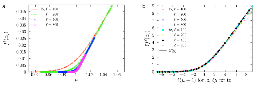
Figure 2: (a) $\ell-$th iteration of the logistic map as a function of the bifurcation parameter $\mu$, for different values of $\ell$. Same initial conditions as in previous figure. (b) Same data under rescaling (decreasing density of points), plus analogous data coming from the transcritical bifurcation in normal form. The data collapse shows the validity of the scaling law, Eq. (8), with scaling function $G(y)$ from Eq. (4).

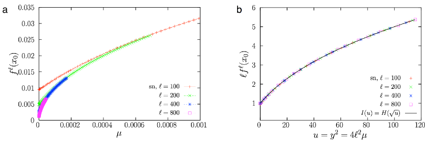
Figure 3: (a) Same as Fig. 2(a) but for the saddle-node bifurcation in normal form. (b) Rescaling of the same data (with decreased density of points). The data collapse supports the scaling law and the scaling function $I(u)$ given by Eq. (9).

References

- [1] M. K. Nielsen and H. L. Schreyer. Bifurcations in elastic-plastic materials. Int. J. of Solids Structures, 30:521–544, 1993.
- [2] S. Kahan and A. C. Sicardi-Schifino. Homoclinic bifurcations in Chua’s circuit. Physica A, 262:144–152, 1999.
- [3] M. Ivanchenko, E. Kozinov, V. Volokitin, A. Liniov, I. Meyerov, and S. Denisov. Classical bifurcation diagrams by quantum means. Annalen der Physik, 529:1600402, 2017.
- [4] M. Rietkerk, S. C. Dekker, P. C. de Ruiter, and J. van de Koppel. Self-organized patchiness and catastrophic shifts in ecosystems. Science, 305:1926–1929, 2004.
- [5] A. C. Staver, S. Archibald, and S. A. Levin. Anticipating critical transitions. Science, 334:230–232, 2011.
- [6] S. R. Carpenter et al. Early warnings of regime shifts: A whole ecosystem experiment. Science, 332:1709–1082, 2011.
- [7] R. M. May and S. A. Levin. Complex systems: Ecology for bankers. Science, 338:344–348, 2008.
- [8] S. J. Lade, A. Tavoni, S. A. Levin, and M. Schlüter. Regime shifts in a socio-ecological system. Theor. Ecol., 6:359–372, 2013.
- [9] J. D. Murray. Mathematical Biology: I. An Introduction. Springer-Verlag, New York, 2002.
- [10] E. Ott. Chaos in Dynamical Systems. Cambridge University Press, Cambridge, 2002.
- [11] L. Gil, G. Balzer, P. Coullet, M. Dubois, and P. Berge. Hopf bifurcation in a broken-parity pattern. Phys. Rev. Lett., 66:3249–3255, 1991.
- [12] S. T. Trickey and L. N. Virgin. Bottlenecking phenomenon near a saddle-node remnant in a Duffing oscillator. Phys. Lett. A, 248:185–190, 1998.
- [13] M. Das, A. Vaziri, A. Kudrolli, and L. Mahadevan. Curvature condensation and bifurcation in an elastic shell. Phys. Rev. Lett., 98:014301, 2007.
- [14] M. Gomez, D. E. Moulton, and D. Vella. Critical slowing down in purely elastic ’snap-through’ instabilities. Nature Phys., 13:142–145, 2017.
- [15] J. Maselko. Determination of bifurcation in chemical systems. An experimental method. Chem. Phys., 67:17–26, 1982.
- [16] P. Strizhak and M. Menzinger. Slow-passage through a supercritical Hopf bifurcation: Time-delayed response in the Belousov-Zhabotinsky reaction in a batch reactor. J. Chem. Phys., 105:10905, 1996.
- [17] L. Dai, D. Vorselen, K. S. Korolev, and J. Gore. Generic indicators of loss of resilience before a tipping point leading to population collapse. Science, 336:1175–1177, 2012.
- [18] H. Gu, B. Pan, G. Chen, and L. Duan. Biological experimental demonstration of bifurcations from bursting to spiking predicted by theoretical models. Nonlinear Dyn., 78:391–407, 2014.
- [19] R. M. N. Teixeira, D. S. Rando, F. C. Geraldo, R. N. C. Filho, J. A. de Oliveira, and E. D. Leonel. Convergence towards asymptotic state in 1-d mappings: A scaling investigation. Phys. Lett. A, 379(18):1246–1250, 2015.
- [20] S. H. Strogatz. Nonlinear Dynamics and Chaos. Perseus Books, Reading, 1994.
- [21] H. E. Stanley. Introduction to Phase Transitions and Critical Phenomena. Oxford University Press, Oxford, 1973.
- [22] J. M. Yeomans. Statistical Mechanics of Phase Transitions. Oxford University Press, New York, 1992.
- [23] J. Marro and R. Dickman. Nonequilibrium Phase Transitions in Lattice Models. Collection Alea-Saclay: Monographs and Texts in Statistical Physics. Cambridge University Press, 1999.
- [24] M. A. Muñoz. Colloquium: Criticality and dynamical scaling in living systems. ArXiv e-prints, 1712:04499, 2017.
- [25] M. N. Barber. Finite-size scaling. In C. Domb and J.L. Lebowitz, editors, Phase Transitions and Critical Phenomena, Vol. 8, pages 145–266. Academic Press, London, 1983.
- [26] V. Privman. Finite-size scaling theory. In V. Privman, editor, Finite Size Scaling and Numerical Simulation of Statistical Systems, pages 1–98. World Scientific, Singapore, 1990.
- [27] A. Corral and F. Font-Clos. Criticality and self-organization in branching processes: application to natural hazards. In M. Aschwanden, editor, Self-Organized Criticality Systems, pages 183–228. Open Academic Press, Berlin, 2013.
- [28] R. Garcia-Millan, F. Font-Clos, and A. Corral. Finite-size scaling of survival probability in branching processes. Phys. Rev. E, 91:042122, 2015.
- [29] A. Corral, R. Garcia-Millan, and F. Font-Clos. Exact derivation of a finite-size scaling law and corrections to scaling in the geometric Galton-Watson process. PLoS ONE, 11(9):e0161586, 2016.
- [30] Y. A. Kuznetsov. Elements of Applied Bifurcation Theory. Springer, New York, 2nd edition, 1998.
- [31] K. Christensen and N. R. Moloney. Complexity and Criticality. Imperial College Press, London, 2005.
- [32] E. Agoritsas, S. Bustingorry, V. Lecomte, G. Schehr, and T. Giamarchi. Finite-temperature and finite-time scaling of the directed polymer free energy with respect to its geometrical fluctuations. Phys. Rev. E, 86:031144, 2012.
- [33] M. G. Scheffer and S. R. Carpenter. Early warning signals for critical transitions. Nature, 461:53–59, 2009.
- [34] M. Scheffer, S. Carpenter, J. A. Foley, C. Folke, and B. Walker. Catastrophic shifts in ecosystems. Nature, 413:591–596, 2001.
- [35] M. G. Scheffer and S. R. Carpenter. Catastrophic regime shifts in ecosystems: linking theory to obervation. Trends Ecol. Evol., 18:648–656, 2003.
Acknowledgements
We have received funding from “La Caixa” Foundation and through the “María de Maeztu” Programme for Units of Excellence in R&D (MDM-2014-0445), as well as from projects FIS2015-71851-P and MTM2014-52209-C2-1-P from the Spanish MINECO, from 2014SGR-1307 (AGAUR), and from the CERCA Programme of the Generalitat de Catalunya.