Measuring the properties of nearly extremal black holes with gravitational waves

Abstract

Characterizing the properties of black holes is one of the most important science objectives for gravitational-wave observations. Astrophysical evidence suggests that black holes that are nearly extremal (i.e. spins near the theoretical upper limit) might exist and, thus, might be among the merging black holes observed with gravitational waves. In this paper, we explore how well current gravitational wave parameter estimation methods can measure the spins of rapidly spinning black holes in binaries. We simulate gravitational-wave signals using numerical-relativity waveforms for nearly-extremal, merging black holes. For simplicity, we confine our attention to binaries with spins parallel or antiparallel with the orbital angular momentum. We find that recovering the holes’ nearly extremal spins is challenging. When the spins are nearly extremal and parallel to each other, the resulting parameter estimates do recover spins that are large, though the recovered spin magnitudes are still significantly smaller than the true spin magnitudes. When the spins are nearly extremal and antiparallel to each other, the resulting parameter estimates recover the small effective spin but incorrectly estimate the individual spins as nearly zero. We study the effect of spin priors and argue that a commonly used prior (uniform in spin magnitude and direction) hinders unbiased recovery of large black-hole spins.

I Introduction

Beginning with the first discovery of gravitational waves (GWs) passing through Earth in 2015, to date the Laser Interferometer Gravitational-Wave Observatory (LIGO) Aasi et al. (2015) and Virgo Acernese et al. (2015) have announced five detections of GWs from merging binary black holes (BBH) Abbott et al. (2016a) (LIGO and Virgo Scientific Collaboration); Abbott et al. (2016b) (LIGO and Virgo Scientific Collaboration); Abbott et al. (2017) (LIGO and Virgo Scientific Collaboration); Abbott et al. (2017a, b). As LIGO and Virgo approach their design sensitivity, they are expected to detect hundreds of merging BH binaries Abadie et al. (2010); Abbott et al. (2017) (LIGO and Virgo Scientific Collaboration).

One important objective of the GW observations is the measurement of the masses and spins of the merging BHs. This is interesting in its own right, but accurate characterization of the systems’ properties is also crucial for astrophysical inference. The masses and the spins of the binary components can reveal information about the way these binaries were formed and about the properties of the BH progenitors. While most formation scenarios predict similar mass distributions for merging BHs Belczynski et al. (2016); Rodriguez et al. (2016a); Stevenson et al. (2017a), it has been suggested that spin measurements might be able to offer information about different formation channels and the BH progenitor properties, e.g. Rodriguez et al. (2016b); Kushnir et al. (2016); Gerosa et al. (2013); Gerosa and Berti (2017); Fishbach et al. (2017); Vitale et al. (2017a); Stevenson et al. (2017b); Talbot and Thrane (2017); Farr et al. (2017a, b); Mandel and O’Shaughnessy (2010); Belczynski et al. (2017).

Besides spin directions, spin magnitudes carry important information as well, since they depend on the angular momentum of the BH’s stellar progenitor and its evolution. At the moment, there remains considerable uncertainty in BH spin measurements, with mild tension between spins inferred from GW observations Abbott et al. (2016a) (LIGO and Virgo Scientific Collaboration); Abbott et al. (2016b) (LIGO and Virgo Scientific Collaboration); Abbott et al. (2017) (LIGO and Virgo Scientific Collaboration); Abbott et al. (2017a, b), stellar evolution models Fuller et al. (2015) and X-ray binary observations Miller and Miller (2014). BH spins inferred from GW observations to date have pointed towards slowly spinning BHs, while inferences of BH spins from X-ray binaries tend to be higher, including some inferred spins that are nearly extremal Gou et al. (2013); McClintock et al. (2006), though these BHs need not be part of the same population Belczynski et al. (2012). By nearly extremal, we mean spins close to the theoretical maximum for a Kerr BH, i.e., dimensionless spins $\chi$ satisfying

$$\chi\equiv\frac{S}{M^{2}}\approx 1,$$ (1)

where $S$ is the spin angular momentum and $M$ is the mass of the spinning BH and throughout the paper we use units where $G=c=1$.

GW observations primarily provide information about the effective spin $\chi_{\rm eff}$, a combination of the spin components along the binary’s orbital angular momentum that is conserved to second post-Newtonian order Racine (2008); Gerosa et al. (2015). Specifically,

$$\chi_{\rm{eff}}=\frac{m_{1}(\vec{\chi}_{1}\cdot\hat{L})+m_{2}(\vec{\chi}_{2}\cdot\hat{L})}{m_{1}+m_{2}},$$ (2)

where $m_{1}$ and $m_{2}$ are the the masses of the larger and smaller BH respectively, $\hat{L}$ is a unit vector in the direction of the orbital angular momentum, and $\vec{\chi}_{1}$ and $\vec{\chi}_{2}$ are the dimensionless spin vectors of the BHs. The apparent discrepancy between GW and X-ray binary measurements has lead to stellar evolution models predicting a bimodality in the spin distribution of BHs. These models suggest that some BHs in future LIGO observations might have large spins that are also aligned with the orbital angular momentum Zaldarriaga et al. (2018); Hotokezaka and Piran (2017).

In this paper we pose the following question: if the BHs in a LIGO source were to have nearly extremal spins, could we tell? To address this question, we simulate GW signals using numerical-relativity (NR) waveforms computed with the Spectral Einstein Code (SpEC) eXtreme Spacetimes (SXS). We use two SpEC simulations from the public Simulating eXtreme Spacetimes (SXS) catalog Mroue et al. (2013); SXS and two new, previously unpublished simulations, including one with the highest BH spins simulated to date. Three simulations have BH spin magnitudes nearly extremal and spin directions either both parallel to $\hat{L}$, both antiparallel to $\hat{L}$ or one spin parallel and one antiparallel. The fourth simulation has moderate BH spins and is included to help assess the impact of large individual spin magnitudes when they point in opposite directions. We then use LIGO parameter estimation methods and tools to infer the properties of the simulated signals, including their masses and spins.

We find that current parameter estimation methods can recover large spins, but only if the effective spin is large (meaning that the spins are either both aligned or both antialigned with the orbital angular momentum) and the signal-to-noise ratio (SNR) is sufficiently high. The recovered spin magnitudes and effective spin are shifted significantly towards less extremal values under the most commonly used spin prior assumption. If, on the other hand, the effective spin is small (meaning that the two BHs’ spins point in opposite directions), we accurately recover the small effective spin but incorrectly recover small individual spins. Our results suggest that if the Universe contains BBH systems with nearly extremal spins, GW inference might fail to tell us.

The rest of this paper is organized as follows. In Sec. II, we describe the NR waveforms, and the simulated GW signals that we generate from them, as well as our parameter estimation methods. In Sec. III, we present our results and discuss the conditions under which we can measure large spins. We conclude in Sec. IV.

II Methods

We calculate our simulated gravitational waveforms using SpEC. SpEC’s methods, including recent improvements enabling more robust simulations of merging BHs with nearly extremal spins, are described in Ref. Scheel et al. (2015) and the references therein.

We consider four numerical gravitational waveforms from merging BHs, each simulated with SpEC. The BHs in each simulation have spins either aligned or antialigned with the orbital angular momentum. Two of these simulations (SXS:BBH:0305 and SXS:BBH:0306) were previously presented in Refs. Abbott et al. (2016a) (LIGO and Virgo Scientific Collaboration); Lovelace et al. (2016); Bohe et al. (2017) and are available in the public SXS catalog SXS , while the other two (SXS:BBH:1124 and SXS:BBH:1137) are new. The configurations are summarized in Table 1: SXS:BBH:1124 has large spins aligned with the orbital angular momentum; SXS:BBH:1137 has large spins antialigned with the orbital angular momentum; SXS:BBH:0306 has two large spin pointing in opposite directions, resulting in a small effective spin; and SXS:BBH:0305 has moderate antiparallel spins and a small effective spin.

SXS:BBH:		$1/q$		$\chi_{1z}$		$\chi_{2z}$		$\chi_{\rm{eff}}$		$N_{\rm orbits}$		$f_{\rm{GW}}$(Hz)
0305		1.22		0.330		-0.439		-0.016		15.2		16.8
0306		1.3		0.961		-0.899		0.152		12.6		19.4
1124		1		0.998		0.998		0.998		25		14.2
1137		1		-0.969		-0.969		-0.969		12		14.9

Table 1: Properties of the SXS simulations used in this paper. The table shows the mass ratio $q$, spin $\chi_{1}$ of the larger BH, spin $\chi_{2}$ of the smaller BH, the resulting $\chi_{\rm{eff}}$, the number of orbits $N_{\rm orbits}$ in the simulation, and the initial GW frequency of the $(\ell=2,m=2)$ mode for a system with a total mass of $70M_{\odot}$.

We use the numerical-relativity (NR) data to simulate GW signals as observed by the two Advanced LIGO detectors with the projected sensitivity for the second observing run Abbott et al. (2013). As is common practice, we do not add detector noise on the simulated signal, which is equivalent to averaging over noise realizations Nissanke et al. (2010). All intrinsic parameters of the simulated signals apart from the total mass are determined by the NR data and are given in Table 1. The total mass of the system is an overall scale factor in vacuum general-relativity that we are free to specify. We select extrinsic parameters such that the orbital angular momentum of the binary points towards the GW detectors and place the binary systems over the Livingston detector, scaling the source distance to achieve a signal-to-noise ratio (SNR) of interest. See Ref. Schmidt et al. (2017) for a description of the details and implementation of the NR injection infrastructure we make use of.

We then analyze the simulated data with the parameter estimation software library LALInference Veitch et al. (2015), which samples the joint multidimensional posterior distribution of the binary parameters. The posterior distribution is calculated through Bayes’ Theorem $p(\vec{x}|d)\sim p(\vec{x})p(d|\vec{x})$, where $p(\vec{x}|d)$ is the joint posterior for the parameters $\vec{x}$ given data $d$, $p(\vec{x})$ is the prior distribution, and $p(d|\vec{x})$ is the likelihood for the data. In GW parameter estimation and under the assumption of stationary and Gaussian detector noise, the likelihood can be expressed as $\text{ln}p(d|\vec{x})\sim-1/2(d-h(\vec{x})|d-h(\vec{x}))$, where parentheses denote the noise-weighted inner product Cutler and Flanagan (1994) evaluated from a lower frequency of 20Hz (24Hz for SXS:BBH:0306) and $h(\vec{x})$ is the model for the GW signal.

The above procedure contains two important ingredients: the prior distribution for the parameters $p(\vec{x})$ and a waveform model for the GW signal $h(\vec{x})$. For the prior, we select a uniform distribution for the sky location and the orientation of the source, a uniform-in-volume distribution for the distance, and a uniform distribution for the component masses. We explore two prior distributions for the spin angular momenta. The first (a ‘uniform $\chi$’ prior) assumes that the spin magnitude and directions have a uniform distribution, $p(\chi)d\chi\propto d\chi$ (this is the default choice for most GW analyses). The second (a ‘volumetric’ prior) assumes that the individual spin components are uniformly distributed, $p(\chi)d\chi\propto\chi^{2}d\chi$. The resulting prior distribution for the effective spin from these two choices is plotted in Fig. 1. Both priors favor small effective spins, though the volumetric prior has more support at high $\chi_{\rm{eff}}$. These prior choices affect parameter inference Vitale et al. (2017b); Gerosa et al. (2017), and we discuss their impact on measuring large spins in Sec. III.

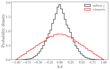
Figure 1: Prior probability density for the effective spin when employing a uniform prior on spin magnitudes and directions (black, ‘uniform $\chi$’), and a uniform prior on spin components (red, ‘volumetric’). In both cases the prior on the component masses is flat.

We employ two waveform models in the LALInference analysis, IMRPhenomPv2 Hannam et al. (2014) and SEOBNRv4 Bohe et al. (2017), which both include the inspiral, merger and ringdown phases of a BBH coalescence. Both models have been extensively used for the analysis of GW signals, see for example Refs. Abbott et al. (2017) (LIGO and Virgo Scientific Collaboration); Abbott et al. (2017a). IMRPhenomPv2 includes the effects of spin-precession in an effective way by parameterizing it through a single effective parameter $\chi_{p}$ Schmidt et al. (2015). SEOBNRv4, on the other hand, assumes that the spins remain aligned with the orbital angular momentum throughout the binary evolution. Both models have been calibrated against nonprecessing NR simulations (including a simulation with both spins at $0.994$ in the case of SEOBNRv4) and have been shown to match well the predictions of NR Bohe et al. (2017). Neither model results in systematic biases in the case of GW150914 Abbott et al. (2017c); Calder n Bustillo et al. (2017). We choose to work with both waveform models both for computational convenience and as an independent cross-check of our results.

III Results

In this section, we present the results of the LALInference parameter estimation study performed on the simulated signals described in Sec. II, and we discuss our ability to robustly characterize nearly extremal BHs in GW observations. Our results indicate that a standard parameter estimation study, such as the one employed by the LIGO and VIRGO collaborations, can lead to a reasonable estimation of the total mass, mass ratio, and effective spin of nearly-extremal BHs. However, we recover a systematic offset in $\chi_{\rm{eff}}$ away from extremality, which is compensated by a systematic bias in the total mass, an outcome of the mass–spin degeneracy. Our parameter estimates are summarized in Table 2 for both priors of Fig. 1.

			Recovered
SXS:BBH:	Parameter	Injected	‘uniform $\chi$’	‘volumetric’
0305	$q$ $M(\textrm{M}_{\odot})$ $\chi_{\text{eff}}$ $\chi_{1z}$ $\chi_{2z}$	0.82 70 -0.016 0.330 -0.439	(0.65,1) ${70.1}^{+2.4}_{-2.3}$ ${-0.013}^{+0.084}_{-0.099}$ ${-0.002}^{+0.271}_{-0.258}$ ${-0.011}^{+0.274}_{-0.386}$	(0.65,1) ${70.0}^{+2.6}_{-2.6}$ ${-0.007}^{+0.086}_{-0.094}$ ${0.158}^{+0.551}_{-0.909}$ ${-0.192}^{+0.989}_{-0.728}$
0306	$q$ $M(\textrm{M}_{\odot})$ $\chi_{\text{eff}}$ $\chi_{1z}$ $\chi_{2z}$	0.77 70 0.152 0.961 -0.899	(0.65,1) ${69.5}^{+3.2}_{-2.9}$ ${0.176}^{+0.100}_{-0.103}$ ${0.201}^{+0.388}_{-0.320}$ ${0.109}^{+0.446}_{-0.411}$	(0.63,1) ${69.5}^{+2.8}_{-2.6}$ ${0.171}^{+0.089}_{-0.088}$ ${0.484}^{+0.427}_{-0.820}$ ${-0.209}^{+1.003}_{-0.701}$
1124	$q$ $M(\textrm{M}_{\odot})$ $\chi_{\text{eff}}$ $\chi_{1z}$ $\chi_{2z}$	1 70 0.998 0.998 0.998	(0.63,1) ${69.4}^{+1.9}_{-1.3}$ ${0.931}^{+0.035}_{-0.046}$ (0.89,1) (0.84,1)	(0.61,1) ${70.8}^{+1.9}_{-1.3}$ ${0.960}^{+0.029}_{-0.055}$ (0.94,1) (0.84,1)
1137	$q$ $M(\textrm{M}_{\odot})$ $\chi_{\text{eff}}$ $\chi_{1z}$ $\chi_{2z}$	1 70 -0.969 -0.969 -0.969	(0.72,1) ${73.8}^{+3.6}_{-2.7}$ ${-0.811}^{+0.150}_{-0.106}$ (-1,-0.65) (-1,-0.59)	(0.77,1) ${74.1}^{+2.9}_{-3.1}$ ${-0.790}^{+0.112}_{-0.144}$ (-1,-0.57) (-1,-0.60)

Table 2: Injected and recovered parameters for the four SXS simulations we study. For each simulated signal (first column) we quote the injected value (third column) and the recovered values (fourth and fifth column) for the mass ratio, the total mass, the effective spin, and the two spin components along the orbital angular momentum (third column). The fourth column shows results obtained with IMRPhenomPv2 and the ‘uniform $\chi$’ prior, while the fifth column presents results with SEOBNRv4 and the ‘volumetric’ prior. The recovered values we quote are either median and 90% credible intervals or one-sided 90% credible intervals, depending on whether the corresponding posterior rails agains a prior boundary, as further explained in, for example, Abbott et al. (2018).

III.1 Source characterization

The effective spin $\chi_{\rm{eff}}$ is one of the best measured spin parameters with GWs. Therefore, it is commonly employed to characterize spin measurability and to study the formation channels of BBHs. Figure 2 shows the marginalized posterior probability density for $\chi_{\rm{eff}}$ for four simulated signals using the NR simulations of Table 1, analyzed with the spin-precessing model IMRPhenomPv2. In all cases, the effective spin posterior is significantly different than the employed ‘uniform $\chi$’ prior (see Fig. 1) indicating that the posteriors are data driven. However, this measurement is not accurate in the case where the true $\chi_{\rm{eff}}$ value is close to the edges of its prior range. Specifically, for cases SXS:BBH:1124 and SXS:BBH:1137, the true value is outside the 99% posterior credible interval, consistent also with the findings of Ref. Afle et al. (2018). In the next section we discuss this bias and its dependence on the specific form of the default, ‘uniform $\chi$’ spin prior employed here, which disfavors large $\chi_{\rm{eff}}$ values.

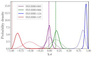
Figure 2: Marginalized posterior probability density for the effective spin for simulated signals at an SNR of $25$ (solid lines) and 12 (dotted lines), and a total mass of $70M_{\odot}$. The data are analyzed with IMRPhenomPv2 and the ‘uniform $\chi$’ prior of Fig. 1 (see Fig. 7 for a reanalysis with the ‘volumetric’ prior). The vertical dashed lines denote the true values of the effective spin. In all cases, the effective spin is measured, though this measurement is biased when the true value of $\chi_{\rm{eff}}$ is close to $\pm 1$. For small values of the true effective spin, the posterior becomes more narrow as the SNR of the signal increases. For large (absolute value) effective spins, on the other hand, the posterior both becomes more narrow and shifts towards the true value as the signal becomes stronger.

Regarding the mass parameters, Fig. 3 shows the two-dimensional posterior for the effective spin and the mass ratio (top panel), and the total mass of the system (bottom panel). It is well known that the effective spin is correlated with either the mass ratio or the total mass, depending on the duration of the signal Cutler and Flanagan (1994). For longer signals that include a long inspiral phase, the effective spin is correlated with the mass ratio, as they both affect the GW phase at the same post-Newtonian order. On the other hand, if a signal consists primarily of the merger phase, the effective spin is correlated with the total mass, since they both affect the frequency of the merger. This trend is visible in Fig. 3, where the $M-\chi_{\rm{eff}}$ correlation is more pronounced than the $q-\chi_{\rm{eff}}$ one for all signals other than SXS:BBH:1124. Since SXS:BBH:1124 has a large positive spin angular momentum it is subject to the effect commonly called “orbital hangup”, an outcome of post-Newtonian spin-orbit coupling Damour (2001); Kidder (1995) (cf. the discussion in Sec. 4.2 of  Scheel et al. (2015) and the references therein). This makes SXS:BBH:1124 last longer and be more inspiral-dominated, and hence more susceptible to the q–$\chi_{\rm{eff}}$ correlation.

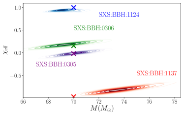
Figure 3: Marginalized two-dimensional posterior probability density for the effective spin parameter and the mass ratio (top panel) and for the effective spin and the total mass (bottom panel) for four simulated signals at an SNR of $25$ and a total mass of $70M_{\odot}$. The data are analyzed with IMRPhenomPv2 and the ‘uniform $\chi$’ prior of Fig. 1. The true value is denoted with a cross of the same color as the corresponding contours. For short signals such as the ones studied here, the effective spin is predominantly correlated with the total mass, as demonstrated in the bottom panel. This correlation is almost broken for the longest duration signal (SXS:BBH:1124, blue posterior) for which the effective spin shows a small correlation with the mass ratio (top panel).

Finally, the properties of the final remnant BH are examined in Fig. 4 which shows the marginalized posterior distribution for the remnant mass and spin. As expected from the discussion of Fig. 3, reliably extracting the properties of the final BH is challenging if the component spins are large. Specifically, the true values are within the 90% posterior credible region only in the SXS:BBH:0305 case.

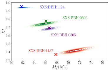
Figure 4: Marginalized two-dimensional posterior probability density for the mass and the spin of the remnant BH for four simulated signals at an SNR of $25$ and a total mass of $70M_{\odot}$. The data are analyzed with IMRPhenomPv2 and the ‘uniform $\chi$’ prior of Fig. 1. The true value is denoted with a cross of the same color as the corresponding contours.

III.2 Spin measurability

In the following we consider the measurability of various spin parameters in more detail. Figure 5 presents posterior probabilities for the binary spin components along the orbital angular momentum (top panel) and $\chi_{\rm{eff}}$ and $\chi_{p}$ (bottom panel). Recall that the spin parameter $\chi_{p}$ quantifies the amount of spin-precession present in the system Schmidt et al. (2015). In each panel, we show results for all four simulated signals at SNR 25; the true parameters are shown as crosses in colors matching the corresponding contours. We find that the large individual spin components can only robustly be measured when both spins are large and parallel to each other. Conversely, configurations with spins antiparallel to each other are recovered as consistent with slowly-spinning binaries, as also alluded to by Fig. 2. The bottom panel of Fig. 5 shows that the $\chi_{p}$ posteriors extend to large values of $\chi_{p}$. However, comparison of these posteriors with the $\chi_{p}$ prior shows that the posterior is prior-dominated and we cannot constrain $\chi_{p}$ from the data Abbott et al. (2016).

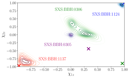
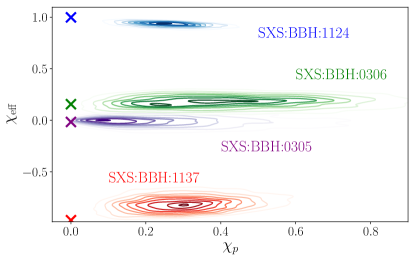
Figure 5: Marginalized two-dimensional posterior probability density for the binary components’ spins along the orbital angular momentum (top panel) and for the effective spin $\chi_{\rm eff}$ and $\chi_{p}$ (bottom panel). The data are analyzed with IMRPhenomPv2 and the uniform prior of Fig. 1. The spin components are not recovered accurately, though the bias is less pronounced when the individual spins are large and both parallel or both antiparallel to the orbital angular momentum.

Figure 6 examines the individual spin magnitudes and shows contours of the two-dimensional posterior probability density for the individual spin magnitudes for the four simulated signals with SNR 25. Crosses indicate the true values for the spins. The recovered individual spins are high when the true spins are nearly extremal and parallel to each other but not when the true spins are antiparallel to each other. This suggests that the individual spin magnitudes of rapidly spinning BHs can only be reliably measured if the spins point in the same direction, creating a larger effective spin $\chi_{\rm eff}$, in agreement with Fig. 5. The difficulty of measuring individual spin magnitudes in general has been previously discussed in Ref. Purrer et al. (2016).

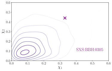
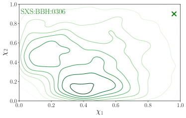
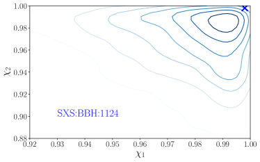
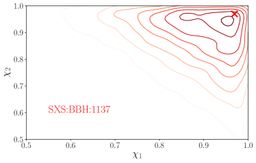
Figure 6: Marginalized two-dimensional posterior probability density for the binary components’ spin magnitudes for four simulated signals with an SNR of $25$ and a total mass of $70M_{\odot}$. Here $\chi_{1}$ and $\chi_{2}$ are the spins of the larger and smaller BH, respectively. The data is analyzed with IMRPhenomPv2 and the uniform prior of Fig. 1. The true value is denoted with a cross symbol. Large individual spins can be measured when the spins are either both parallel or both antiparallel to the orbital angular momentum (1124 and 1137) but not when one spin is parallel and the other antiparallel (0305 and 0306).

III.3 Effect of spin prior

The accuracy of the measurement of the effective spin parameter in Fig. 2 is poor for the two cases where the true value is close to $\pm 1$. In this section, we discuss the effect of the spin prior on the measurement of large spin values Vitale et al. (2017b); Gerosa et al. (2017); Williamson et al. (2017).

Returning to Fig. 2, the dotted lines show the marginalized posteriors for $\chi_{\rm{eff}}$ for signals of SNR 12. Stronger signals enable better parameter measurement and more narrow posterior distributions. This expectation is confirmed for all four systems studied here. Moreover, in the case of SXS:BBH:1124 and SXS:BBH:1137 the posterior not only becomes more narrow, but it also shifts closer to the true value demonstrating the difficulty of measuring large spins.

To explore the effect of prior we employ the ‘volumetric’ prior of Fig. 1, which results in higher prior probability at higher spins, as demonstrated in Fig. 1. Figure 7 shows the posterior distribution for the effective spin for signals analyzed with the spin-aligned waveform model SEOBNRv4 with the ‘uniform $\chi$’ (solid lines) and the ‘volumetric’ (dotted lines) spin prior. In the SXS:BBH:0305 and SXS:BBH:0306 cases, all posteriors are very similar, suggesting that the prior distribution has a lesser effect on the posterior when the effective spin is small.

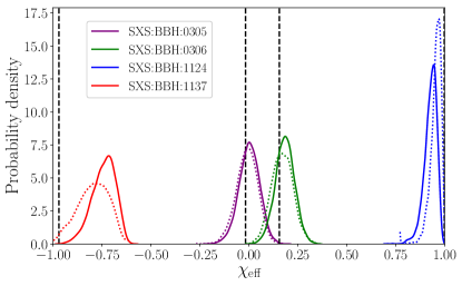
Figure 7: Effective spin posteriors for two choices of the spin prior. Solid lines indicate the ‘uniform $\chi$’ prior and dotted lines denote the ‘volumetric’ prior. This analysis is performed with the spin-sligned waveform model SEOBNRv4.

In the case where $\chi_{\rm{eff}}\sim\pm 1$ on the other hand, the choice of prior has a direct impact on the accuracy of the measurement. Both for SXS:BBH:1124 and SXS:BBH:1137 the ‘volumetric’ prior leads to posteriors that have more support for larger effective spin values, which are now within the 99% posterior credible interval. A similar conclusion can be drawn from Fig. 8, which shows contours for the two-dimensional posterior probability density for the spin components along the orbital angular momentum. As expected, all posteriors derived with the ‘volumetric’ prior have more support for large values of the spin components.

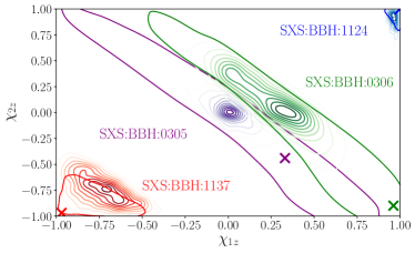
Figure 8: Impact of spin prior on $\chi_{1z}-\chi_{2z}$ recovery with the aligned-spin waveform model SEOBNRv4. Shown are incremental contours for the ‘uniform $\chi$’ prior and a solid-line 90% credible level contour for the ‘volumetric’ prior.

III.4 Effect of signal duration

Due to the finite length of the NR data, all results presented in the above subsections assumed a total mass of $70M_{\odot}$, which is comparable to the total mass of GW150914 Abbott et al. (2016a) (LIGO and Virgo Scientific Collaboration). If the total mass of the system is lower than this value, the start of the numerical waveform falls within the sensitive frequencies of the detector, potentially affecting the results of parameter estimation Mandel et al. (2014). To study the effect of the signal duration on our results, instead, we use the waveform model IMRPhenomPv2 to simulate the GW data with parameters equal to those of SXS:BBH:1124 and SXS:BBH:1137 but with a total mass of $30,50,$ and $70M_{\odot}$. We employ the same model for signal recovery and find that the resulting posteriors are very similar, suggesting that our main conclusions are unaffected by the signal duration.

III.5 Model accuracy

Our study suggests that current analyses are sub-optimal for characterizing signals with large spins. However, the waveform models used for these analyses may also lose accuracy at this challenging region of the parameter space Bohe et al. (2017). This prompts the question: is it hard to measure large spins because of the posterior properties or because the waveform models employed misbehave? In order to fully address this question we would have to perform parameter estimation directly using NR waveforms, something that is currently impossible for the region of the parameter space we are interested in. However, below we discuss evidence suggesting that the difficulty to measure large spins has less to do with the accuracy of the models, and more with the properties of the likelihood function and the prior choices.

First, when the SNR of the signal is increased, the posterior distribution for $\chi_{\rm{eff}}$ in the SXS:BBH:1137 and SXS:BBH:1124 cases shifts towards the true value, as shown in Fig. 2. Since systematic errors caused by model inaccuracies do not depend on the SNR, the shift in the posterior suggests it is mainly the prior that keeps the posteriors away from large $\chi_{\rm{eff}}$ values.

Second, we repeat the analysis described above and compute the posterior for the effective spin parameter using a simulated signal created with the numerical waveforms and with the IMRPhenomPv2 waveform model. We find a large similarity between the posterior obtained with the different data, as shown in Fig. 9. Specifically, the shift in the posterior due to the change of data in Fig. 9 is smaller than the shift due to changing the spin prior in Fig. 7. This suggests that at the injected parameter values the NR waveform and the data created with IMRPhenomPv2 do not possess noticeable differences as far as parameter estimation is concerned.

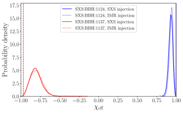
Figure 9: Similar to Fig. 2 for signals created with NR data (solid lines), and with the IMRPhenomPv2 waveform model (dotted lines). The similarity between the solid and the dotted curves suggest that systematic difference between NR and waveform models are not the dominant cause of our conclusion that large spins are difficult to measure.

Third, we employ a figure of merit commonly used in waveform modeling, namely the overlap between the signal and the template, defined as $(d|h(\vec{x}))/\sqrt{(d|d)(h(\vec{x})|h(\vec{x}))}$. Figure 10 shows a scatter plot of the posterior samples for the SXS:BBH:1137 case of the lower panel of Fig. 3. The samples are colored by their overlap value; we find overlaps around $99.5\%$ in the region of the injected parameters, and they drop as we move away from the true parameters. We obtain similar results for the other three NR signals studied here and the SEOBNRv4 model. The high value of overlap further suggests that systematic biases are subdominant for this region of the parameter space and for this SNR value Chatziioannou et al. (2017).

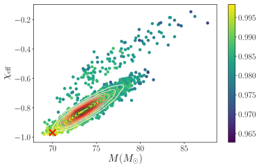
Figure 10: Similar to the bottom panel of Fig. 3 for the case of SXS:BBH:1137 with 5000 scattered posterior samples colored by the value of their overlap with the simulated data. The overlap achieved close to the injected value is in the 99.5% range.

IV Conclusions

In this paper, we assess the prospects of extracting the spins of nearly extremal BHs in binaries with GW measurements. We find that measurement of large spins is challenging. Favorable conditions occur when both spins are large and parallel to each other, but even in this case our posteriors are biased away from extremal effective spins. We argue that this is due to the commonly used spin priors that disfavor large spins.

Additionally, extremal spins are close to the edge of the spin priors. This situation is similar to the case of measuring the mass ratio (or the symmetric mass ratio) of equal-mass systems. In fact, when the posterior distribution of a parameter rails agains a prior edge, it is customary to use one-sided credible intervals or highest-probability-density intervals (for an extended discussion, see Abbott et al. (2018)). However, we find this is not the case for the effective spin, since its posterior typically does not rail against the prior edge (see Fig. 2). We attribute this to the spin prior, which drops to vanishingly small values as $\chi_{\rm eff}\to\pm 1$. In order to overcome this trend and obtain a likelihood-dominated effective spin posterior, a signal with large SNR is needed.

Our results showcase again the importance of priors and prior bounds in GW inference and suggest the use of a wide range of spin priors. This will not only allow us to study physical effects such as the large spins described here, but can also enable further studies such as the hierarchical analysis described in Farr et al. (2017a).

V Acknowledgments

We are pleased to thank Sebastian Khan and Jacob Lange for useful discussions on producing simulated GW signals with NR data. We would also like to thank Joshua Smith and Jocelyn Read for helpful discussions and Leo Stein and Juan Calderon Bustillo for comments on the manuscript. This work was supported in part by National Science Foundation grants PHY-1606522 and PHY-1654359 to Cal State Fullerton. We gratefully acknowledge support for this research at Caltech from NSF grants PHY-1404569, PHY-1708212, and PHY-1708213 and the Sherman Fairchild Foundation and at Cornell from NSF Grant PHY-1606654 and the Sherman Fairchild Foundation.

References

- Aasi et al. (2015) J. Aasi et al. (LIGO Scientific), Class. Quant. Grav. 32, 074001 (2015), arXiv:1411.4547 [gr-qc] .
- Acernese et al. (2015) F. Acernese et al. (VIRGO), Class. Quant. Grav. 32, 024001 (2015), arXiv:1408.3978 [gr-qc] .
- Abbott et al. (2016a) (LIGO and Virgo Scientific Collaboration) B. P. Abbott et al. (LIGO and Virgo Scientific Collaboration), Phys. Rev. Lett. 116, 061102 (2016a), arXiv:1602.03837 [gr-qc] .
- Abbott et al. (2016b) (LIGO and Virgo Scientific Collaboration) B. P. Abbott et al. (LIGO and Virgo Scientific Collaboration), Phys. Rev. Lett. 116, 241103 (2016b), arXiv:1606.04855 [gr-qc] .
- Abbott et al. (2017) (LIGO and Virgo Scientific Collaboration) B. P. Abbott et al. (LIGO and Virgo Scientific Collaboration), Phys. Rev. Lett. 118, 221101 (2017), arXiv:1706.01812 [gr-qc] .
- Abbott et al. (2017a) B. P. Abbott et al. (Virgo, LIGO Scientific), Phys. Rev. Lett. 119, 141101 (2017a), arXiv:1709.09660 [gr-qc] .
- Abbott et al. (2017b) B. P. Abbott et al. (Virgo, LIGO Scientific), Astrophys. J. 851, L35 (2017b), arXiv:1711.05578 [astro-ph.HE] .
- Abadie et al. (2010) J. Abadie, B. P. Abbott, R. Abbott, M. Abernathy, T. Accadia, F. Acernese, C. Adams, R. Adhikari, P. Ajith, B. Allen, and et al., Classical and Quantum Gravity 27, 173001 (2010), arXiv:1003.2480 [astro-ph.HE] .
- Belczynski et al. (2016) K. Belczynski, D. E. Holz, T. Bulik, and R. O’Shaughnessy, Nature 534, 512 (2016), arXiv:1602.04531 [astro-ph.HE] .
- Rodriguez et al. (2016a) C. L. Rodriguez, C.-J. Haster, S. Chatterjee, V. Kalogera, and F. A. Rasio, Astrophys. J. 824, L8 (2016a), arXiv:1604.04254 [astro-ph.HE] .
- Stevenson et al. (2017a) S. Stevenson, A. Vigna-G mez, I. Mandel, J. W. Barrett, C. J. Neijssel, D. Perkins, and S. E. de Mink, (2017a), 10.1038/ncomms14906, [Nature Commun.8,14906(2017)], arXiv:1704.01352 [astro-ph.HE] .
- Rodriguez et al. (2016b) C. L. Rodriguez, M. Zevin, C. Pankow, V. Kalogera, and F. A. Rasio, Astrophys. J. 832, L2 (2016b), arXiv:1609.05916 [astro-ph.HE] .
- Kushnir et al. (2016) D. Kushnir, M. Zaldarriaga, J. A. Kollmeier, and R. Waldman, Mon. Not. Roy. Astron. Soc. 462, 844 (2016), arXiv:1605.03839 [astro-ph.HE] .
- Gerosa et al. (2013) D. Gerosa, M. Kesden, E. Berti, R. O’Shaughnessy, and U. Sperhake, Phys. Rev. D87, 104028 (2013), arXiv:1302.4442 [gr-qc] .
- Gerosa and Berti (2017) D. Gerosa and E. Berti, Phys. Rev. D95, 124046 (2017), arXiv:1703.06223 [gr-qc] .
- Fishbach et al. (2017) M. Fishbach, D. E. Holz, and B. Farr, Astrophys. J. 840, L24 (2017), arXiv:1703.06869 [astro-ph.HE] .
- Vitale et al. (2017a) S. Vitale, R. Lynch, R. Sturani, and P. Graff, Class. Quant. Grav. 34, 03LT01 (2017a), arXiv:1503.04307 [gr-qc] .
- Stevenson et al. (2017b) S. Stevenson, C. P. L. Berry, and I. Mandel, Mon. Not. Roy. Astron. Soc. 471, 2801 (2017b), arXiv:1703.06873 [astro-ph.HE] .
- Talbot and Thrane (2017) C. Talbot and E. Thrane, Phys. Rev. D96, 023012 (2017), arXiv:1704.08370 [astro-ph.HE] .
- Farr et al. (2017a) W. M. Farr, S. Stevenson, M. Coleman Miller, I. Mandel, B. Farr, and A. Vecchio, Nature 548, 426 (2017a), arXiv:1706.01385 [astro-ph.HE] .
- Farr et al. (2017b) B. Farr, D. E. Holz, and W. M. Farr, (2017b), arXiv:1709.07896 [astro-ph.HE] .
- Mandel and O’Shaughnessy (2010) I. Mandel and R. O’Shaughnessy, Numerical relativity and data analysis. Proceedings, 3rd Annual Meeting, NRDA 2009, Potsdam, Germany, July 6-9, 2009, Class. Quant. Grav. 27, 114007 (2010), arXiv:0912.1074 [astro-ph.HE] .
- Belczynski et al. (2017) K. Belczynski et al., (2017), arXiv:1706.07053 [astro-ph.HE] .
- Fuller et al. (2015) J. Fuller, M. Cantiello, D. Lecoanet, and E. Quataert, Astrophys. J. 810, 101 (2015), arXiv:1502.07779 [astro-ph.SR] .
- Miller and Miller (2014) M. C. Miller and J. M. Miller, Phys. Rept. 548, 1 (2014), arXiv:1408.4145 [astro-ph.HE] .
- Gou et al. (2013) L. Gou, J. E. McClintock, R. A. Remillard, J. F. Steiner, M. J. Reid, et al., (2013), arXiv:1308.4760 [astro-ph.HE] .
- McClintock et al. (2006) J. E. McClintock, R. Shafee, R. Narayan, R. A. Remillard, S. W. Davis, et al., Astrophys.J. 652, 518 (2006), arXiv:astro-ph/0606076 [astro-ph] .
- Belczynski et al. (2012) K. Belczynski, T. Bulik, and C. L. Fryer, ArXiv e-prints (2012), arXiv:1208.2422 [astro-ph.HE] .
- Racine (2008) E. Racine, Phys. Rev. D78, 044021 (2008), arXiv:0803.1820 [gr-qc] .
- Gerosa et al. (2015) D. Gerosa, M. Kesden, U. Sperhake, E. Berti, and R. O’Shaughnessy, Phys. Rev. D92, 064016 (2015), arXiv:1506.03492 [gr-qc] .
- Zaldarriaga et al. (2018) M. Zaldarriaga, D. Kushnir, and J. A. Kollmeier, Mon. Not. Roy. Astron. Soc. 473, 4174 (2018), arXiv:1702.00885 [astro-ph.HE] .
- Hotokezaka and Piran (2017) K. Hotokezaka and T. Piran, Astrophys. J. 842, 111 (2017), arXiv:1702.03952 [astro-ph.HE] .
- eXtreme Spacetimes (SXS) S. eXtreme Spacetimes (SXS) Collaboration, http://black-holes.org/SpEC.html.
- Mroue et al. (2013) A. H. Mroue, M. A. Scheel, B. Szilágyi, H. P. Pfeiffer, M. Boyle, D. A. Hemberger, L. E. Kidder, G. Lovelace, S. Ossokine, N. W. Taylor, A. Zenginoglu, L. T. Buchman, T. Chu, E. Foley, M. Giesler, R. Owen, and S. A. Teukolsky, Phys. Rev. Lett. 111, 241104 (2013), arXiv:1304.6077 [gr-qc] .
- (35) http://www.black-holes.org/waveforms.
- Scheel et al. (2015) M. A. Scheel, M. Giesler, D. A. Hemberger, G. Lovelace, K. Kuper, M. Boyle, B. Szilágyi, and L. E. Kidder, Class. Quant. Grav. 32, 105009 (2015), arXiv:1412.1803 [gr-qc] .
- Lovelace et al. (2016) G. Lovelace et al., Class. Quant. Grav. 33, 244002 (2016), arXiv:1607.05377 [gr-qc] .
- Bohe et al. (2017) A. Bohe et al., Phys. Rev. D95, 044028 (2017), arXiv:1611.03703 [gr-qc] .
- Abbott et al. (2013) B. P. Abbott et al. (VIRGO, LIGO Scientific), (2013), 10.1007/lrr-2016-1, [Living Rev. Rel.19,1(2016)], arXiv:1304.0670 [gr-qc] .
- Nissanke et al. (2010) S. Nissanke, D. E. Holz, S. A. Hughes, N. Dalal, and J. L. Sievers, Astrophys. J. 725, 496 (2010), arXiv:0904.1017 [astro-ph.CO] .
- Chatziioannou et al. (2014) K. Chatziioannou, N. Cornish, A. Klein, and N. Yunes, Phys. Rev. D89, 104023 (2014), arXiv:1404.3180 [gr-qc] .
- Chatziioannou et al. (2015) K. Chatziioannou, N. Cornish, A. Klein, and N. Yunes, Astrophys. J. 798, L17 (2015), arXiv:1402.3581 [gr-qc] .
- Farr et al. (2016) B. Farr et al., Astrophys. J. 825, 116 (2016), arXiv:1508.05336 [astro-ph.HE] .
- Schmidt et al. (2017) P. Schmidt, I. W. Harry, and H. P. Pfeiffer, (2017), arXiv:1703.01076 [gr-qc] .
- Veitch et al. (2015) J. Veitch et al., Phys. Rev. D91, 042003 (2015), arXiv:1409.7215 [gr-qc] .
- Cutler and Flanagan (1994) C. Cutler and E. E. Flanagan, Phys. Rev. D 49, 2658 (1994).
- Vitale et al. (2017b) S. Vitale, D. Gerosa, C.-J. Haster, K. Chatziioannou, and A. Zimmerman, Phys. Rev. Lett. 119, 251103 (2017b), arXiv:1707.04637 [gr-qc] .
- Gerosa et al. (2017) D. Gerosa, S. Vitale, C.-J. Haster, K. Chatziioannou, and A. Zimmerman, in IAU Symposium 338: Gravitational Wave Astrophysics: Early Results from GW Searches and Electromagnetic Counterparts Baton Rouge, LA, USA, October 16-19, 2017 (2017) arXiv:1712.06635 [astro-ph.HE] .
- Hannam et al. (2014) M. Hannam, P. Schmidt, A. Boh , L. Haegel, S. Husa, F. Ohme, G. Pratten, and M. P rrer, Phys. Rev. Lett. 113, 151101 (2014), arXiv:1308.3271 [gr-qc] .
- Schmidt et al. (2015) P. Schmidt, F. Ohme, and M. Hannam, Phys. Rev. D91, 024043 (2015), arXiv:1408.1810 [gr-qc] .
- Abbott et al. (2017c) B. P. Abbott et al. (Virgo, LIGO Scientific), Class. Quant. Grav. 34, 104002 (2017c), arXiv:1611.07531 [gr-qc] .
- Calder n Bustillo et al. (2017) J. Calder n Bustillo, P. Laguna, and D. Shoemaker, Phys. Rev. D95, 104038 (2017), arXiv:1612.02340 [gr-qc] .
- Abbott et al. (2018) B. P. Abbott et al. (Virgo, LIGO Scientific), (2018), arXiv:1805.11579 [gr-qc] .
- Afle et al. (2018) C. Afle et al., (2018), arXiv:1803.07695 [gr-qc] .
- Damour (2001) T. Damour, Phys. Rev. D 64, 124013 (2001), arXiv:gr-qc/0103018 [gr-qc] .
- Kidder (1995) L. E. Kidder, Phys. Rev. D52, 821 (1995), arXiv:gr-qc/9506022 .
- Abbott et al. (2016) B. P. Abbott et al. (Virgo, LIGO Scientific), Phys. Rev. Lett. 116, 241102 (2016), arXiv:1602.03840 [gr-qc] .
- Purrer et al. (2016) M. Purrer, M. Hannam, and F. Ohme, Phys. Rev. D93, 084042 (2016), arXiv:1512.04955 [gr-qc] .
- Williamson et al. (2017) A. R. Williamson, J. Lange, R. O’Shaughnessy, J. A. Clark, P. Kumar, J. Calder n Bustillo, and J. Veitch, Phys. Rev. D96, 124041 (2017), arXiv:1709.03095 [gr-qc] .
- Mandel et al. (2014) I. Mandel, C. P. Berry, F. Ohme, S. Fairhurst, and W. M. Farr, Class.Quant.Grav. 31, 155005 (2014), arXiv:1404.2382 [gr-qc] .
- Chatziioannou et al. (2017) K. Chatziioannou, A. Klein, N. Yunes, and N. Cornish, Phys. Rev. D95, 104004 (2017), arXiv:1703.03967 [gr-qc] .