Moment Inequalities in the Context of Simulated and Predicted Variables

Abstract

This paper explores the effects of simulated moments on the performance of inference methods based on moment inequalities. Commonly used confidence sets for parameters are level sets of criterion functions whose boundary points may depend on sample moments in an irregular manner. Due to this feature, simulation errors can affect the performance of inference in non-standard ways. In particular, a (first-order) bias due to the simulation errors may remain in the estimated boundary of the confidence set. We demonstrate, through Monte Carlo experiments, that simulation errors can significantly reduce the coverage probabilities of confidence sets in small samples. The size distortion is particularly severe when the number of inequality restrictions is large. These results highlight the danger of ignoring the sampling variations due to the simulation errors in moment inequality models. Similar issues arise when using predicted variables in moment inequalities models. We propose a method for properly correcting for these variations based on regularizing the intersection of moments in parameter space, and we show that our proposed method performs well theoretically and in practice.

Keywords: Simulated moments, Moment inequalities, Smoothable convex functions

1 Introduction

Recently, estimating with moment inequalities rather than traditional equalities has proven increasingly popular (Tamer, 2010). Even in contexts when a model is difficult or even impossible to compute exactly, economic theory may provide inequalities that are amenable to estimation. Thus, many of the examples in which moment inequalities are attractive are also examples in which computing the model is complex. This model complexity also leads the author to use simulation techniques, often to address the calculation of integrals over complex objects. However, the role of simulation in moment inequality estimation has been largely unexplored.

In this paper, we argue that using simulation or predicted values in the context of moment inequalities has important implications both for determining identified sets and for inference. We show that simulated moment inequality estimators suffer from small sample bias, which is a result of the irregular nature of the estimator. This irregularity is introduced by the following mechanism. Rather than finding optimal parameters through some kind of extremum estimator, moment inequality estimators typically build the estimated identified set or confidence region through level set computations, such as in Chernozhukov et al. (2007) and Andrews & Barwick (2012). The level set is defined by the intersection of moments, and at these intersections, the objective function may depend on the underlying moments in an irregular way. That is, at such intersections, the distribution of the objective function can be particularly sensitive to perturbations to the underlying moments. Since these intersections often define the maximum or minimum of the confidence interval in a particular direction, they determine the range of parameters in the confidence interval, and thus the intersections are often of greatest interest. Whereas approximation error (for instance, due to simulation) in moment equality estimators for small samples is of second order importance, we show that irregular objective functions promote approximation error in small samples to first order importance.

In this paper, we first describe formally the phenomena that we are interested in. A starting place is the well-known result for moment equalities that estimation that requires simulation is consistent, even for a fixed number of draws (McFadden, 1989; Pakes & Pollard, 1989). Moment inequality estimators are similar to moment equalities because they take means over simulated or predicted variables before transforming them into an objective function. Simulated moment functions are consistent (and asymptotically unbiased) for their population counterparts $E[m(X,\cdot)]$ for a finite number of draws. This ensures that level-set estimators of identified sets (Chernozhukov et al., 2007) are also consistent in the Hausdorff distance.

We show that the similarity breaks down when it comes to inference in finite samples, due to the irregular feature of the objective function. We explore this phenomenon in two Monte Carlo experiments. The first one focuses on estimation of the point of intersection of multiple simulated moment inequalities, and is meant to maximize the scope of the problem we discuss. The second is a more realistic treatment: We study an entry game in the spirit of Ciliberto & Tamer (2009). Moment inequalities are generated by the lower and upper bounds of entry probabilities conditional on covariates that are classified into a finite number of bins. In our Monte Carlo experiments, we find that the coverage probabilities of the confidence regions are distorted severely when there are bins with a limited number of observations and a small number of simulation draws is used. The presence of such bins is common in empirical applications. Therefore, inference methods that properly account for the effects of simulation are needed.

We propose a new solution to the problems associated with the irregularity of the objective function, including those due to simulated moments. The key is that the commonly used objective functions involve smoothable convex functions (Beck & Teboulle, 2012). Our method “regularizes” or smoothes the objective function, and we show that this method leads to a straightforward bias correction method. While the idea of regularization appears in some other contexts, such as Haile & Tamer (2003), Chernozhukov et al. (2015) and Masten & Poirier (2017), we formally show that this approach has uniform validity in the context of inference with simulated variables. Our regularization method is based on the class of $\mu$-smooth approximations studied in the non-smooth optimization literature (Nesterov, 2005; Beck & Teboulle, 2012). We provide conditions on the choice of approximating functions and regularization parameters that ensure the uniform validity of an inference procedure that combines the proposed regularization scheme with a straightforward bootstrap resampling. In addition to being attractive theoretically, we show that this approach performs well in practice, even relative to techniques that implement bias correction via the adjustment of the critical value such as Andrews & Soares (2010) and Chernozhukov et al. (2013). Specifically, our Monte Carlo experiments show that the proposed method controls the size well and is often less conservative than the existing methods.

Before moving on, we want to stress that simulation is common in many well-known applications of moment inequalities. For instance, Haile & Tamer (2003) simulate bids in order to place bounds on the value of participants in an auction. Ciliberto & Tamer (2009) simulate an entry game to determine upper and lower bounds for the probability of a firm entering under different equilibrium selection mechanisms. Ho (2009) uses inequalities to study network formation between hospitals and insurers, and uses predicted profit from a network as an explanatory variable for the firm’s choices. The profit function is based on a random coefficient logit demand function as in Berry et al. (1995), which involves simulation. Eizenberg (2013) studies firms choosing product characteristics, and also relies on simulated demand predictions drawn from a Berry et al. (1995) demand system. Kawai & Watanabe (2013) simulates market effects in a model of strategic voting that uses moment inequalities to address unobserved beliefs about other voters. Although not strictly moment inequalities, the method of Bajari et al. (2007) uses simulation in the context of a minimum distance estimator based on inequalities to study dynamic oligopoly games. Well-known applications are Ryan (2012) and Fowlie et al. (2015).

While our paper focuses on simulation as a source of small-sample bias, the same problem is introduced by using predicted values from some prior estimation stage. For example, Holmes (2011) studies the diffusion of Walmart using moment inequalities, and Houde et al. (2017) take a similar approach to study the locations of Amazon’s fulfillment centers. Both papers use profits or revenues as explanatory variables in their moment inequalities, where revenues and profits are constructed from estimated models. Although neither of these papers use simulation in any stage of their estimation, the fact that there is estimation error associated with these variables brings up similar issues to the approximation error introduced by simulation.

Our paper follows in a long line of research on problems with using simulation and prediction in estimation procedures. For instance, Hausman (1983) terms using predicted or simulated values in non-linear estimation procedures the “Forbidden Regression,” and Gourieroux & Montfort (1996) shows that simulated Maximum Likelihood is inconsistent for any fixed number of samples due to the non-linearity of maximum likelihood estimator. Our result is in fact not due to non-linearity, as moment inequality estimators are not inherently non-linear. Indeed, we show consistency even for a fixed number of samples. Rather, our result emphasizes the irregularity of the level set estimator in a moment inequalities context, which makes the confidence interval irregular at important points. Interestingly, Bajari et al. (2007) show in Table 5 that their inequalities estimator may be inferior to an estimator based on moment equalities (as in Pakes et al., 2007) if one can be implemented. They ascribe this to the non-linearity of the second-stage estimator. Our paper provides an alternative explanation, which is the irregularity of the level-set estimator in the context of first-stage simulation.

2 Setup

2.1 Simulated moments and motivating examples

Let $X_{i}\in\mathcal{X}\subset\mathbb{R}^{d_{X}}$ be a random vector, $\theta\in\Theta\subset\mathbb{R}^{d_{\theta}}$ be a structural parameter and $m:\mathcal{X}\times\Theta\to\mathbb{R}^{J}$ be a function known up to the parameter. Consider the (unconditional) moment inequality restrictions:

$$E_{P}[m_{j}(X_{i},\theta)]\leq 0,~{}j=1,\cdots,J.$$ (1)

We call the set of parameter values satisfying these restrictions an identified set and denote it by $\Theta_{I}$. In models where $m_{j}$ is difficult to evaluate analytically, simulation methods are often employed to obtain its approximation. Throughout, we consider the setting where $m_{j}$ can be written

$$m_{j}(x,\theta)=\int M_{j}(x,u,\theta)dP(u|x),~{}j=1,\cdots,J,$$ (2)

for some known function $M_{j}$ and a conditional distribution $P(\cdot|x)$, which may also depend on the parameter. This allows one to draw simulated samples $u_{r},r=1,\cdots,R$ from the conditional distribution and approximate $m_{j}$ by a simulation counterpart $R^{-1}\sum_{r=1}^{R}M_{j}(x,u_{r},\theta)$. We use the subscript $R$ to denote statistics constructed from simulated samples. This setting parallels the classical method of simulated moments (MSM) (McFadden, 1989; Pakes & Pollard, 1989) except that the moment conditions in (1) involve inequality restrictions.

For making inference for the structural parameter $\theta$ or its identified set (the set of $\theta$s satisfying (1)), level-sets of criterion functions are commonly used (Chernozhukov et al., 2007; Andrews & Soares, 2010). Following the literature, we consider set estimators and confidence regions of the form:

$$\mathcal{C}_{n,R}=\{\theta\in\Theta:T_{n,R}(\theta)\leq c_{n,R}(\theta)\},$$ (3)

where $T_{n,R}$ is a test statistic (properly scaled sample criterion function), and $c_{n,R}$ is a possibly data-dependent critical value. The variable $n$ is the number of observations in our sample, and the subscript n denotes statistics constructed from that sample. Throughout, we consider criterion functions that can be written as

$$T_{n,R}(\theta)=S(\sqrt{n}\bar{m}_{n,R}(\theta),\hat{\Sigma}_{n,R}(\theta)),$$ (4)

for some index function $S:\mathbb{R}^{J}\times\mathbb{R}^{J\cdot J}\to\mathbb{R}$, which aggregates the vector of sample moments $\bar{m}_{n,R}(\theta)\equiv(nR)^{-1}\sum_{i=1}^{n}\sum_{r=1}^{R}M_{j}(x,u_{r},\theta)$ normalized by an estimator $\hat{\Sigma}_{n,R}$ of the asymptotic covariance matrix. Examples include $S(m,\Sigma)=\max_{j=1}^{J}\Sigma^{-1/2}_{jj}m_{j}$ and $S(m,\Sigma)=\sum_{j=1}^{J}(\Sigma^{-1/2}_{jj}m_{j})_{+}^{2}.$

A key observation is that the level sets commonly used in the literature may depend on the underlying moments and hence simulation errors in an irregular manner. We illustrate this point using simplifications of well-known examples in the literature.

Example 1 (Intersection bounds).

Let $\theta$ be a scalar parameter, let $X_{1},X_{2}\in\mathbb{R}$ be random variables, and let moment inequalities be given by

$$\theta-E_{P}[1\{u_{1}<X_{1}\}]\leq 0$$ (5)

$$\theta-E_{P}[1\{u_{2}<X_{2}\}]\leq 0,$$ (6)

where $(u_{1},u_{2})$ follows a known distribution $P(\cdot|x)$. That is, the upper bound for $\theta$ is the minimum of two expectations of draws from separate Bernoulli distributions. While these moment restrictions may appear overly simple, they capture some of the common features shared by empirical examples. These include (i) key parameters are restricted through an intersection of multiple bounds; and (ii) simple frequency simulators can be used to approximate individuals’ or firms’ choice probabilities represented by the expectation of the indicator functions.

For each $j$, let $\bar{m}_{j,n,R}(\theta)=\theta-(nR)^{-1}\sum_{i=1}^{n}\sum_{r=1}^{R}1\{u_{j,i,r}<X_{j,i}\}$. Taking $S(m,\Sigma)=\max_{j=1,2}\{m_{j}\}$, one may then construct a confidence interval for $\theta$ with level $1-\alpha$ as follows:

$$\mathcal{C}_{n,R}^{\text{Sim}}=\{\theta\in\mathbb{R}:\sqrt{n}\max\{\bar{m}_{1,n,R}(\theta),\bar{m}_{2,n,R}(\theta)\}\leq c\}\\ =\Big{(}-\infty,\min\Big{\{}\frac{1}{nR}\sum_{i=1}^{n}\sum_{r=1}^{R}1\{u_{1,i,r}<X_{1,i}\}+c/\sqrt{n},~{}\frac{1}{nR}\sum_{i=1}^{n}\sum_{r=1}^{R}1\{u_{2,i,r}<X_{2,i}\}+c/\sqrt{n}\Big{\}}\Big{]},$$ (7)

where $c$ is a suitable critical value. The simulated variables $\{(u_{1,i,r},u_{2,i,r}),r=1,\cdots,R\}$ are drawn from $P(\cdot|X_{i})$ for each $i$. As shown in (7), the right end point of the confidence interval is given by the minimum of the sample moments (shifted by the critical value).

The next example is an entry game based on Bresnahan & Reiss (1991); Berry (1992); Tamer (2003); Ciliberto & Tamer (2009).

Example 2 (Entry game).

Consider a binary-response static game of complete information with two players. For each player $j,$ let $Y_{j}\in\{0,1\}$, $Z_{j}\in\mathbb{R}^{d_{\beta}}$, and $u_{j}\in\mathbb{R}$ denote $j^{\prime}$s binary action, observed and unobserved characteristics respectively. For each $j,$ let $(\beta_{j},\Delta_{j})\in\mathbb{R}^{d_{\beta}+d_{\Delta}}$ denote a parameter vector. The players’ payoffs are summarized as follows.

$$Y_{2}=0$$

Suppose that any outcome $(Y_{1},Y_{2})$ observed by the econometrician is a pure strategy Nash equilibrium and that the opponent’s entry $Y_{-j}=-1$ negatively affects a player’s payoff, i.e. $\Delta_{j}<0,$ for $j=1,2$. Then, without further assumptions, the model restricts the conditional probabilities of outcomes as follows:

$$P((0,0)|Z) =P(u_{1}\leq-Z_{1}^{\prime}\beta_{1},~{}u_{2}\leq-Z_{2}^{\prime}\beta|Z)$$ (8)

$$P((1,1)|Z) =P(u_{1}>-Z_{1}^{\prime}\beta-\Delta_{1},~{}u_{2}>-Z_{2}^{\prime}\beta_{2}-\Delta_{2}|Z)$$ (9)

$$P((0,1)|Z) \leq P(u_{1}\leq-Z_{1}^{\prime}\beta_{1}-\Delta_{1},~{}u_{2}>-Z_{2}^{\prime}\beta_{2}|Z)$$ (10)

$$P((0,1)|Z) \geq P(u_{1}\leq-Z_{1}^{\prime}\beta_{1}-\Delta_{1},~{}u_{2}>-Z_{2}^{\prime}\beta_{2}-\Delta_{2}|Z)$$ (11)

$$\qquad\qquad+P(u_{1}\leq-Z_{1}^{\prime}\beta_{1},~{}-Z_{2}^{\prime}\beta_{2}\leq u_{2}\leq-Z_{2}^{\prime}\beta_{2}-\Delta_{2}|Z),$$

where $u$ follows a conditional distribution $P(\cdot|Z)$ specified by the researcher, e.g. mean zero bivariate normal with correlation $\rho$. The inequality restrictions (10)-(11) arise because the model predicts multiple equilibria for some values of exogenous variables, while an equilibrium selection mechanism is left unspecified (Tamer, 2003). Suppose for simplicity that $Z=(Z_{1}^{\prime},Z_{2}^{\prime})^{\prime}$ has a finite support, and its distribution $P_{Z}(z)$ is known. The right hand side of (8)-(11) can be approximated by simulators. For example, the probability $P(u_{1}\leq-Z_{1,i}^{\prime}\beta_{1},~{}u_{2}\leq-Z_{2,i}^{\prime}\beta_{2}|Z=z)$ can be approximated by its analog $(nR)^{-1}\sum_{i=1}^{n}\sum_{r=1}^{R}1\{u_{1,i,r}\leq-z_{1,i}^{\prime}\beta_{1},u_{2,i,r}\leq-z_{2,i}^{\prime}\beta_{2},Z_{i}=z\}/P_{Z}(z)$, where for each $i$, a sample of simulated payoff shifters $(u_{1,i,r},u_{2,i,r}),r=1,\cdots,R$ are drawn from the conditional distribution $P(\cdot|Z=z)$. It is straightforward to rewrite the restrictions in (10)-(11) as unconditional moment inequalities as in (1) for a suitable moment function $m$ with $X_{i}=(Y_{i},Z_{i})$.

Whereas Ciliberto & Tamer (2009) places inequalities on the probability of equilibrium outcomes, our next example follows the approach of Pakes et al. (2011) to generate inequalities directly from agent utility functions and revealed preference. This approach has been utilized to study strategic environments such as product introductions (Eizenberg, 2013) and network formation (Ho, 2009). In both of these binary choice examples, the researchers estimate variable profits in a pre-stage and use the moment inequalities to estimate the fixed cost associated with a positive choice. To the extent that variable profits are estimated with some error, this approach introduces analogous problems to the ones we highlight in the context of simulation. The problem is particularly clear if the variable profits are based on simulation estimators. That is the case for Eizenberg (2013) and Ho (2009), which utilize a simulated demand system (i.e. Berry et al., 1995) in the pre-stage. We provide an example here, based on Eizenberg (2013):

Example 3 (Product introductions).

Consider a binary-response static game of complete information with two players. For each player $j$, let $Y_{j}\in\{0,1\}$ denote player $j$’s action, let $\pi_{j}(Y_{-j})$ denote the profits to $j$ from the choice of $Y_{j}=1$, conditional on the choice of the other firm $Y_{-j}$. Let $F_{j}$ be the fixed cost associated with $Y_{j}=1$, so the payoff to adoption is $\pi_{j}(Y_{-j})-F_{j}$. Let $F_{j}=F+\zeta_{j}$, where $\zeta_{j}$ is observed by the firm and not the researcher, and $E[\zeta_{j}]=0$. The firms play a Nash Equilibrium. We take $\pi_{j}(\cdot)$ as observed and our goal is to estimate $F$.

If firm $j$ chooses $Y_{j}=1$, revealed preference implies that $\pi_{j}(Y_{-j})\geq F_{j}$. And similarly, observing $Y_{j}=0$ implies $\pi(Y_{-j})<F_{j}$. We further impose finite bounds on $F_{j}$, denoted $\overline{F}$ and $\underline{F}$, so we have upper and lower bounds for $F$ that we apply to every observation in the data. Note that it is common to interact moment inequalities with instrument matrices, and functions of these instruments, to obtain more moments. We do not explore that here. Thus, we have the following moment inequalities for $F$:

$$E_{P}\left[Y_{j}\underline{F}+(1-Y_{j})\pi_{j}\left(Y_{-j}\right)\right]\leq F\leq E_{P}\left[Y_{j}\pi_{j}(Y_{-j})+(1-Y_{j})\overline{F}\right],~{}j=1,2.$$

If $\pi(\cdot)$, $\underline{F}$ and $\overline{F}$ are observed, it is straightforward to construct the sample analog of these inequalities. However, in practice, these are rarely observed, especially profits for $Y_{j}=0$. Eizenberg (2013) estimates a structural demand system and pricing game in a pre-stage in order to construct $\pi(\cdot)$ and how it varies with $Y_{-j}$. Central to the paper is the use of simulation to construct $\underline{F}$ and $\overline{F}$. Thus, all of the explanatory variables are approximations and are subject to prediction and simulation error.

We start with an observation that, similar to moment equalities, level-set estimators that use simulation are consistent even for a fixed number of draws. This similarity arises because estimators of the moments take means over simulated variables before transforming them into an objective function and level-set estimators depend on the estimated moments in a continuous way. For each $i$, let $W_{i}=(X_{i},u_{i,1},\dots,u_{i,R})^{\prime}$ and let $\hat{m}_{j,R}(W_{i},\theta)=R^{-1}\sum_{r=1}^{R}M_{j}(X_{i},u_{i,r},\theta)$. Then, it holds under mild regularity conditions (Assumption A.1 in Appendix A) that

$$n^{-1}\sum_{i=1}^{n}\hat{m}_{j,R}(W_{i},\theta)\stackrel{{\scriptstyle p}}{{\to}}E_{P}[m(X_{i},\theta)],~{}$$

uniformly in $\theta$ as $n\to\infty$ for any fixed $R$.

We state the Hausdorff consistency of level-set estimators as a proposition under a set of assumptions similar to those in Chernozhukov et al. (2007). For this, let $d_{H}(A,B)\equiv\max\{\sup_{a\in A}\inf_{b\in B}\|a-b\|,\sup_{b\in B}\inf_{a\in A}\|a-b\|\}$ denote the Hausdorff distance between two sets $A,B$.

Proposition 2.1.

For each $c\geq 0$, let

$$\hat{\Theta}_{n,R}(c)\equiv\{\theta\in\Theta:T_{n,R}(\theta)\leq c\},$$

where $T_{n,R}(\theta)$ is defined as in (26) with $S(m,\Sigma)=\sum_{j=1}^{J}(\Sigma^{-1/2}_{jj}m_{j})_{+}^{2}.$ For each $R\in\mathbb{N}$, let $\{c_{n,R}\}_{n=1}^{\infty}\subset\mathbb{R}_{+}$ be a sequence such that $c_{n,R}/n\to\infty$ and $c_{n,R}\geq\sup_{\theta\in\Theta_{I}}T_{n,R}(\theta)$ with probability approaching 1 (as $n\to\infty$). Suppose that Assumption A.1 (in Appendix) holds. Then, for each $R\in\mathbb{N}$,

$$d_{H}(\hat{\Theta}_{n,R}(c_{n,R}),\Theta_{I})\stackrel{{\scriptstyle p}}{{\to}}0,~{}~{}\text{as}~{}~{}n\to\infty.$$

While simulation based level-set estimators are consistent, the similarity to moment equalities breaks down when it comes to inference. In models characterized by moment equalities, finite simulation draws affect a confidence region primarily through the asymptotic variance of a point estimator. However, with moment inequalities, this is no longer the case. A noteworthy feature of the level sets based on moment inequalities is that its boundary may depend on the sample moments in a non-standard manner. To see this, in Example 1, write the boundary of the level set as

$$\phi(\bar{m}_{n,R})=\min\big{\{}\bar{m}_{1,n,R}+c/\sqrt{n},~{}\bar{m}_{2,n,R}+c/\sqrt{n}\big{\}},$$ (12)

where, for each $j$, $m_{j,n,R}=(nR)^{-1}\sum_{i=1}^{n}\sum_{r=1}^{R}1\{u_{j,i,r}<X_{j,i}\}$. Note that $\phi(m)=\min\{m_{1}+c/\sqrt{n},m_{2}+c/\sqrt{n}\}$ is a nonlinear function that is not differentiable at points such that $m_{1}=m_{2}$. While this function is still directionally differentiable, the (directional) derivative of $\phi$ at $E_{P}[m(X_{i},\theta)]$ can be shown to depend on the underlying data generating process in a discontinuous manner. This has important consequences on inference. Namely, even if the simulators for the moments are consistent (with a fixed simulation size), they may introduce finite sample biases to the boundary of the level-set, which in turn may affect the performance of inference in non-trivial ways. Below, we show numerically that this can sometimes result in severe size distortions in empirically relevant settings.

The non-standard nature of inference in moment inequality models and its finite-sample properties have been extensively studied in the recent literature (Andrews & Guggenberger, 2009; Andrews & Soares, 2010; Hirano & Porter, 2012; Chernozhukov et al., 2013; Fang & Santos, 2014). However, to our knowledge, its consequence in relation to simulation-based inference has not been explored. One of our goals here is to quantify the effects of simulation in the context of moment inequalities and provide a practical guidance for empirical studies.

2.2 The effects of simulated variables

We start with a simple numerical experiment. Slightly generalizing Example 1, consider $J$ moment inequality restrictions on a scalar parameter $\theta$:

$$\theta-E_{P}[1\{u_{i,j}<X_{i,j}\}]\leq 0,\quad\forall j=1,2,\cdots,J.$$ (13)

The goal of the experiment is to compare the performance of two types of confidence intervals for $\theta$: one that computes the moment above analytically and the other that approximates the moment by simulation. Let $X_{i}\equiv(X_{i,1},\cdots,X_{i,J})^{\prime}$ be generated as an i.i.d. random vector following a $J$-dimensional standard normal distribution. For each $i$ and $r$, let $u_{i,r}\equiv(u_{i,1,r},\cdots,u_{i,J,r})^{\prime}$ be generated as a $J$-dimensional standard normal vector independent of $X_{i}$. For the simulation-based confidence region, we draw, for each $i$, a random sample $\{u_{i,r}\}_{r=1}^{R}$ of size $R$.

For each $c\geq 0,$ define

$$\mathcal{C}_{n}^{\text{Ana}}(c) \equiv\Big{(}-\infty,\min_{j=1,\cdots,J}\Big{\{}\frac{1}{n}\sum_{i=1}^{n}\Phi(X_{j,i})+c/\sqrt{n}\Big{\}}\Big{]}$$ (14)

$$\mathcal{C}_{n,R}^{\text{Sim}}(c) \equiv\Big{(}-\infty,\min_{j=1,\cdots,J}\Big{\{}\frac{1}{nR}\sum_{i=1}^{n}\sum_{r=1}^{R}1\{u_{j,i,r}<X_{j,i}\}+c/\sqrt{n}\Big{\}}\Big{]},$$ (15)

where $\Phi(\cdot)$ is the cumulative distribution function of a standard normal distribution. The first confidence region $\mathcal{C}_{n}^{\text{Ana}}$ computes the moments analytically, while the second confidence region $\mathcal{C}_{n,R}^{\text{Sim}}$ computes them using simulation. To investigate the effect of simulation on the test statistic only, we use a common critical value $c$ for both confidence intervals. This critical value $c$ is calculated as the $1-\alpha$ quantile of the maximum of $J$ independent normal random variables with mean $0$ and variance $Var(\Phi(X_{i}))$, which corresponds to the limiting distribution of $T_{n}(\theta)=\sqrt{n}\max_{j=1,\cdots,J}\{\theta-n^{-1}\sum_{i}\Phi(X_{j,i})\}$ under the least favorable configuration (i.e. $\theta=E[1\{u_{j}<X_{j}\}]=0$ for all $j$). Note that this critical value does not account for the fact that a finite number of draws is used in (15).

Below, we report the probabilities of the confidence intervals covering the upper bound $\theta^{U}$ of the identified set. Table 1 shows the coverage probabilities of the confidence intervals for a nominal level of $1-\alpha=0.95$. We report simulation results based on sample size $n\in\{100,250,1000\}$, the number of simulation draws $R\in\{1,5,10,20\}$, and the number of moment inequalities $J\in\{2,5,10,30\}$. For each setting, we generate $1000$ Monte Carlo replications. Here, the experiments are designed to investigate the performance of the confidence intervals when relatively small numbers of draws are used. However, note that the number of simulation draws in this range is used in practice (see e.g Ciliberto & Tamer, 2009).

Table 1: Coverage Probabilities of $\theta^{U}=0.5$

	Analytical	Simulated
		$R=1$	$R=5$	$R=10$	$R=20$
Panel A: ($J=2$)
$n=100$	0.948	0.734	0.904	0.919	0.933
$n=250$	0.954	0.733	0.916	0.916	0.945
$n=1000$	0.949	0.738	0.906	0.925	0.933
Panel B: ($J=5$)
$n=100$	0.940	0.583	0.882	0.908	0.930
$n=250$	0.952	0.604	0.881	0.920	0.935
$n=1000$	0.948	0.666	0.894	0.913	0.933
Panel C: ($J=10$)
$n=100$	0.931	0.481	0.853	0.904	0.920
$n=250$	0.939	0.467	0.868	0.908	0.925
$n=1000$	0.937	0.487	0.853	0.896	0.919
Panel D: ($J=30$)
$n=100$	0.939	0.245	0.811	0.888	0.923
$n=250$	0.935	0.266	0.803	0.878	0.917
$n=1000$	0.946	0.235	0.810	0.881	0.912

The coverage probabilities of the confidence intervals depend on the number of simulation draws $R$ and the number of inequalities $J$ in non-trivial ways. For any $n$ and $J$, reducing the number of draws $R$ lowers the coverage probability below the nominal level, resulting in a size distortion. This distortion is particularly severe when the number $J$ of inequality restrictions is large. For example, consider the case with $J=30$ inequalities. This setting is relevant for empirical examples that involve moderate to many inequalities. In this case, even for $n=1000$, the simulation based confidence intervals have coverage probabilities significantly below the nominal level: 0.235 ($R$=1), 0.810 ($R$=5), 0.881 ($R$=10), and 0.912 ($R$=20) respectively. The size distortion is particularly severe when only one simulation draw is used for each $X_{i}$. The size distortions are not as severe as this case when the number of inequalities is relatively low (e.g. $J$=2 and 5). However, the coverage probabilities are still below the nominal level in all cases.

This experiment shows that simulation errors can have nontrivial impacts on the finite sample performance of the confidence intervals. In particular, size distortions can be severe in models with moderate to many moment inequalities. Heuristically, the size distortion arises because the boundary of the confidence interval is an irregular transformation of the underlying moment functions. When the analytical moment $\Phi(X_{j,i})$ is replaced with the simulation counterpart $\frac{1}{R}\sum_{r=1}^{R}1\{u_{j,i,r}<X_{j,i}\}$, an approximation error (of order $O_{p}(R^{-1/2})$) remains. To see the effect of this, write the right end point of $\mathcal{C}_{n,R}^{\text{Sim}}(c)$ as

$$\min_{j=1,\cdots,J}\Big{\{}\frac{1}{n}\sum_{i=1}^{n}(\Phi(X_{j,i})+r_{j,i})+c/\sqrt{n}\Big{\}},$$ (16)

where $r_{j,i}\equiv\frac{1}{R}\sum_{r=1}^{R}1\{u_{j,i,r}<X_{j,i}\}-\Phi(X_{j,i})$. Taking the minimum introduces a downward bias to the estimated boundary. In other words, the right end point of the confidence interval gets pushed inward, reducing the coverage probability. This bias tends to be more severe when there are many binding moment inequalities with non-negligible approximation errors. The naive critical value does not take this into account. In finite samples, where the variation of $\frac{1}{n}\sum_{i=1}^{n}r_{j,i}$ is not negligible, ignoring the effect of the simulation error may therefore result in misleading inference.

Predicted variables

Predicted variables have similar effects on inference. Slightly modifying Example 1, consider the restrictions

$$\theta-E_{P}[F_{j}(X_{j,i})]\leq 0,~{}j=1,\dots,J,$$

where $F_{j}$ is an unknown function, which can be estimated separately. As discussed earlier, it is common in empirical practice to estimate some functions (such as the profit function in Example 3) before conducting inference based on the moment inequalities. Let $N_{1}\in\mathbb{N}$ denote the number of observations used to estimate $F$ in the first stage and let $\hat{F}_{j,N_{1}}$ be the first-stage estimator of $F_{j}$. If $F_{j}$ is known up to a finite-dimensional parameter $\gamma\in\mathbb{R}^{d_{\gamma}}$, it can be estimated by a parametric first-stage estimator $\hat{F}_{j,N_{1}}(\cdot)=F_{j}(\cdot;\hat{\gamma}_{N_{1}})$. It can also be estimated nonparametrically or with simulation. Replacing $F_{j}(X_{j,i})$ with its prediction $\hat{F}_{j,N_{1}}(X_{j,i})$ introduces an approximation error $r_{j,i}=\hat{F}_{j,N_{1}}(X_{j,i})-F_{j}(X_{j,i})$, which often satisfies $r_{j,i}=O_{p}(N_{1}^{-\eta})$ for some $0<\eta\leq 1/2$. Therefore, ignoring the variation of the first-stage error $r_{j,i}$ can have a consequence similar to the one discussed above.

The magnitude of the first-stage error is of order $N_{1}^{-\eta}$, which must be evaluated in context. For instance, the total number of observations in the first stage may be large, but if the first stage uses location fixed effects, the relevant $N_{1}$ is the number of observations in each location, which may be quite small in some cases. Note that in recognition that first-stage estimation error may be an issues, Holmes (2011) and Houde et al. (2017) implement a procedure similar to the first procedure we discuss (in Section 3.1).

Comparison to MSM

We note that the irregularity mentioned above does not arise in classical moment equality models. For comparison purposes, we briefly discuss this point. Suppose that $\theta=\theta_{0}$ is the unique solution to the moment equality restrictions:

$$E_{P}[m_{j}(X_{i},\theta)]=0,~{}j=1,\cdots,J$$ (17)

for $J\geq d_{\theta}$. A method of simulated moments (MSM) estimator $\hat{\theta}_{n,R}$ is defined as

$$\hat{\theta}_{n,R}=\text{argmin}_{\theta\in\Theta}\hat{E}_{n}[\hat{m}_{R}(X_{i},\theta)]^{\prime}\hat{\Sigma}_{n,R}(\theta)^{-1}\hat{E}_{n}[\hat{m}_{R}(X_{i},\theta)],$$ (18)

where $\hat{m}_{R}(X_{i},\theta)=(\hat{m}_{1,R}(X_{i},\theta),\cdots,\hat{m}_{J,R}(X_{i},\theta))^{\prime}$. Confidence regions can be constructed around $\hat{\theta}_{n}$. Under regularity conditions that ensure asymptotic normality, the MSM estimator depends on the sample moments in a regular manner.

Let $D_{0}=\nabla_{\theta}E_{P}[m(X_{i},\theta_{0})]$ and $\Omega_{0}=E_{P}[m(X_{i},\theta_{0})m(X_{i},\theta_{0})^{\prime}]$. It is well-known that, under regularity conditions, the MSM estimator is asymptotically linear in the sense that

$$\hat{\theta}_{n,R}=\theta_{0}+\frac{1}{nR}\sum_{i=1}^{n}\sum_{r=1}^{R} l(X_{i},u_{i,r},\theta_{0})+o_{p}(n^{-1/2}),$$

$$l(x,u,\theta_{0})=(D_{0}^{\prime}\Omega_{0}D_{0})^{-1}D_{0}^{\prime}\Omega_{0}M(x,u,\theta_{0}),$$ (19)

where the influence function $l(x,u,\theta_{0})$ has zero mean and measures the (first-order) effect of each observation $(x,u)=(X_{i},u_{i,r})$ on the variation of the estimator and hence determines the asymptotic variance of $\hat{\theta}_{n,R}$ (see e.g Newey & McFadden, 1994; Gourieroux & Montfort, 1996). In sum, the first-order effect of simulation enters only the asymptotic variance of the estimator.

To see the effect of simulation on confidence intervals, consider a slight modification of Example 1 where $\theta_{0}$ solves

$$\theta_{0}-E_{P}[1\{u_{j}<X_{j}\}]=0,~{}j=1,2.$$ (20)

It is straightforward to show that an MSM estimator with equal weights on the moment conditions is given by $\hat{\theta}_{n,R}=(\bar{m}_{1,n,R}+\bar{m}_{2,n,R})/2$. A one-sided confidence interval on $\theta_{0}$ can be constructed as

$$\mathcal{C}^{\text{MSM}}_{n,R}(c)\equiv(-\infty,\hat{\theta}_{n,R}+c/\sqrt{n}]=\Big{(}-\infty,\frac{\bar{m}_{1,n,R}+\bar{m}_{2,n,R}}{2}+c/\sqrt{n}\Big{]},$$ (21)

where $c$ is the $1-\alpha$ quantile of the asymptotic (normal) distribution of the MSM estimator. The form of the confidence interval shows that (i) the boundary of the confidence interval depends on the sample moments in a smooth manner; and hence (ii) simulation errors in the MSM estimator affects $\mathcal{C}^{\text{MSM}}_{n,R}$, but it can easily be accounted for by adjusting $c.$ That is, the increased variance of the MSM estimator can be accommodated using a suitable estimator of the asymptotic variance that accounts for $R$ being finite. For moment inequalities, however, it turns out that this type of variance correction is not enough. As we show in Section 3, one also needs to account for a potential bias in the estimated boundary.

The effects of simulation and a common empirical feature

Before proceeding further, we illustrate a common feature of empirical examples that can potentially cause serious size distortions if simulation is used naively. The distortion can be particularly severe when the number of draws is small. To highlight this, we design a data generating process based on the entry game in Example 2.

Let $Z_{i}=(Z_{1,i},Z_{2,i})$ collect the observable characteristics of the two firms. We let $Z_{i}$ be generated as a discrete random vector supported on a finite set $\mathcal{Z}=\{z_{k},k=1,\cdots,K\}$. Table 2 gives the distribution and support of $Z_{i}$. In empirical studies, it is a common practice to classify continuous state variables into a finite number of bins. When such discretization is used, some bins may contain a limited number of observations. The distribution in Table 2 emulates this feature by assigning low probabilities to some bins.

Table 2: Probability Distribution of $Z$

$z_{1}$	$-0.1$	$-0.5$	$0$	$0.5$	$1$
$P(Z_{1}=z_{1})$	$0.1$	$0.1$	$0.1$	$0.1$	$0.6$
$z_{2}$	$-0.5$	$0$	$0.5$
$P(Z_{2}=z_{2})$	$0.1$	$0.8$	$0.1$

Note: $Z_{1}$ and $Z_{2}$ are independent.

We generate unobservable characteristics $u_{i}=(u_{1,i},u_{2,i})$ as a bivariate standard normal vector independent of $Z_{i}$. For simplicity, we assume symmetry between the firms $(\beta=\beta_{j},\Delta=\Delta_{j},j=1,2)$ and set $\theta\equiv(\beta,\Delta)=(0.9,-0.5)$. For some values of $u_{i}$, the model predicts both $Y_{i}=(1,0)$ and $(0,1)$ as multiple equilibria. If this is the case, we select the equilibrium $Y_{i}=(1,0)$ with probability $0.7$ (independent of $(Z_{i},u_{i})$). The knowledge on the selection mechanism is not used for inference, and hence the agnosticism about the equilibrium selection rule leads to partial identification of parameters. Figure 1 shows the identified set $\Theta_{I}$ for $\theta$ based only on the moment inequalities (10)-(11). In what follows, we report coverage probabilities on one of the extreme points $\theta^{U}=(0.8880,-0.4015)$ of $\Theta_{I}$, which gives the upper bound on the competitive effect parameter $\Delta$.

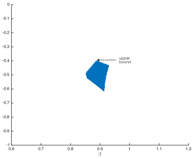
Figure 1: Identified Set: Entry Game

Using the specification above and instrument functions $1\{Z_{i}=z_{k}\},k=1,\cdots,K$, we transform the conditional moment inequalities in (10)-(11) into the following unconditional moment inequalities:

$$E\big{[}\big{(}1\{Y_{i}=(0,1)\}-H_{1}(Z_{i};\theta)\big{)}1\{Z_{i}=z_{k}\}\big{]} \leq 0$$ (22)

$$E\big{[}\big{(}H_{2}(Z_{i};\theta)-1\{Y_{i}=(0,1)\}\big{)}1\{Z_{i}=z_{k}\}\big{]} \leq 0,$$

where the entry probabilities

$$H_{1}(Z_{i};\theta) \equiv P(u_{1}\leq-Z_{1,i}^{\prime}\beta_{1}-\Delta_{1},~{}u_{2}>-Z_{2,i}^{\prime}\beta_{2}|Z_{i})$$ (23)

$$H_{2}(Z_{i};\theta) \equiv P(u_{1}\leq-Z_{1,i}^{\prime}\beta_{1}-\Delta_{1},u_{2}>-Z_{2,i}^{\prime}\beta_{2}-\Delta_{2}|Z_{i})$$

$$\qquad\qquad+P(u_{1}\leq-Z_{1,i}^{\prime}\beta_{1},-Z_{2,i}^{\prime}\beta_{2}\leq u_{2}\leq-Z_{2,i}^{\prime}\beta_{2}-\Delta_{2}|Z_{i})$$ (24)

are calculated using either an analytical expression or a frequency simulator. For example, using the parametric specification, $H_{1}(Z_{i},\theta)$ may be computed analytically as $\Phi(-Z_{1,i}^{\prime}\beta)\times\Phi(Z_{2,i}^{\prime}\beta)$. Alternatively, using a simulator one may compute the same object as $R^{-1}\sum_{r=1}^{R}1\{u_{1,i,r}\leq-Z_{1,i}\beta,u_{2,i,r}>-Z_{2,i}\beta\}$, where $(u_{1,i,r},u_{2,i,r}),r=1,\cdots,R$ are drawn from the bivariate standard normal distribution.

Our benchmark inference procedure is implemented as follows. The confidence region takes the form: $CS_{n}=\{\theta\in\Theta:T_{n,R}(\theta)\leq c_{n}(\theta)\}$, where $T_{n,R}$ is the statistic proposed by Rosen (2008) and further refined by Andrews & Barwick (2012):

$$T_{n,R}(\theta)=\inf_{t\in\mathbb{R}_{+}^{J}}(\sqrt{n}\bar{m}_{n,R}(\theta)-t)^{\prime}\tilde{\Sigma}_{n,R}^{-1}(\theta)(\sqrt{n}\bar{m}_{n,R}(\theta)-t),$$

where $\tilde{\Sigma}_{n,R}$ is a suitable estimator of the asymptotic variance of the moments. The critical value $c_{n}(\theta)$ is computed using a bootstrap procedure combined with the generalized moment selection (GMS) procedure (Andrews & Soares, 2010; Andrews & Barwick, 2012). For details on the GMS procedure, we refer to the references above, but we briefly describe its mechanism to highlight the potential effects of simulation on this procedure. The key idea of the GMS is to compute the critical value by selecting the moments that are relevant to the asymptotic null distribution of the test. For example, in an implementation of the GMS, the $j$-th moment inequality is “selected” and used to calculate $c_{n}$ if the studentized moment is smaller than a tuning parameter $\kappa_{n}$, i.e. $\frac{\sqrt{n}\bar{m}_{j,n,R}(\theta)}{\hat{\sigma}_{j,n,R}(\theta)}\leq\kappa_{n}$, where $\hat{\sigma}_{j,n,R}^{2}(\theta)$ is the $j$-th diagonal element of $\hat{\Sigma}_{n,R}(\theta)$. The critical value is then computed as the $1-\alpha$ quantile of the bootstrapped statistic where the sample moments are replaced with the bootstrap analog of the selected moments. We note here that the simulated moments could also potentially affect the GMS step, but its consequence is not immediately clear.

Table 3: Coverage Probabilities for $\theta^{U}$

	Analytical	Simulated
		$R=1$	$R=5$	$R=10$	$R=20$
Panel A: ($n=250$)
Coverage prob	$0.921$	$0.391$	$0.453$	$0.449$	$0.454$
$\#$ of times differ in selection		$997$	$858$	$755$	$666$
Panel B: ($n=500$)
Coverage prob	$0.945$	$0.814$	$0.903$	$0.906$	$0.909$
$\#$ of times differ in selection		$979$	$766$	$587$	$448$
Panel C: ($n=1000$)
Coverage prob	$0.961$	$0.833$	$0.947$	$0.952$	$0.960$
$\#$ of times differ in selection		$982$	$800$	$638$	$475$
Panel D: ($n=2000$)
Coverage prob	$0.953$	$0.756$	$0.935$	$0.941$	$0.949$
$\#$ of times differ in selection		$990$	$831$	$709$	$539$

Table 3 reports simulation results based on sample size $n\in\{250,500,1000,2000\}$ and the number of simulation draws $R=\{1,5,10,20\}$. We simulate $1000$ datasets for each setting. The coverage probabilities of the confidence regions with nominal level $95\%$ are evaluated for the true upper bound $\theta^{U}$.

The main finding is that, for small sample size and simulation size, the coverage probabilities of the confidence region are distorted in a significant way. In particular, with $n=250$, the coverage probabilities of the simulation-based confidence regions vary from 39.1% to 45.3%, significantly below the nominal level. Even for a moderate sample size, these confidence regions exhibit size distortions when the number of draws $R$ is small. For example, for $n=2000$, the coverage probabilities of the simulated-based confidence region is 75.6% when only a single draw is used. However, this gets improved (to 93.5%) with $R=5$ draws. Table 3 suggests that, with $R=20$, the coverage probabilities of simulation based confidence regions are close to those of of the analytical ones in relatively large samples ($n=1000,2000$).

This experiment suggests that the test statistic may not be able to benefit from averaging of the simulation errors when the number of observations in each bin is small. Combined with the irregular nature of the test statistic, this can result in a severe size distortion. The presence of bins with small numbers of observations is common in empirical settings. In such cases, care must be taken. One possibility may be to increase the number of simulation draws for such bins. However, the choice of the number of draws becomes an arbitrary component of inference. Another possibility is to modify the procedure to explicitly account for the effects of the simulation. In the next section, we explore several possibilities along this line.

As a final remark, we note that the simulation not only affects the value of the test statistic but also the general moment selection procedure. Table 3 reports the number of times (out of 1000) the set of the selected moments differ between the simulated and analytical methods. This difference arises because the simulation adds perturbation to the studentized moment. With a limited number of draws, this effect on the GMS may not be negligible. As a result, some of the “selected” inequalities (i.e. $\sqrt{n}\bar{m}_{j,n}(\theta)/\hat{\sigma}_{j,n}(\theta)\geq-\kappa_{n}$) according to the GMS based on the analytical moment may be discarded (i.e. $\sqrt{n}\bar{m}_{j,n,R}(\theta)/\hat{\sigma}_{j,n,R}(\theta)<-\kappa_{n}$) under the GMS based on the simulated moment, and vice versa.

3 Inference methods with corrections for simulation errors

We consider two methods to account for the simulation errors. One is to correct the critical value. The other is to correct or “regularize” the test statistic. The former method closely follows the recent development on the moment inequality literature, and hence we keep its discussion minimal. The second method is a novel approach and has several attractive features for simulation based methods. It combines a simple bias correction method with a bootstrap critical value based on a regular (and differentiable) functional of a random vector that is asymptotically normal. To our knowledge, the uniform validity of such a method in the context of simulation-based inference is new to the literature.

3.1 Critical value correction methods

Commonly used inference methods provide approximations to the distribution of the test statistic in (26). Many of these methods are based on resampling techniques. As we saw in the previous section, ignoring the variation due to simulation can result in poor inference. Recall that, in the numerical experiment in Section 2.2, the size distortion occurred because the naive critical value did not take into account the bias that was due to the extra variation from the approximation error $\frac{1}{n}\sum_{i=1}^{n}r_{j,i}$ (in (16)). A straightforward way to correct this effect is to adjust the critical value. One can achieve this by a bootstrap critical value that resamples the simulated variables $u_{i,r}$ along with the original sample $X_{i}$ across bootstrap replications. Specifically, let $\{X^{*}_{i},i=1,\dots,n\}$ be a bootstrap sample drawn with replacement from the empirical distribution. For each $i$, let $\{u^{*}_{i,r},r=1,\dots,R\}$ be drawn from $P(\cdot|X^{*}_{i})$.

We then let $\hat{m}^{*}_{R}(W^{*}_{i},\theta)=R^{-1}\sum_{r=1}^{R}M(X^{*}_{i},u^{*}_{i,r},\theta)$ be the simulation approximation to the (conditional) moment function in the $i$-th bootstrap sample. Define

$$\bar{m}^{*}_{n,R}(\theta)\equiv\frac{1}{n}\sum_{i=1}^{n}\hat{m}^{*}_{R}(W^{*}_{i},\theta).$$ (25)

This resampled moment is constructed so that it mimics the behavior of $\bar{m}_{n,R}$ including the variation due to the simulated variables. The final step is to use the resampled moment above when one applies an existing method for computing the critical value. For example, consider the generalized moment selection (GMS) in Andrews & Soares (2010). Let $\hat{D}_{n,R}(\theta)=\text{diag}(\hat{\Sigma}_{n,R}(\theta))$ and let $\hat{\Omega}_{n,R}(\theta)$ be an estimator of the correlation matrix, i.e. $\hat{\Omega}_{n,R}(\theta)=\hat{D}_{n,R}(\theta)^{-1/2}\hat{\Sigma}_{n,R}(\theta)\hat{D}_{n,R}(\theta)^{-1/2}.$ This procedure uses the $1-\alpha$ quantile $c_{\kappa,n,R}(\theta)$ of the following statistic

$$T^{*}_{n,R}(\theta)=S\big{(}\hat{D}_{n,R}(\theta)^{-1/2}Z^{*}_{n,R}(\theta)+\varphi(\xi_{n,R}(\theta)),\hat{\Omega}_{n,R}(\theta)\big{)},$$ (26)

where $Z^{*}_{n,R}(\theta)=\sqrt{n}(\bar{m}^{*}_{n,R}(\theta)-\bar{m}_{n,R}(\theta))$ is the bootstrapped empirical process, and $\xi_{n,R}$ is a $J\times 1$ vector whose components are

$$\xi_{j,n,R}(\theta)\equiv\kappa_{n}^{-1}\sqrt{n}\frac{\bar{m}_{j,n,R}(\theta)}{\hat{\sigma}_{j,n,R}(\theta)},~{}j=1,\dots,J.$$ (27)

The generalized moment selection (GMS) function $\varphi$ then selects the inequalities that are relevant for the inference for $\theta$ based on $\xi_{n,R}$ (see Andrews & Soares (2010) for details). The resulting confidence region is

$$\mathcal{C}_{n,R}^{\text{CV}}=\{\theta\in\Theta:T_{n,R}(\theta)\leq c_{\kappa,n,R}(\theta)\}.$$ (28)

In Example 1, applying this method with a $t$-test based GMS function ($\varphi(\xi_{j})=0$ if $\xi_{j}\geq-1$ and $=-\infty$ otherwise) yields the following confidence interval

$$\mathcal{C}_{n,R}^{\text{CV}}=\Big{\{}\theta\in\mathbb{R}:\sqrt{n}\max\Big{\{}\frac{\bar{m}_{1,n,R}(\theta)}{\hat{\sigma}_{1,n,R}},\frac{\bar{m}_{2,n,R}(\theta)}{\hat{\sigma}_{2,n,R}}\Big{\}}\leq c_{\kappa,n,R}\Big{\}}\\ =\Big{(}-\infty,\min_{j=1,2}\Big{\{}\frac{1}{nR}\sum_{i=1}^{n}\sum_{r=1}^{R}1\{u_{j,i,r}<X_{j,i}\}+c_{\kappa,n,R}\frac{\hat{\sigma}_{j,n,R}}{\sqrt{n}}\Big{\}}\Big{]},$$ (29)

where the critical value $c_{\kappa,n,R}$ is the $1-\alpha$ quantile of the bootstrapped statistic

$$T^{*}_{n,R}(\theta) \equiv\max_{j\in\{j:\xi_{j,n,R}\geq-1\}}\frac{\sqrt{n}(\bar{m}^{*}_{j,n,R}(\theta)-\bar{m}_{j,n,R}(\theta))}{\hat{\sigma}_{j,n,R}}$$

$$=\max_{j\in\{j:\xi_{j,n,R}\geq-1\}}\frac{\frac{1}{\sqrt{n}R}\sum_{i=1}^{n}\sum_{r=1}^{R}1\{u^{*}_{j,i,r}<X^{*}_{j,i}\}-1\{u_{j,i,r}<X_{j,i}\}}{\hat{\sigma}_{j,n,R}}.$$ (30)

The confidence interval in this example is the intersection of the sample (upper) bounds that are suitably expanded. The amount of the expansion $c_{\kappa,n,R}\frac{\hat{\sigma}_{j,n,R}}{\sqrt{n}}$ accounts for the variation of each simulated moment. This type of confidence interval is also considered in the context of conditional moment restrictions in Chernozhukov et al. (2013).

Remark 3.1.

The method described above accounts for the simulation variation contained in the sample moment $\bar{m}_{n,R}$. Hence, one can expect that it mitigates the problem we saw in Section 2.2. However, it does not account for the second channel through which simulation can affect the performance of the confidence region. This is through the rescaled moments $\xi_{j,n,R},j=1,\cdots,J$ used in the GMS function. As we saw in Table 3, the effect of simulation on the selected set of moments is nontrivial. However, since the critical value may depend on $\xi_{n,R}$ in a discontinuos manner (see the $t$-test based on GMS above), the analysis of the effect of the simulation error on the coverage probability through this channel is complex. We therefore do not pursue the correction of the effect of simulation through $\xi_{n,R}$. In contrast, our alternative inference method in the next section admits a straightforward way to correct the effect of simulation.

3.2 Regularization of test statistics

In addition to the modification of the existing methods, we propose a novel and computationally simple inference procedure that accounts for simulation. The key idea is as follows. Recall that commonly used test statistics take the form: $T_{n,R}(\theta)=S(\sqrt{n}\bar{m}_{n,R}(\theta),\hat{\Sigma}_{n,R}(\theta))$ whose irregular behavior arises due to the non-smoothness of $S$. Our procedure replaces $S$ by a smooth approximation $S_{\mu}$, which satisfies certain regularity conditions. This approach has several attractive features. First, the proposed method has a uniform approximation property. That is, for any $(m,\Sigma)$, $|S_{\mu}(m,\Sigma)-S(m,\Sigma)|\leq\beta\mu$ for a known uniform constant $\beta$ and the degree of smoothness $\mu>0$, which is chosen by the researcher. Accounting for the approximation error is then straightforward because $\beta$ is known. Second, the approximated test statistic $\tilde{T}_{n,R}(\theta)\equiv S_{\mu}(\sqrt{n}\bar{m}_{n,R}(\theta),\hat{\Sigma}_{n,R}(\theta))$ obeys standard limit theorems uniformly over a large class of DGPs and over a range of values for $\mu$. This in turn allows one to employ a standard resampling method such as bootstrap to calculate the critical value. Finally, smooth approximations to a wide class of non-smooth convex functions are available thanks to the recent developments in the non-smooth convex optimization literature (see e.g. Nesterov, 2005; Beck & Teboulle, 2012). Using these results, we provide functional forms of smooth approximations to some of the commonly used test statistics. The idea of regularizing test statistics (or estimated bounds) also appears in related contexts (Haile & Tamer, 2003; Chernozhukov et al., 2015; Kaido, 2017; Masten & Poirier, 2017). Our contribution here is to show its uniform validity in the context of inference with simulated variables. A potential price for this computationally simple method is the possibility of inference becoming conservative for some choice of the smoothing parameter. We will examine this point numerically in Section 4.

Below, we illustrate our approach using Example 1.

Example 1 (Intersection bounds (continued)).

Recall the confidence interval in (7):

$$\mathcal{C}_{n,R}^{\text{Sim}} =\{\theta:S\big{(}\sqrt{n}(\bar{m}_{1,n,R}(\theta),\bar{m}_{2,n,R}(\theta))^{\prime},\hat{\Sigma}_{n,R}(\theta)\big{)}\leq c_{n,R}\},$$ (31)

where $S((m_{1},m_{2})^{\prime},\Sigma)=\max\{m_{1},m_{2}\}$. Consider replacing $S$ with a smooth approximation. Specifically, for $\mu>0$, define

$$\tilde{\mathcal{C}}_{n,R}=\{\theta:S_{\mu}\big{(}\sqrt{n}(\bar{m}_{1,n,R}(\theta),\bar{m}_{2,n,R}(\theta)),\hat{\Sigma}_{n,R}(\theta)\big{)}\leq\tilde{c}_{\mu,n,R}\},$$ (32)

where $S_{\mu}((m_{1},m_{2})^{\prime},\Sigma)\equiv\mu\ln(\exp(\frac{m_{1}}{\mu})+\exp(\frac{m_{2}}{\mu}))$ replaces the maximum function. We then calculate our critical value $\tilde{c}_{\mu,n,R}$ by

$$\tilde{c}_{\mu,n,R}=c_{1-\alpha,R}+\sqrt{n}\mu\ln 2.$$ (33)

This critical value consists of two terms. The first term, $c_{1-\alpha,R}$, is an approximation to the $1-\alpha$ quantile of the root (centered and rescaled statistic):

$$Z_{n}=\sqrt{n}\big{(}S_{\mu}((\bar{m}_{1,n,R}(\theta),\bar{m}_{2,n,R}(\theta))^{\prime},\hat{\Sigma}_{n,R}(\theta))-S_{\mu}((E_{P}[m_{1}(X_{i},\theta)],E_{P}[m_{2}(X_{i},\theta)])^{\prime},\Sigma_{P}(\theta))\big{)}.$$ (34)

The second term in (33) is a bias-correction term that accounts for the approximation error (or population-level bias) that arises when we replace $S(E_{P}[m(X_{i},\theta)],\Sigma_{P}(\theta))$ by its smooth counterpart $S_{\mu}(E_{P}[m(X_{i},\theta)],\Sigma_{P}(\theta))$. The quantile $c_{1-\alpha,R}$ can be approximated by a bootstrap procedure that resamples an analog of $Z_{n}$ in (34) (see Algorithm 1 below).

The confidence interval in (32) is asymptotically valid over a wide class of data generating processes and choices of $\mu$. We sketch the argument below and defer the formal proof to the sequel.

Let $\theta=\min\{E_{P}[\Phi(X_{1,i})],E_{P}[\Phi(X_{2,i})]\}$ be the upper boundary point of the identified set. Then, $S(E_{P}[m(X_{i},\theta)],\Sigma_{P}(\theta))=0.$ Let $0<\underline{M}<\overline{M}<\infty.$ Then, uniformly in $\mu\in[\underline{M},\overline{M}]$ and in $P$ over a class of distributions specified below, the (least favorable) coverage probability is

$$P (\theta\in\tilde{\mathcal{C}}_{n,R})$$

$$=P\big{(}S_{\mu}\big{(}\sqrt{n}(\bar{m}_{1,n,R}(\theta),\bar{m}_{2,n,R}(\theta)),\hat{\Sigma}_{n,R}(\theta)\big{)}\leq\tilde{c}_{\mu,n,R})$$ (35)

$$=P\big{(}Z_{n}-\sqrt{n}(S_{\mu}(E_{P}[m(X_{i},\theta)],\Sigma_{P}(\theta))-S(E_{P}[m(X_{i},\theta)],\Sigma_{P}(\theta)))\leq\tilde{c}_{\mu,n,R}\big{)}$$

$$\geq P(Z_{n}+\sqrt{n}\mu\ln 2\leq\tilde{c}_{\mu,n,R})$$

$$=P(Z_{n}\leq c_{1-\alpha,R})\to 1-\alpha,$$ (36)

where we used (34), $|S_{\mu}(m)-S(m)|\leq\beta\mu$ with $\beta=\ln 2$ (see Table 4). The convergence in the last step follows from the argument below.

Note that $S_{\mu}$ is differentiable with the following derivative:

$$DS_{\mu}[m](h)=\sum_{j=1}^{2}w_{j}(m,\mu)h_{j},~{}w_{j}(m,\mu)=\frac{e^{m_{j}/\mu}}{\sum_{j=1}^{2}e^{m_{j}/\mu}}.$$ (37)

It can be shown that $DS_{\mu}$ is Lipschitz continuous in $m$ with a Lipschitz constant $\mu^{-1}.$ Hence, by the mean-value theorem,

$$Z_{n} =DS_{\mu}[\bar{m}_{n,R}^{*}](\sqrt{n}(\bar{m}_{n,R}-E_{P}[m(X_{i})]))$$ (38)

$$=DS_{\mu}[E_{P}[m(X_{i})]]\sqrt{n}(\bar{m}_{n,R}-E_{P}[m(X_{i})])+\frac{1}{\mu}r_{n},$$ (39)

where $r_{n}=o_{P}(1)$ uniformly in $P$ as $n\to\infty$ with $R$ fixed. Hence, $Z_{n}$ converges in distribution to some limit $Z$ uniformly in $\mu$ over a compact set (not containing 0).

Now, let us compare this to a method without any regularization of $S$. The coverage probability of the confidence interval in (31) is

$$P(\theta\in\mathcal{C}_{n,R}^{\text{Sim}}) =P\big{(}\sqrt{n}(S(\bar{m}_{n,R}(\theta),\hat{\Sigma}_{n,R}(\theta))-S(E_{P}[m(X_{i},\theta)],\Sigma_{P}(\theta)))\leq c_{n,R}\big{)},$$ (40)

The transformation $S$ is not differentiable but can be shown to be directionally differentiable with the following directional derivative:

$$DS[m](h)=\min_{j\in\mathcal{J}^{*}(m)}h_{j},~{}\mathcal{J}^{*}(m)=\{j:m_{j}=\min\{m_{1},m_{2}\}\}.$$ (41)

Observe that the directional derivative is non-linear in $h$ (but only positively homogeneous). More importantly, the directional derivative depends on $m$ and hence the underlying data generating process in a discontinuous manner. This is because the set of “active” inequalities, $\mathcal{J}^{*}(m)$, depends on $m$ discontinuously. This in turn implies that the limiting distribution of the test statistic is discontinuous in the underlying DGP. Hence, a small perturbation of the underlying data generating process may result in a significant change in the distribution of the statistic. When simulation is used to replace the population moments, this therefore could affect the behavior of the statistic in non-trivial ways. This feature motivated the vast literature on moment inequalities that corrects the critical value whenever this type of discontinuity is a concern (see e.g Andrews & Soares, 2010; Chernozhukov et al., 2013; Fang & Santos, 2014; Romano et al., 2014).

In contrast, our approach first replaces the $S(\bar{m}_{n,R}(\theta),\hat{\Sigma}_{n,R}(\theta))$ by a smooth approximation $S_{\mu}(\bar{m}_{n,R}(\theta),\hat{\Sigma}_{n,R}(\theta))$, while correcting for the population level bias. Since the limiting distribution of $S_{\mu}(\bar{m}_{n,R}(\theta),\hat{\Sigma}_{n,R}(\theta))$ depends on the underlying distribution in a smooth manner, there is no need to correct the critical value $c_{1-\alpha,R}$. In short, our approach regularizes the behavior of the statistic, while the vast literature regularizes the critical value to ensure the uniform validity of inference.

The motivations for this approach are two-fold. First, it is straightforward to show that the proposed method is uniformly valid under the large $n$ asymptotics with a fixed simulation size $R$. The proposed method combines the standard $\delta$-method with a bias correction (at the population level). The method and its uniform validity may be of independent interest outside the context of simulation based inference. Second, the inference method is simple and can be implemented by a standard bootstrap procedure. This is attractive as accounting for the effects of simulation errors on moment selection procedures or Bonferroni-correction methods in the existing literature may be non-trivial.

In general, we define our confidence set by

$$\tilde{\mathcal{C}}_{n,R}\equiv\{\theta:\tilde{T}_{n,R}(\theta)\leq\tilde{c}_{n,R}(\theta)\},$$ (42)

where the test statistic and the critical value are calculated as follows

$$\tilde{T}_{n,R}(\theta) \equiv S_{\mu}(\sqrt{n}\bar{m}_{n,R}(\theta),\hat{\Sigma}_{n,R}(\theta)),$$ (43)

$$\tilde{c}_{n,R}(\theta) \equiv c_{n,R,1-\alpha}(\theta)+\sqrt{n}\mu\beta,$$ (44)

where $c_{n,R,1-\alpha}$ is an estimate of the $1-\alpha$ quantile of

$$Z_{\mu,n,R}=S_{\mu}(\sqrt{n}\bar{m}_{n,R}(\theta),\hat{\Sigma}_{n,R}(\theta))-S_{\mu}(\sqrt{n}E_{P}[m(X_{i},\theta)],\Sigma(\theta)).$$ (45)

Here, $S_{\mu}$ is an approximation to $S$, which has smoothness properties that are useful for analyzing and correcting the behavior of the test statistic in the presence of simulated variables. We introduce the following notion of approximation based on Beck & Teboulle (2012).

Definition 3.1 ($\mu$-smooth approximation).

Let $\phi:\mathbb{R}^{J}\to(-\infty,\infty]$ be a closed and proper convex function and let $M\subseteq\text{dom}(\phi)$ be a closed convex set. A function $\phi_{\mu}:\mathbb{R}^{J}\to(-\infty,\infty)$ is said to be a $\mu$-smooth approximation of $\phi$ with parameters $(\alpha,\beta,K)$ if the following conditions hold:

(i) $\phi(m)-\beta_{1}\mu\leq\phi_{\mu}(m)\leq\phi(m)+\beta_{2}\mu$ for some $\beta_{1},\beta_{2}$ satisfying $\beta_{1}+\beta_{2}=\beta>0$;

(ii) $\phi_{\mu}$ has a derivative $D\phi_{\mu}[m](\cdot)$ such that

$$\big{\|}D\phi_{\mu}[m]-D\phi_{\mu}[m^{\prime}]\big{\|}^{*}\leq(K+\frac{\alpha}{\mu})\|m-m^{\prime}\|,~{}\forall m,m^{\prime}\in M,$$ (46)

for some $K\geq 0$ and $\alpha>0$;

(iii) For each $m$, $(\mu,h)\mapsto D\phi_{\mu}[m](h)$ is continuous.

Definition 3.1 (i) requires that $\phi_{\mu}$ has a uniform approximation property, which is the key condition for bias correction. Definition 3.1 (ii) requires that $\phi_{\mu}$’s derivative is Lipschitz continuous, which plays a role in making the limiting distribution of $Z_{\mu,n,R}$ depend continuously on the underlying DGP. Given this definition, we require $S$ and $S_{\mu}$ to satisfy the following condition. For this, let $\mathbb{P}^{J}$ be the set of $J\times J$ symmetric positive semi-definite matrices.

Assumption 3.1.

(i) The index function $S:\mathbb{R}^{J}\times\mathbb{P}^{J}\to\mathbb{R}_{+}$ satisfies Assumptions $1-6$ in Andrews & Soares (2010). For any $a>0$ and $(m,\Sigma)\in\mathbb{R}^{J}\times\mathbb{P}^{J}$, $S(am,\Sigma)=a^{\chi}\phi(V^{-1/2}m)$ for a proper convex function $\phi:\mathbb{R}^{J}\to\mathbb{R}_{+}$ with $\chi=1$, where $V=\text{diag}(\Sigma)$; (ii) For each $\mu\in[\underline{M},\overline{M}]$, the map $S_{\mu}:\mathbb{R}^{J}\times\mathbb{P}^{J}\to\mathbb{R}_{+}$ is such that for any $a>0$ and $(m,\Sigma)\in\mathbb{R}^{J}\times\mathbb{P}^{J}$, $S_{\mu}(am,\Sigma)=a^{\chi}\phi_{\mu}(V^{-1/2}m)$ for a $\mu$-smooth approximation $\phi_{\mu}$ of $\phi$.

In what follows, we also call $S_{\mu}$ the $\mu$-smooth approximation of $S$. Table 4 gives the index functions we consider and their $\mu$-smooth approximations with associated parameters. Details are provided in Appendix A. These functions satisfy Assumption 3.1.

Table 4: $\mu$-smooth approximations of commonly used index functions.

	$S(m,\Sigma)$	$S_{\mu}(m,\Sigma)$	$(\alpha,\beta,K)$
(i)	$\sum_{j=1}^{J}[m_{j}/\sigma_{j}]_{+}$	$\mu\sum_{j=1}^{J}\ln(\exp(\frac{m_{j}}{\mu\sigma_{j}})+1)$	$(J,J\ln 2,0)$
(ii)	$\max_{j=1,\cdots,J}\{m_{j}/\sigma_{j}\}_{+}$	$\mu\ln(\sum_{j=1}^{J}\exp(\frac{m_{j}}{\mu\sigma_{j}})+1)$	$(1,\ln(J+1),0)$

In summary, we propose the following procedure to construct confidence regions.

Algorithm 1:

Step 1

: Choose $\mu>0$. Calculate $\tilde{T}_{n,R}(\theta)$ using a $\mu$-smooth approximation $S_{\mu}$ of $S$ in Table 4 and simulated samples of size $R$. For each observation $X_{i^{\prime}}$, also draw a larger simulated sample $\{u_{i^{\prime},1},\cdots,u_{i^{\prime},R_{2}}\}$ with $R\ll R_{2}$ from the law $P(\cdot|X_{i^{\prime}})$ for $i^{\prime}=1,\cdots,n$.

Step 2

: Bootstrap.

• Let $\{X^{*}_{1},\cdots,X^{*}_{n}\}$ be drawn from the empirical distribution of $\{X_{1},\cdots,X_{n}\}$ (with replacement).

• For each bootstrapped observation $X^{*}_{i}$, draw a simulated sample $\{u_{i,1},\cdots,u_{i,R}\}$ from the law $P(\cdot|X^{*}_{i})$ for $i=1,\cdots,n$.

• Compute the $1-\alpha$ quantile $c_{n,R,1-\alpha}(\theta)$ of the root:

  $$Z^{*}_{\mu,n,R,R_{2}}=\sqrt{n}(S_{\mu}(\bar{m}^{*}_{n,R},\hat{\Sigma}^{*}_{n,R})-S_{\mu}(\bar{m}_{n,R_{2}},\hat{\Sigma}_{n,R_{2}})).$$ (47)

Step 3

: Calculate the critical value $\tilde{c}_{n,R}(\theta)$ in (44) by introducing the correction term $\sqrt{n}\beta\mu$ for the approximation bias.

Step 4

: For each $\theta\in\Theta$, conduct steps 1-3 and report $\mathcal{\tilde{C}}_{n,R}=\{\theta\in\Theta:\tilde{T}_{n,R}(\theta)\leq\tilde{c}_{n,R}(\theta)\}.$

Similar to the consistent estimation of the asymptotic covariance matrix in the MSM literature, we use a simulation sample of larger size in the algorithm (see e.g. Gourieroux & Montfort, 1996, Section 2.3). This is to re-center the bootstrapped root at an object that tends to the population counterpart and mimic the behavior of the root in (45) by the bootstrap sample. While $R_{2}$ needs to be large for the asymptotic approximation to be valid, this simulation needs to be done only once.

Below, we establish the asymptotic validity of the inference procedure described above. For each $j$, we let $\sigma^{2}_{P,j}(\theta)\equiv Var_{P}(\hat{m}_{j,R}(X_{i},u_{i},\theta))$ and $\Omega_{P}(\theta)\equiv Corr_{P}(\hat{m}_{j,R}(X_{i},u_{i},\theta))$, where $\hat{m}_{j,R}(X_{i},u_{i},\theta)=R^{-1}\sum_{r=1}^{R}M_{j}(X_{i},u_{i,r},\theta)$. We then let $DS_{\mu}$ denote the gradient of the map $m\mapsto S_{\mu}(m,\Sigma).$ Let $\Psi$ be the set of $J$-by-$J$ correlation matrices $\Omega$ with $\det(\Omega)>\epsilon$ for some $\epsilon>0$. We make the following assumption on the model.

Assumption 3.2.

The model $\mathcal{F}$ for $(\theta,P)$ satisfies the following conditions.

(i) $\theta\in\Theta;$

(ii) $E_{P}[m_{j}(X_{i},\theta)]\leq 0,j=1,\cdots,J$ for some $\theta\in\Theta;$

(iii) $\{X_{i},u_{i,1},\cdots,u_{i,R},i=1,\cdots,n\}$ is an i.i.d. sample from $P$;

(iv) $\sigma_{P,j}(\theta)\in(0,\infty)$ for $j=1,\cdots,J$ and $\theta\in\Theta$;

(v) $\Omega_{P}(\theta)\in\Psi$;

(vi) $E_{P}\Big{[}\Big{|}\frac{m_{j}(X_{i},\theta)}{\sigma_{P,j}(\theta)}\Big{|}^{2+\delta}\Big{]}\leq M$ for some $\delta>0$ and $0<M<\infty$;

(vii) For any $\mu\in[\underline{M},\overline{M}]$, $\|DS_{\mu}(E_{P}[m(X_{i},\theta)],\Sigma_{P}(\theta))\|\geq\eta$ for some $\eta>0$ and for all $\theta\in\Theta$.

Assumption 3.2 (i)-(vi) are based on the conditions in Andrews & Guggenberger (2009); Andrews & Soares (2010). In (iii), we assume an i.i.d. sample. With this assumption, the following estimator of the asymptotic covariance can be used:

$$\hat{\Sigma}_{n,R}(\theta)=\frac{1}{n}\sum_{i=1}^{n}(\hat{m}_{R}(X_{i},\theta)-\bar{m}_{n,R}(\theta))(\hat{m}_{R}(X_{i},\theta)-\bar{m}_{n,R}(\theta))^{\prime}.$$ (48)

We then let $\hat{V}_{n,R}(\theta)=\text{diag}(\hat{\Sigma}_{n,R}(\theta))$. For the purpose of stating an assumption, let us also define an infeasible estimator of $\Sigma_{P}$ as follows:

$$\hat{\Sigma}_{n}(\theta)=\frac{1}{n}\sum_{i=1}^{n}(m(X_{i},\theta)-\bar{m}_{n}(\theta))(m(X_{i},\theta)-\bar{m}_{n}(\theta))^{\prime}.$$

This estimator can be computed only if simulation is not required. We then let $\hat{V}_{n}(\theta)=\text{diag}(\hat{\Sigma}_{n}(\theta))$.

In Assumption 3.2 (v), $\Psi$ contains all $J\times J$ correlation matrices whose determinant is bounded from below by $\epsilon>0$. This condition is required for one of the index functions used in Andrews & Soares (2010). In our setting, we use this condition to ensure that the limiting distribution of $Z_{\mu,n,R}$ is continuously distributed. With additional notation, this assumption can be relaxed so that the lower bound on the determinant is required only for the correlation matrix of a suitable subset of the moment functions. Or it can be dropped entirely at the price of an additional tuning parameter to handle a potentially discontinuos limiting distribution.

Assumption 3.2 (vii) is an additional condition, which we add to the standard set of assumptions. It requires that the gradient of the smoothed index function $S_{\mu}$ does not vanish. This allows us to use the (first-order) $\delta$-method. For the functions in Table 4, the condition is satisfied when $\theta\mapsto E_{P}[m_{j}(X_{i},\theta)]$ is continuous and $\sigma_{P,j}(\theta),j=1,\cdots,J$ are uniformly bounded away from 0.

The following theorem ensures that the proposed confidence region controls the asymptotic confidence size uniformly over the parameter space $\mathcal{F}$.

Theorem 3.1.

Suppose Assumptions 3.1-3.2 hold. Let $0<\underline{M}<\overline{M}<\infty$. Let $R\in\mathbb{N}$ be fixed and let $\{R_{2}\}\subset\mathbb{N}$ be a sequence such that $R_{2}\to\infty$ as $n\to\infty$ and $\hat{V}_{n,R_{2}}(\theta_{n})^{-1/2}\bar{m}_{n,R_{2}}(\theta_{n})-\hat{V}_{n}(\theta_{n})^{-1/2}\bar{m}_{n}(\theta_{n})=o_{P}(n^{-1/2})$ uniformly in $P$. Then,

$$\liminf_{n\to\infty}\inf_{\mu\in[\underline{M},\overline{M}]}\inf_{(\theta,P)\in\mathcal{F}}P\Big{(}\theta\in\tilde{\mathcal{C}}_{n,R}\Big{)}\geq 1-\alpha.$$

4 Monte Carlo Experiments

In this section, we show results of main Monte Carlo simulations to examine the performance of the methods that account for the simulation error.

4.1 Performance of methods with correction for simulation errors

Following our example on the intersection bounds in Section 2.2, we first use the method that corrects the critical value described in Section 3.1. We construct confidence intervals for $\theta$ with level $1-\alpha$ using:

$$\mathcal{C}_{n,R}^{\text{CV}} \equiv\big{(}-\infty,~{}\min_{j}\{\bar{m}_{j,n,R}+c_{\kappa,n,R}\frac{\hat{\sigma}_{j,n,R}}{\sqrt{n}}\big{\}}\big{]},$$ (49)

where $\bar{m}_{j,n,R}=(nR)^{-1}\sum_{i=1}^{n}\sum_{r=1}^{R}1\{u_{j,i,r}<X_{j,i}\},$ $\hat{\sigma}_{j,n,R}$ is the estimated standard deviation of the $j$-th simulated moment, and $c_{\kappa,n,R}$ is a critical value computed as the $1-\alpha$ quantile of

$$T^{*}_{n,R}=\max_{j\in\{j:\xi_{j,n,R}\geq-1\}}\sqrt{n}(\bar{m}_{j,n,R}^{*}-\bar{m}_{j,n,R})/\hat{\sigma}_{j,n,R}^{*},$$ (50)

where $(\bar{m}_{j,n,R}^{*},\hat{\sigma}_{j,n,R}^{*})$ is the bootstrap quantities corresponding to $(\bar{m}_{j,n,R},\hat{\sigma}_{j,n,R})$, and $\xi_{j,n,R}$ is as defined in (27) with $\kappa_{n}=\sqrt{\ln n}$. When $T^{*}_{n,R}$ is computed, we redraw simulation draws $\{u_{i,r},r=1,...R\}$ to account for simulation variations when simulating the bootstrap samples.

We also consider our inference procedure based on the regularized statistic. Specifically, we use $\phi_{\mu}(\bar{m}_{j,n,R})=-\mu\ln\sum_{j=1}^{J}e^{-\bar{m}_{j,n,R}/\mu}$ to approximate $\phi(\bar{m}_{j,n,R})=\min_{j=1,..J}\bar{m}_{j,n,R}$ used in computing the confidence region in equation (15). We then construct confidence intervals for $\theta$ with level $1-\alpha$ using:

$$\tilde{\mathcal{C}}_{n,R} \equiv\big{(}-\infty,\phi_{\mu}(\bar{m}_{j,n,R})+\tilde{c}_{\mu,n,R}/\sqrt{n}\big{]},$$ (51)

where $\tilde{c}_{n,R}$ is an estimated critical value in (44). We also redraw simulation draws $\{u_{i,r},r=1,...R\}$ when simulating the bootstrap samples. In the experiments, we use $R_{2}=100$ to compute $(\bar{m}_{n,R_{2}},\hat{\Sigma}_{n,R_{2}})$ in the bootstrap step (Step 2 in Algorithm 1). For both confidence intervals, $S=1000$ Monte Carlo replications are generated.

Table 6 reports the probabilities of the confidence intervals covering the upper bound $\theta^{U}$ of the identified set using the critical value correction. The coverage probabilities of the confidence intervals are all above the nominal level after correcting the critical value. This can be contrasted with the coverage probabilities of the confidence intervals without any correction. The critical value correction method tends to make the confidence interval somewhat conservative when $R$ is small. In some cases, the coverage probability is very close to 1 and the corrected confidence interval is substantially longer than the one based on the regularization method as we discuss below.

Table 6 reports the coverage probabilities of the confidence intervals based on the $\mu$-smooth approximation. We set the smoothing parameter to $\mu=0.02$ and $0.04$ in our Monte Carlo experiments. The coverage probabilities of $\tilde{\mathcal{C}}_{n,R}$ are all above those of the confidence intervals without correction and close to the nominal level in many cases. These results indicate that the inference procedure with the $\mu$-smooth approximation is an effective method for correcting the size distortion caused by the finite number of draws.

Tables 8 and 8 report the median length of the confidence intervals. The median length of a one-sided confidence interval is computed as the difference between the median of the upper bound of the confidence interval and the right end point of the identified set. Table 8 shows that the confidence interval with the critical value correction is often much longer than the confidence interval without any correction, which is consistent with the robust size control property. The difference between the two shrinks as $R$ gets large. Comparing the two tables, one can see that the regularization based confidence intervals $\tilde{\mathcal{C}}_{n,R}$ are often significantly shorter than $\mathcal{C}_{n,R}^{\text{CV}}$. A close inspection of the simulation results showed that this was because the regularized statistic had a smaller variance that that of the non-regularized statistic, which led to shorter confidence intervals even after the bias correction.

The overall pattern remains the same even in the presence of locally slack constraints. Tables 10-12 report the coverage probabilities and excess length of the confidence intervals when some of the constraints are slack. The slack constraints are introduced by shifting $X_{j}$’s mean by $1/\sqrt{n}$ for the first $J/5$ constraints. One can see that both correction methods achieve valid coverage across all values of simulation draws. The regularization based confidence interval becomes slightly more conservative in terms of coverage probabilities compared to the case without the slack constraints. However, its length is still shorter than that of the critical value correction confidence interval across all cases.

In sum, the simulation results show that the regularization based confidence interval $\tilde{\mathcal{C}}_{n,R}$ works well both in terms of size and length. Its size is controlled reasonably well even under some DGPs that make simulated confidence intervals without correction severely undersized. The critical value correction method also achieves robust size control. However, it tends to be overly conservative when $R$ is small.

5 Concluding remarks

This paper explores the effects of simulated moments on the performance of inference methods based on moment inequalities. Due to the irregularity of the boundary of the confidence regions, simulation errors can affect the performance of inference in non-standard ways. This can result in a severe distortion especially when the number of inequality restrictions is large and the essential sample size is small. To account for the effect of the simulation error, we propose a novel way to construct confidence regions using regularized statistics and establish an asymptotic size control result. The simulation results confirm the robust size control property of the proposed method. An interesting avenue for future research is on the choice of the smoothing parameter that accounts for the trades-off between the amount of bias correction and variance of the regularized statistic.

Table 5: Coverage Probabilities for True Upper Bound: Critical Value Correction

	Simulated (No correction)					CV correction: $\mathcal{C}_{n,R}^{\text{CV}}$
	$R=1$	$R=5$	$R=10$	$R=20$		$R=1$	$R=5$	$R=10$	$R=20$
A: ($J=5$)
$n=100$	0.583	0.882	0.908	0.930		$0.998$	$0.977$	$0.959$	$0.954$
$n=250$	0.604	0.881	0.920	0.935		$0.998$	$0.969$	$0.968$	$0.965$
$n=1000$	0.666	0.894	0.913	0.933		$0.997$	$0.983$	$0.968$	$0.957$
B: ($J=10$)
$n=100$	0.481	0.853	0.904	0.920		$0.996$	$0.972$	$0.955$	$0.948$
$n=250$	0.467	0.868	0.908	0.925		$0.998$	$0.980$	$0.964$	$0.957$
$n=1000$	0.487	0.853	0.896	0.919		$1.000$	$0.983$	$0.963$	$0.951$
C: ($J=30$)
$n=100$	0.245	0.811	0.888	0.923		$0.996$	$0.982$	$0.971$	$0.960$
$n=250$	0.266	0.803	0.878	0.917		$0.999$	$0.982$	$0.970$	$0.958$
$n=1000$	0.235	0.810	0.881	0.912		$1.000$	$0.983$	$0.970$	$0.956$

Table 6: Coverage Probabilities for True Upper Bound: $\mu$-smooth Approximation

	Regularization: ($\mu=0.02$)					Regularization: ($\mu=0.04$)
	$R=1$	$R=5$	$R=10$	$R=20$		$R=1$	$R=5$	$R=10$	$R=20$
A: ($J=5$)
$n=$100	$0.940$	$0.959$	$0.953$	$0.961$		$0.957$	$0.962$	$0.955$	$0.961$
$n=$250	$0.961$	$0.952$	$0.955$	$0.963$		$0.962$	$0.948$	$0.943$	$0.958$
$n=$1000	$0.952$	$0.962$	$0.958$	$0.947$		$0.950$	$0.953$	$0.958$	$0.943$
B: ($J=10$)
$n=$100	$0.946$	$0.964$	$0.958$	$0.969$		$0.952$	$0.963$	$0.959$	$0.966$
$n=$250	$0.949$	$0.962$	$0.972$	$0.959$		$0.949$	$0.960$	$0.956$	$0.953$
$n=$1000	$0.955$	$0.949$	$0.955$	$0.954$		$0.958$	$0.947$	$0.952$	$0.949$
C: ($J=30$)
$n=$100	$0.964$	$0.974$	$0.979$	$0.976$		$0.964$	$0.968$	$0.966$	$0.968$
$n=$250	$0.970$	$0.968$	$0.968$	$0.971$		$0.962$	$0.956$	$0.959$	$0.963$
$n=$1000	$0.950$	$0.954$	$0.957$	$0.948$		$0.947$	$0.952$	$0.957$	$0.944$

Table 7: Excess Lengths of Confidence Intervals: Critical Value Correction

	Simulated (No correction)					CV correction: $\mathcal{C}_{n,R}^{\text{CV}}$
	$R=1$	$R=5$	$R=10$	$R=20$		$R=1$	$R=5$	$R=10$	$R=20$
A: ($J=5$)
$n=$100	$0.007$	$0.031$	$0.031$	$0.034$		$0.081$	$0.049$	$0.044$	$0.041$
$n=$250	$0.007$	$0.019$	$0.021$	$0.021$		$0.052$	$0.031$	$0.027$	$0.024$
$n=$1000	$0.004$	$0.009$	$0.010$	$0.011$		$0.027$	$0.016$	$0.014$	$0.013$
B: ($J=10$)
$n=$100	$-0.006$	$0.022$	$0.026$	$0.028$		$0.083$	$0.047$	$0.040$	$0.036$
$n=$250	$-0.001$	$0.015$	$0.017$	$0.018$		$0.053$	$0.029$	$0.025$	$0.022$
$n=$1000	$-0.001$	$0.007$	$0.009$	$0.009$		$0.027$	$0.015$	$0.013$	$0.011$
C: ($J=30$)
$n=$100	$-0.015$	$0.017$	$0.022$	$0.024$		$0.085$	$0.045$	$0.038$	$0.032$
$n=$250	$-0.010$	$0.010$	$0.013$	$0.015$		$0.053$	$0.028$	$0.023$	$0.020$
$n=$1000	$-0.005$	$0.005$	$0.007$	$0.008$		$0.027$	$0.014$	$0.012$	$0.010$

Table 8: Excess Lengths of Confidence Intervals: $\mu$-smooth Approximation

	Regularization: ($\mu=0.02$)				Regularization: ($\mu=0.04$)
	$R=1$	$R=5$	$R=10$	$R=20$		$R=1$	$R=5$	$R=10$	$R=20$
A: ($J=5$)
$n=$100	$0.050$	$0.034$	$0.030$	$0.029$		$0.047$	$0.032$	$0.029$	$0.027$
$n=$250	$0.030$	$0.019$	$0.017$	$0.017$		$0.028$	$0.018$	$0.016$	$0.016$
$n=$1000	$0.013$	$0.009$	$0.008$	$0.008$		$0.012$	$0.008$	$0.008$	$0.008$
B: ($J=10$)
$n=$100	$0.040$	$0.025$	$0.023$	$0.022$		$0.037$	$0.022$	$0.021$	$0.020$
$n=$250	$0.022$	$0.014$	$0.015$	$0.012$		$0.022$	$0.013$	$0.012$	$0.011$
$n=$1000	$0.009$	$0.006$	$0.006$	$0.006$		$0.009$	$0.006$	$0.006$	$0.005$
C: ($J=30$)
$n=$100	$0.028$	$0.017$	$0.016$	$0.014$		$0.023$	$0.015$	$0.013$	$0.012$
$n=$250	$0.015$	$0.009$	$0.008$	$0.008$		$0.012$	$0.008$	$0.007$	$0.007$
$n=$1000	$0.005$	$0.003$	$0.003$	$0.003$		$0.005$	$0.003$	$0.003$	$0.003$

Table 9: Coverage Probabilities for True Upper Bound: Critical Value Correction

	Simulated (No correction)					CV correction: $\mathcal{C}_{n,R}^{\text{CV}}$
	$R=1$	$R=5$	$R=10$	$R=20$		$R=1$	$R=5$	$R=10$	$R=20$
A: ($J=5$)
$n=100$	0.620	0.899	0.920	0.935		$0.998$	$0.980$	$0.966$	$0.960$
$n=250$	0.647	0.903	0.933	0.945		$0.999$	$0.981$	$0.970$	$0.969$
$n=1000$	0.700	0.911	0.927	0.944		$0.998$	$0.984$	$0.972$	$0.967$
B: ($J=10$)
$n=100$	0.533	0.875	0.920	0.938		$0.997$	$0.975$	$0.963$	$0.959$
$n=250$	0.520	0.886	0.922	0.935		$0.999$	$0.983$	$0.966$	$0.960$
$n=1000$	0.535	0.879	0.917	0.933		$1.000$	$0.988$	$0.973$	$0.960$
C: ($J=30$)
$n=100$	0.301	0.833	0.911	0.940		$0.998$	$0.985$	$0.976$	$0.967$
$n=250$	0.324	0.840	0.895	0.933		$0.999$	$0.984$	$0.974$	$0.964$
$n=1000$	0.280	0.833	0.905	0.926		$1.000$	$0.986$	$0.975$	$0.961$

Table 10: Coverage Probabilities for True Upper Bound: $\mu$-smooth Approximation

	Regularization: ($\mu=0.02$)					Regularization: ($\mu=0.04$)
	$R=1$	$R=5$	$R=10$	$R=20$		$R=1$	$R=5$	$R=10$	$R=20$
A: ($J=5$)
$n=$100	$0.948$	$0.957$	$0.956$	$0.958$		$0.965$	$0.977$	$0.969$	$0.973$
$n=$250	$0.963$	$0.972$	$0.977$	$0.985$		$0.973$	$0.970$	$0.976$	$0.985$
$n=$1000	$0.968$	$0.984$	$0.977$	$0.979$		$0.969$	$0.980$	$0.976$	$0.979$
B: ($J=10$)
$n=$100	$0.934$	$0.969$	$0.963$	$0.973$		$0.978$	$0.982$	$0.979$	$0.991$
$n=$250	$0.968$	$0.984$	$0.986$	$0.984$		$0.978$	$0.983$	$0.981$	$0.984$
$n=$1000	$0.979$	$0.983$	$0.983$	$0.985$		$0.978$	$0.983$	$0.983$	$0.982$
C: ($J=30$)
$n=$100	$0.962$	$0.976$	$0.990$	$0.986$		$0.980$	$0.991$	$0.993$	$0.993$
$n=$250	$0.982$	$0.993$	$0.997$	$0.996$		$0.985$	$0.993$	$0.994$	$0.995$
$n=$1000	$0.979$	$0.993$	$0.994$	$0.995$		$0.980$	$0.994$	$0.993$	$0.996$

Note: Among $J$ moment inequalities, $J/5$ of them are slack.

Table 11: Excess Lengths of Confidence Intervals: Critical Value Correction

	Simulated (No correction)					CV correction: $\mathcal{C}_{n,R}^{\text{CV}}$
	$R=1$	$R=5$	$R=10$	$R=20$		$R=1$	$R=5$	$R=10$	$R=20$
A: ($J=5$)
$n=$100	$0.017$	$0.033$	$0.034$	$0.037$		$0.091$	$0.052$	$0.047$	$0.044$
$n=$250	$0.011$	$0.020$	$0.022$	$0.023$		$0.056$	$0.034$	$0.029$	$0.027$
$n=$1000	$0.005$	$0.011$	$0.011$	$0.012$		$0.028$	$0.017$	$0.015$	$0.014$
B: ($J=10$)
$n=$100	$0.004$	$0.026$	$0.030$	$0.031$		$0.091$	$0.051$	$0.044$	$0.039$
$n=$250	$0.003$	$0.016$	$0.019$	$0.020$		$0.056$	$0.032$	$0.027$	$0.024$
$n=$1000	$0.001$	$0.008$	$0.010$	$0.010$		$0.028$	$0.016$	$0.014$	$0.012$
C: ($J=30$)
$n=$100	$-0.015$	$0.019$	$0.025$	$0.027$		$0.091$	$0.048$	$0.041$	$0.035$
$n=$250	$-0.006$	$0.012$	$0.015$	$0.017$		$0.056$	$0.030$	$0.025$	$0.022$
$n=$1000	$-0.004$	$0.006$	$0.008$	$0.009$		$0.027$	$0.015$	$0.013$	$0.011$

Table 12: Excess Lengths of Confidence Intervals: $\mu$-smooth Approximation

	Regularization: ($\mu=0.02$)					Regularization: ($\mu=0.04$)
	$R=1$	$R=5$	$R=10$	$R=20$		$R=1$	$R=5$	$R=10$	$R=20$
A: ($J=5$)
$n=$100	$0.054$	$0.040$	$0.036$	$0.036$		$0.051$	$0.036$	$0.033$	$0.032$
$n=$250	$0.035$	$0.024$	$0.022$	$0.021$		$0.031$	$0.021$	$0.020$	$0.019$
$n=$1000	$0.016$	$0.011$	$0.010$	$0.010$		$0.014$	$0.010$	$0.010$	$0.009$
B: ($J=10$)
$n=$100	$0.047$	$0.031$	$0.030$	$0.029$		$0.042$	$0.027$	$0.025$	$0.025$
$n=$250	$0.028$	$0.019$	$0.018$	$0.017$		$0.023$	$0.016$	$0.015$	$0.014$
$n=$1000	$0.012$	$0.008$	$0.008$	$0.008$		$0.010$	$0.008$	$0.007$	$0.007$
C: ($J=30$)
$n=$100	$0.036$	$0.025$	$0.024$	$0.022$		$0.028$	$0.019$	$0.018$	$0.017$
$n=$250	$0.021$	$0.014$	$0.013$	$0.012$		$0.015$	$0.011$	$0.010$	$0.010$
$n=$1000	$0.008$	$0.005$	$0.005$	$0.005$		$0.007$	$0.005$	$0.005$	$0.005$

Note: Among $J$ moment inequalities, $J/5$ of them are slack.

Appendix A Proofs

A.1 Hausdorff consistency

Below, we let $\xi=(X,u_{1},\cdots,u_{R})\in\mathcal{X}\times\mathcal{U}^{R}$ be a random vector that stacks $X$ and $(u_{1},\cdots,u_{R})$. We then let $\hat{m}_{R}(\xi,\theta)\equiv R^{-1}\sum_{r=1}^{R}M(X,u_{r},\theta)$. For each $\theta$, let $\hat{\Sigma}_{n,R}(\theta)$ be defined as in (48) and let $\hat{V}_{n,R}(\theta)=\text{diag}(\hat{\Sigma}_{n,R}(\theta))$. We use the following assumption to establish consistency of $\hat{\Theta}_{n}(c_{n,R})$ in Proposition 2.1.

Assumption A.1.

The following conditions hold.

• The parameter space $\Theta$ is a nonempty compact subset of $\mathbb{R}^{d}$;

• $M:\mathcal{X}\times\mathcal{U}\times\Theta^{\prime}\to\mathbb{R}^{J}$: is jointly measurable in $(x,u,\theta)$, where $\Theta^{\prime}$ is a neighborhood of $\Theta$;

• For each $R$, the collection $\{\hat{m}_{R}(\cdot,\theta),\theta\in\Theta^{\prime}\}$ is a $P$-Donsker class. $\{\xi_{i}\}_{i=1}^{n}$ is an i.i.d. sample;

• There exist positive constants $C$ and $\delta$ such that for all $\theta\in\Theta$,

  $$\|E_{P}[m(X_{i},\theta)]\|_{+}\geq C(d(\theta,\Theta_{I})\wedge\delta).$$

• $\hat{V}_{n,R}(\theta)^{-1}=V_{P}(\theta)^{-1}+o_{p}(1)$ uniformly in $\theta\in\Theta^{\prime}$ when $n\to\infty$ with $R$ fixed, where $V_{P}(\theta)=diag(\Sigma_{P}(\theta))$ is a diagonal matrix with positive diagonal elements and is continuous for all $\theta\in\Theta^{\prime}.$

The imposed conditions are analogous to Condition M.1 in Chernozhukov et al. (2007) (see Section 3.2 in their paper for details). A key modification is that we assume that $\{\hat{m}_{R}(\cdot,\theta),\theta\in\Theta\{$ is $P$-Donsker instead of $\{m(\cdot,\theta),\theta\in\Theta\}$ being $P$-Donsker. This ensures that the sample moments converge to the population counterpart even with a finite number of draws. This condition is satisfied when $\{M(\cdot,\cdot,\theta),\theta\in\Theta\}$ is a $P$-Donsker class, which holds for a wide class of functions (Pakes & Pollard, 1989; Van Der Vaart & Wellner, 1996). Assumption A.1 (v) requires that the estimators of the asymptotic variance converge with a finite number of draws. This holds under mild regularity conditions. A more primitive condition is given in Assumption 3.2.

Proof of Proposition 2.1.

The result follows almost immediately from Theorems 3.1 and 4.2 of Chernozhukov et al. (2007) (CHT below). Hence, we briefly sketch the argument below.

Under the imposed assumptions, Condition C.1 (a)-(c) in CHT follows. This step is the same as in the proof of Theorem 4.2 in CHT. For Condition C.1-(d), note that

$$E_{\xi}[\hat{m}_{R}(\xi,\theta)]=E_{\xi}[R^{-1}\sum_{r=1}^{R}M(X,u_{r},\theta)]=E_{X}[R^{-1}\sum_{r=1}^{R}E_{u_{r}}[M(X,u_{r},\theta)|X]]=E_{P}[m(X,\theta)].$$

By $\{\hat{m}_{R}(\cdot,\theta),\theta\in\Theta\}$ being $P$-Donsker, it follows that

$$\sup_{\theta\in\Theta}\big{\|}n^{-1}\sum_{i=1}^{n}\hat{m}_{R}(\xi_{i},\theta)-E_{P}[m(X_{i},\theta)]\big{\|}=o_{p}(1),$$

for a fixed $R$ and $n\to\infty$. Together with the uniform convergence of the weighting matrix (Assumption A.1 (v)) and the continuous mapping theorem, it implies Condition C.1-(d) of CHT.

Again by the Donskerness, uniformly over $\Theta_{I}$

$$n\|\bar{m}_{n,R}(\theta)^{\prime}\hat{V}_{n,R}(\theta)^{-1/2}\|^{2}_{+}=\|\sqrt{n}(\bar{m}_{n,R}(\theta)-E[m(X_{i},\theta)]+\xi_{n}(\theta))]^{\prime}\hat{V}_{n,R}(\theta)^{-1/2}\|_{+}^{2}=O_{p}(1),$$

where the last equality follows because of the Donskerness and $\xi_{n}(\theta)\leq 0$ on $\Theta_{I}$. Hence, one may take $a_{n}=n$. The conclusion of the proposition then follows from Theorem 3.1 in CHT. ∎

A.2 Auxiliary results for regularization based confidence regions

For each $\theta\in\Theta$ and $\mu>0$, define

$$Z_{\mu,n,R}(\theta) \equiv S_{\mu}(\sqrt{n}\bar{m}_{n,R}(\theta),\hat{\Sigma}_{n,R}(\theta))-S_{\mu}(\sqrt{n}E_{P}[m(X_{i},\theta)],\Sigma_{P}(\theta))$$ (52)

$$b_{\mu}(\theta) \equiv S_{\mu}(\sqrt{n}E[m(X_{i},\theta)],\Sigma_{P}(\theta))-S(\sqrt{n}E_{P}[m(X_{i},\theta)],\Sigma_{P}(\theta)).$$ (53)

In what follows, we denote the covariance matrix of the moment function under distribution $P$ by $\Sigma_{P}(\theta)=E_{P}[m(X_{i},\theta)m(X_{i},\theta)^{\prime}],$ and we let $V_{P}(\theta)=\text{diag}(\Sigma_{P}(\theta))$. Similarly, we let the correlation matrix be $\Omega_{P}(\theta)=V_{P}(\theta)^{-1/2}\Sigma_{P}(\theta)V_{P}(\theta)^{-1/2}$. Here is a set of high-level conditions for the asymptotic size control.

Condition A.1.

There exist $\mathcal{M}\subset\mathbb{R}_{++}$, $\mathcal{C}\subset\mathbb{R}$, and $\mathcal{F}\subset\Theta\times\mathcal{P}$ such that $\mathcal{M},\mathcal{C}$ are closed intervals, and the following conditions hold:

(i) If a sequence $(\mu_{n},c_{n},\theta_{n},P_{n})\in\mathcal{M}\times\mathcal{C}\times\mathcal{F}$ satisfies $E_{P_{n}}[m(X_{i},\theta_{n})]\to m^{*}$, $\Omega_{P_{n}}(\theta_{n})\to\Omega,$ and $(\mu_{n},c_{n})\to(\mu,c)\in\mathcal{M}\times\mathcal{C}$, then

$$P_{n}(Z_{\mu_{n},n,R}(\theta_{n})\leq c_{n})\to\text{Pr}(Z_{\mu,R}\leq c)$$ (54)

for all continuity points of $Z_{\mu,R}$ whose distribution is determined by $(\Omega,\mu,R)$. The cumulative distribution function $J(c)=Pr(Z_{\mu,R}\leq c)$ is strictly increasing at the $1-\alpha$ quantile.

(ii) for the sequence $(\mu_{n},\theta_{n},P_{n})$ defined above,

$$c_{n,R,1-\alpha}(\theta_{n})\stackrel{{\scriptstyle P_{n}}}{{\to}}c_{\mu,1-\alpha},$$ (55)

where $c_{\mu}$ is the $1-\alpha$ quantile of $Z_{\mu,R}$.

Under this condition, we obtain the following generic size control result, which we will apply to establish Theorem 3.1.

Proposition A.1.

Suppose that $S_{\mu}$ is a $\mu$-smooth approximation to $S$. Suppose Condition A.1 holds. Let $\mathcal{C}_{n}=\{\theta\in\Theta:\tilde{T}_{n,R}(\theta)\leq\tilde{c}_{n,R}(\theta)\}$. Then, for any $R\in\mathbb{N}$,

$$\liminf_{n\to\infty}\inf_{\mu\in\mathcal{M}}\inf_{(\theta,P)\in\mathcal{F}}P\Big{(}\theta\in\tilde{\mathcal{C}}_{n,R}\Big{)}\geq 1-\alpha.$$ (56)

Proof.

Let $\theta\in\Theta_{I}(P).$ Note that we have $\tilde{T}_{n,R}(\theta)=Z_{\mu,n}(\theta)+b_{\mu}(\theta),$ where $Z_{\mu,n}$ and $b_{\mu}$ are as in (52)-(53). Therefore, we may restate the coverage of $\theta$ by the confidence region as follows:

$$\theta \in\tilde{\mathcal{C}}_{n,R}$$

$$\Leftrightarrow\tilde{T}_{n,R}(\theta)\leq\tilde{c}_{n,R}(\theta)$$

$$\Leftrightarrow\tilde{T}_{n,R}(\theta)\leq c_{n,R,1-\alpha}(\theta)+\sqrt{n}\mu\beta$$

$$\Leftrightarrow Z_{\mu,n,R}(\theta)+b_{\mu}(\theta)\leq c_{n,R,1-\alpha}(\theta)+\sqrt{n}\mu\beta$$

$$\Leftarrow Z_{\mu,n,R}(\theta)\leq c_{n,R,1-\alpha}(\theta),$$ (57)

where the last step follows from Definition 3.1 (i).

Let the asymptotic confidence size be $AsySz\equiv\liminf_{n\to\infty}\inf_{\mu\in\mathcal{M}}\inf_{(\theta,P)\in\mathcal{F}}P(\theta\in\tilde{\mathcal{C}}_{n}).$ Then, there is a sequence $\{n\}$ such that $(\mu_{n},c_{n})\in\mathcal{M}\times\mathcal{C}$, $(\theta_{n},P_{n})\in\mathcal{F}$, and $\liminf_{n\to\infty}P_{n}(\theta_{n}\in\tilde{\mathcal{C}}_{n})=AsySz.$ By compactness of $\Psi$ and $\mathcal{M}$, there is a further subsequence along which $\Omega_{P_{n}}(\theta_{n})\to\Omega,$ and $\mu_{n}\to\mu$. For notational simplicity, we use the same index $\{n\}$ for the subsequence. By Condition A.1 (ii) and passing to a further subsequence, one has $c_{n,R,1-\alpha}(\theta_{n}){\to}c_{\mu,1-\alpha}$ almost surely. Again by Condition A.1 (i), we then obtain

$$P_{n}(Z_{\mu_{n},n,R}(\theta_{n})\leq c_{n,R,1-\alpha}(\theta_{n}))\to Pr(Z_{\mu,R}\leq c_{\mu,1-\alpha})\geq 1-\alpha.$$ (58)

By (57) and (58),

$$\liminf_{n\to\infty}P_{n}(\theta_{n}\in\tilde{\mathcal{C}}_{n})\geq Pr(Z_{\mu,R}\leq c_{\mu,1-\alpha})\geq 1-\alpha.$$ (59)

We may therefore conclude $AsySz\geq 1-\alpha.$ ∎

A.3 Proof of Theorem 3.1

Proof of Theorem 3.1.

Below, we show Condition A.1.

First, by Assumption 3.1 (ii),

$$Z_{\mu,n,R}(\theta) =S_{\mu}(\sqrt{n}\bar{m}_{n,R}(\theta),\hat{\Sigma}_{n,R}(\theta))-S_{\mu}(\sqrt{n}E_{P}[m(X_{i},\theta)],\Sigma_{P}(\theta))$$

$$=\sqrt{n}\big{(}\phi_{\mu}(\hat{V}_{n,R}(\theta)^{-1/2}\bar{m}_{n,R}(\theta))-\phi_{\mu}(V_{P}(\theta)^{-1/2}E_{P}[m(X_{i},\theta)])\big{)}$$

$$=D\phi_{\mu}[\tilde{m}_{n,R}(\theta)](\sqrt{n}(\hat{V}_{n,R}(\theta)^{-1/2}\bar{m}_{n,R}(\theta)-V_{P}(\theta)^{-1/2}E_{P}[m(X_{i},\theta)])),$$ (60)

where $V_{P}=\text{diag}(\Sigma_{P})$. The last equality in (60) follows from the mean value theorem (applied componentwise), and $\tilde{m}_{n,R}(\theta)$ is a point between $\hat{V}_{n,R}(\theta)^{-1/2}\bar{m}_{n,R}(\theta)$ and $V_{P}(\theta)^{-1/2}E_{P}[m(X_{i},\theta)])$, which may be different across components.

Let $\Gamma=\text{cl}(\{V_{P}(\theta)^{-1/2}E_{P}[m(X,\theta)],(\theta,P)\in\mathcal{F}\})$. This is a compact subset of $\mathbb{R}^{J}$ due to Assumption 3.2 (vi). Note that, there exists a $L>0$ such that, uniformly over $m\in\Gamma$,

$$D\phi_{\mu}[m]^{\prime}\Omega_{P}(\theta)D\phi_{\mu}[m]\leq\|\Omega_{P}\|_{op}\|D\phi_{\mu}[m]\|^{2}\leq L.$$ (61)

where $\|A\|_{op}$ and $\|A\|_{F}$ denote the operator and Frobenius norms of a matrix $A$ respectively, and the last inequality follows from $\|A\|_{op}\leq\|A\|_{F}$, $\|\Omega_{P}(\theta)\|_{F}\leq J$, and $\sup_{m\in\Gamma}\|D\phi_{\mu}[m]\|^{2}$ being uniformly bounded by the continuity of $D\phi_{\mu}[\cdot]$ (by Definition 3.1) and compactness of $\Gamma$. As we show below, the asymptotic variance of $Z_{\mu,n,R}$ is then bounded by $L$. Below, we let $\bar{c}$ be the $1-\alpha$ quantile of a mean-zero normal distribution with variance $L$, which will serve as the uniform upper bound for the critical value.

Let $(\mu_{n},c_{n},\theta_{n},P_{n})\in[\underline{M},\overline{M}]\times[0,\overline{c}]\times\mathcal{F}$ such that $\Omega_{P_{n}}(\theta_{n})\to\Omega,$ and $(\mu_{n},c_{n})\to(\mu,c)\in[\underline{M},\overline{M}]\times[0,\overline{c}].$ Then, by (60),

$$Z_{\mu_{n},n,R}(\theta_{n}) =D\phi_{\mu_{n}}[\tilde{m}_{n,R}(\theta_{n})](\sqrt{n}(\hat{V}_{n,R}(\theta_{n})^{-1/2}\bar{m}_{n,R}(\theta_{n})-V_{P_{n}}(\theta_{n})^{-1/2}E_{P_{n}}[m(X_{i},\theta_{n})]))$$

$$=D\phi_{\mu_{n}}[m^{*}](\sqrt{n}(\hat{V}_{n,R}(\theta_{n})^{-1/2}\bar{m}_{n,R}(\theta_{n})-V_{P_{n}}(\theta_{n})^{-1/2}E_{P_{n}}[m(X_{i},\theta_{n})])+r_{n},$$ (62)

where

$$r_{n}=(D\phi_{\mu_{n}}[\tilde{m}_{n,R}(\theta_{n})]-D\phi_{\mu}[m^{*}])(\sqrt{n}(\hat{V}_{n,R}(\theta_{n})^{-1/2}\bar{m}_{n,R}(\theta_{n})-V_{P_{n}}(\theta_{n})^{-1/2}E_{P_{n}}[m(X_{i},\theta_{n})]).$$ (63)

Note that, one may write

$$\bar{m}_{n,R}(\theta)=\frac{1}{n}\sum_{i=1}^{n}\hat{m}_{R}(X_{i},u_{i},\theta),$$ (64)

where $\hat{m}_{R}(X_{i},u_{i},\theta)=\frac{1}{R}\sum_{r=1}M(X_{i},u_{i,r},\theta)$.

By Assumption 3.2 (vi) and Minkowski’s inequality, $E_{P}[|\hat{m}_{R}(X_{i},u_{i},\theta)/\sigma_{P,j}(\theta)|^{2+\delta}]\leq M^{\prime}$ for some uniform constant $0<M^{\prime}<\infty$. Together with Assumption 3.2 (iii), we may then apply Lemma 2 in Andrews & Guggenberger (2009), which uses a triangular-array LLN and CLT to obtain

$$\sqrt{n}(\hat{V}_{n,R}(\theta_{n})^{-1/2}\bar{m}_{n,R}(\theta_{n})-V_{P_{n}}(\theta_{n})^{-1/2}E_{P_{n}}[m(X_{i},\theta_{n})]\stackrel{{\scriptstyle P_{n}}}{{\leadsto}}\mathcal{W},$$ (65)

where $\mathcal{W}$ is a multivariate normal random vector with covariance matrix $\Omega$. By $\phi_{\mu}$ being a $\mu$-smooth approximation and Definition 3.1 (ii),

$$r_{n}\leq(K+\alpha/\mu_{n})\times\|\tilde{m}_{n,R}(\theta_{n})-m^{*}\|\times O_{P_{n}}(1)\\ \leq(K+\alpha/\underline{M})\times\|\tilde{m}_{n,R}(\theta_{n})-m^{*}\|\times O_{P_{n}}(1)=o_{P_{n}}(1),$$ (66)

where the last equality follows from $\tilde{m}_{n,R}(\theta_{n})$ being between $\bar{m}_{n,R}(\theta_{n})$ and $m^{*}$ and the uniform law of large numbers applied to $\bar{m}_{n,R}(\theta_{n})$, which again follows from Lemma 2 in Andrews & Guggenberger (2009). By Definition 3.1 (iii), Assumption 3.2 (vi), and the extended continuous mapping theorem (Van Der Vaart & Wellner, 1996, Theorem 1.11.1), we obtain

$$Z_{\mu_{n},n,R}(\theta_{n})\stackrel{{\scriptstyle P_{n}}}{{\leadsto}}D_{\mu}[m^{*}](\mathcal{W})=:Z_{\mu,R}.$$ (67)

Note that $Z_{\mu,R}$ is a mean zero normal distribution with variance $D_{\mu}[m^{*}]\Omega D_{\mu}[m^{*}]^{\prime}$. By Assumption 3.2 (v) and (vii) and a continuity argument, $D_{\mu}[m^{*}]\neq 0$ and $\Omega$ is positive definite. Hence, the variance of $Z_{\mu,R}$ is bounded away from 0. This ensures that the cumulative distribution function of $Z_{\mu,R}$ is continuous and strictly increasing at its $1-\alpha$ quantile. This establishes Condition A.1 (i).

Next, we show Condition A.1 (ii). Let a sequence $\{(\mu_{n},\theta_{n})\in[\underline{M},\overline{M}]\times\Theta,n\geq 1\}$ be given, fix $c$, and let $\mathbf{C}$ be the set of sequences $\{P_{n}\}$ such that $\Omega_{P_{n}}(\theta_{n})\to\Omega$ and $E_{P_{n}}[m(X,\theta_{n})]\to m^{*}$ for some $\Omega\in\Psi$ and $m^{*}\in\mathbb{R}^{J}$. In what follows, we write $J_{n,R}(c,P_{n})=P_{n}(Z_{\mu_{n},n,R}(\theta_{n})\leq c)$ and $J(c)=Pr(Z_{\mu,R}\leq c)$. In Part (i), we have shown that

$$\rho_{L}(J_{n,R}(\cdot,P_{n}),J(\cdot))\to 0,~{}\text{as }n\to\infty,$$ (68)

where $\rho_{L}$ is a metric that metrizes the weak convergence (e.g. the bounded Lipschitz metric). For each $n,$ $\hat{P}_{n,R}$ be the empirical distributions of $\{X_{i},u_{i,1},\cdots,u_{i,R}\}_{i=1}^{n}$. Let $\hat{P}_{n,\infty}$ denote the joint distribution of $(X,u)$, where $X$’s law is the empirical distribution based on the original sample $\{X_{1},\cdots,X_{n}\}$, while $u$’s conditional law $P(\cdot|X)$ is known. The bootstrap sample $\{X_{1}^{*},\cdots,X_{n}^{*}\}$ is drawn from the empirical distribution, while for each $X^{*}_{i}$, $\{u_{i,1},\cdots,u_{i,R}\}$ is drawn from $P(\cdot|X^{*}_{i})$. Therefore, $\{X^{*}_{i},u_{i,1},\cdots,u_{i,R}\}_{i=1}^{n}$ can be viewed as a sample from $\hat{P}_{n,\infty}.$

Define

$$Z^{*}_{\mu_{n},n,R,\infty}(\theta_{n}) \equiv S_{\mu}(\sqrt{n}\bar{m}_{n,R}(\theta_{n}),\hat{\Sigma}_{n,R}(\theta_{n}))-S_{\mu}(\sqrt{n}E_{\hat{P}_{n,\infty}}[m(X_{i},\theta_{n})],\Sigma_{\hat{P}_{n,\infty}}(\theta_{n})),$$ (69)

where for each $\theta\in\Theta$,

$$E_{\hat{P}_{n,\infty}}[m(X_{i},\theta)] =\bar{m}_{n}(\theta)=\frac{1}{n}\sum_{i=1}^{n}m(X_{i},\theta)$$ (70)

$$\Sigma_{\hat{P}_{n,\infty}}(\theta)) =\frac{1}{n}\sum_{i=1}^{n}(m(X_{i},\theta)-\bar{m}_{n}(\theta))(m(X_{i},\theta)-\bar{m}_{n}(\theta))^{\prime}.$$ (71)

We then let $J_{n,R}(c,\hat{P}_{n,\infty})\equiv\hat{P}_{n,\infty}(Z^{*}_{\mu_{n},n,R,\infty}\leq c|X^{n}),$ where $X^{n}=(X_{1},\cdots,X_{n})$. Note that $Z^{*}_{\mu_{n},n,R,\infty}(\theta_{n})$ differs from the root $Z^{*}_{\mu,n,R,R_{2}}$ we compute in Algorithm 1 as the centering term in (69) is not based on any simulation (or it can be viewed as the limit with $R_{2}=\infty$). Below, we first show that there is a subsequence $k_{n}$ such that $\{\hat{P}_{k_{n},\infty}\}\in\mathbf{C}$ almost surely. We then apply Theorem 1.2.1 in Politis et al. (1999) to establish bootstrap consistency for this infeasible bootstrap. Bootstrap consistency for Algorithm 1 is then established by showing that replacing $(E_{\hat{P}_{n,\infty}}[m(X_{i},\theta)],\Sigma_{\hat{P}_{n,\infty}}(\theta)))$ with $(\bar{m}_{n,R_{2}},\hat{\Sigma}_{n,R_{2}})$ has asymptotically negligible effects as $R_{2}\to\infty.$

Under Assumption 3.2 and arguing as in (65), we may apply Lemma 2 in Andrews & Guggenberger (2009), which ensures that

$$\bar{m}_{n,R}(X_{i},\theta_{n})-E_{P_{n}}[m(X_{i},\theta_{n})]=o_{P_{n}}(1),$$ (72)

and

$$\hat{V}_{n,R}(\theta_{n})^{-1/2}\hat{\Sigma}_{n,R}(\theta_{n})\hat{V}_{n,R}(\theta_{n})^{-1/2}\stackrel{{\scriptstyle P_{n}}}{{\to}}\Omega.$$ (73)

Hence, for any subsequence of these sequences that are converging in probability, one also has a further subsequence $\{k_{n}\}$ along which convergence in (72) and (73) hold almost surely under $P_{n}$ (instead of in probability) for all $n$. Therefore $\{\hat{P}_{k_{n},\infty}\}\in\mathbf{C}$ with probability 1. By Theorem 1.2.1 in Politis et al. (1999), it then holds that $\rho_{L}(J_{k_{n},R}(c,\hat{P}_{k_{n},\infty}),J_{k_{n},R}(c,P_{k_{n}}))\to 0$ with probability 1. Since the choice of the original subsequence was arbitrary, this in turn implies

$$\rho_{L}(J_{n,R}(\cdot,\hat{P}_{n,\infty}),J_{n,R}(\cdot,P_{n}))=o_{P_{n}}(1).$$ (74)

Now consider the root $Z^{*}_{\mu,n,R,R_{2}}(\theta)=S_{\mu}(\sqrt{n}\bar{m}^{*}_{n,R}(\theta),\hat{\Sigma}^{*}_{n,R}(\theta))-S_{\mu}(\sqrt{n}\bar{m}_{n,R_{2}}(\theta),\hat{\Sigma}_{n,R_{2}}(\theta))$ we compute in Algorithm 1. For each $c\in\mathbb{R}$, let $L_{n,R_{2}}(c)\equiv\hat{P}_{n,\infty}(Z^{*}_{\mu_{n},n,R,R_{2}}(\theta_{n})\leq c\mid X^{n}).$ Below we take $\rho_{L}$ to be the bounded Lipschitz metric. Then,

$$\rho_{L}(L_{n,R_{2}}(\cdot),J_{n,R} (\cdot,\hat{P}_{n,\infty}))$$

$$=\sup_{h\in\text{BL}_{1}}\Big{|}E_{\hat{P}_{n,\infty}}\Big{[}h(Z^{*}_{\mu,n,R,R_{2}}(\theta_{n}))\mid X^{n}\Big{]}-E_{\hat{P}_{n,\infty}}\Big{[}h(Z^{*}_{\mu,n,R,\infty}(\theta_{n}))\mid X^{n}\Big{]}\Big{|}$$

$$=\Big{|}E_{\hat{P}_{n,\infty}}\Big{[}S_{\mu}(\sqrt{n}\bar{m}_{n,R_{2}}(\theta),\hat{\Sigma}_{n,R_{2}}(\theta))-S_{\mu}(\sqrt{n}\bar{m}_{n,\infty}(\theta),\hat{\Sigma}_{n,\infty}(\theta))\mid X^{n}\Big{]}\Big{|}.$$ (75)

Arguing as in (60)-(62), one has

$$S_{\mu}(\sqrt{n}\bar{m}_{n,R_{2}} (\theta),\hat{\Sigma}_{n,R_{2}}(\theta))-S_{\mu}(\sqrt{n}\bar{m}_{n,\infty}(\theta),\hat{\Sigma}_{n,\infty}(\theta))$$

$$=D\phi_{\mu_{n}}[\tilde{m}_{n,R_{2}}(\theta_{n})]\sqrt{n}(\hat{V}_{n,R_{2}}(\theta_{n})^{-1/2}\bar{m}_{n,R_{2}}(\theta_{n})-\hat{V}_{n}(\theta_{n})^{-1/2}\bar{m}_{n}(\theta_{n}))=o_{\hat{P}_{n,\infty}}(1),$$ (76)

where $\hat{V}_{n,R_{2}}(\theta)=diag(\Sigma_{\hat{P}_{n,\infty}}(\theta))$, and $\tilde{m}_{n,R_{2}}(\theta_{n})$ is a point between $\hat{V}_{n,R_{2}}(\theta_{n})^{-1/2}\bar{m}_{n,R_{2}}(\theta_{n})$ and $\hat{V}_{n}(\theta_{n})^{-1/2}\bar{m}_{n}(\theta_{n}))$. The last equality follows by the assumption on $R_{2}$. Note that, conditional on $X^{n}$, $S_{\mu}(\sqrt{n}\bar{m}_{n,R_{2}}(\theta),\hat{\Sigma}_{n,R_{2}}(\theta))-S_{\mu}(\sqrt{n}\bar{m}_{n,\infty}(\theta),\hat{\Sigma}_{n,\infty}(\theta))$ is uniformly integrable, and hence it converges in $L^{1}$ by (76). Therefore, by (75), it follows that

$$\rho_{L}(L_{n,R_{2}}(\cdot),J_{n,R} (\cdot,\hat{P}_{n,\infty}))=o_{P_{n}}(1).$$ (77)

Combining (68), (74) and (77), we conclude that

$$\rho_{L}(L_{n,R_{2}}(\cdot),J(\cdot))=o_{P_{n}}(1).$$ (78)

For any subsequence, one can then find a further subsequence for which (78) holds almost surely. Mimicking the argument in the proof of Theorem 1.2.1 in Politis et al. (1999) and $J(\cdot)$ being strictly increasing at its $1-\alpha$ quantile, the bootstrap critical value along the subsequence then satisfies

$$c_{k_{n},R,1-\alpha}(\theta_{n})\stackrel{{\scriptstyle}}{{\to}}c_{\mu,1-\alpha},$$ (79)

with probability 1. Since this holds for arbitrary subsequence, we have

$$c_{n,R,1-\alpha}(\theta_{n})\stackrel{{\scriptstyle P_{n}}}{{\to}}c_{\mu,1-\alpha},$$ (80)

for the original sequence. This establishes Condition A.1 (ii).

The conclusion of the theorem now follows by applying Proposition A.1 with $\mathcal{M}=[\underline{M},\overline{M}]$ and $\mathcal{C}=[0,\bar{c}]$. ∎

Appendix B $\mu$-smooth approximations of index functions

We show below that the functions $S_{\mu}$ given in Table 4 and footnote 16 are the $\mu$-smooth approximations of the corresponding index functions.

For $(i)$, $S(m,\Sigma)=\sum_{j=1}^{J}[m_{j}/\sigma_{j}]_{+}$ is the sum of functions $S^{j}=\max\{m_{j}/\sigma_{j},0\},j=1,2,...J$. For each $S^{j}$, it has a $\mu$-smooth approximation function $S_{\mu}^{j}=\mu\ln(\exp(\frac{m_{j}}{\mu\sigma_{j}})+1)$ with parameters $(1,\ln 2,0)$. By Lemma $2.1$ in Beck & Teboulle (2012), $S(m,\Sigma)$ has the following $\mu$-smooth approximation function

$$S_{u}(m,\Sigma)=u\sum_{j=1}^{J}\ln(\exp(\frac{m_{j}}{\mu\sigma_{j}})+1),$$ (81)

with parameters $(J,J\ln(2),0)$.

For $(ii)$, $S(m,\Sigma)=\max_{j=1,..,J}\{m_{j}/\sigma_{j}\}_{+}=\max\{m_{1}/\sigma_{1},....,m_{J}/\sigma_{J},0\}$. By Theorem $4.2$ in Beck & Teboulle (2012), this suggests $S(m,\Sigma)$ has a $\mu$-smooth approximation function $S_{\mu}(m,\Sigma)=\mu\ln(\sum_{j=1}^{J}\exp(\frac{m_{j}}{\mu\sigma_{j}})+1)$ with parameters $(1,\ln(J+1),0)$.

For the function in footnote 16, $S_{\mu}$ is constructed through an operation called inf-convolution (see e.g Rockafellar & Wets, 2009). Let $S(m,\Sigma)=\inf_{t\in\mathbb{R}^{J}_{-}}(m-t)^{\prime}\Sigma^{-1}(t-m)$ and let $w:\mathbb{R}^{J}\to\mathbb{R}$ be defined by

$$w(m)\equiv\frac{m^{\prime}\Sigma^{-1}m}{2}.$$ (82)

Define the infimal convolution of $S$ and $w_{\mu}\equiv\mu w(\cdot/\mu)$ by

$$S_{\mu}(m,\Sigma)=\inf_{m^{\prime}\in\mathbb{R}^{J}}\Big{\{}S(m^{\prime})+\mu w(\frac{m-m^{\prime}}{\mu})\Big{\}}.$$ (83)

This function serves as a $\mu$-smooth approximation of $S$. By Theorem 4.1 in Beck & Teboulle (2012), $S_{\mu}$ then has the following dual formulation:

$$S_{\mu}(m,\Sigma)=\sup_{u\in\mathbb{R}^{J}}\Big{\{}m^{\prime}u-S^{*}(u)-\mu w^{*}(u)\Big{\}}.$$ (84)

where $S^{*}$ and $w^{*}$ are the Fenchel conjugates of $S$ and $w$ respectively.

The Fenchel conjugate of $S$ is

$$S^{*}(u)=\sup_{m\in\mathbb{R}^{J}}m^{\prime}u-\inf_{t\in\mathbb{R}^{J}_{-}}(m-t)^{\prime}\Sigma^{-1}(t-m).$$ (85)

Hence, one has

$$-S^{*}(u) =\inf_{m\in\mathbb{R}^{J}}\inf_{t\in\mathbb{R}^{J}_{-}}(m-t)^{\prime}\Sigma^{-1}(m-t)-m^{\prime}u=\inf_{t\in\mathbb{R}^{J}_{-}}\inf_{m\in\mathbb{R}^{J}}(m-t)^{\prime}\Sigma^{-1}(m-t)-m^{\prime}u.$$ (86)

Let $m^{*}$ be the optimal solution to the inner minimization on the right hand side of (85). It is a convex quadratic program whose first-order necessary condition is given as

$$2\Sigma^{-1}(m^{*}-t)=u,$$ (87)

which suggests $m^{*}=\Sigma u/2+t$. Substituting this into (86), we have

$$-S^{*}(u)=\inf_{t\in\mathbb{R}^{J}_{-}}\frac{u^{\prime}\Sigma u}{4}-\frac{u^{\prime}\Sigma u}{2}-t^{\prime}u=-\frac{u^{\prime}\Sigma u}{4}-\sup_{t\in\mathbb{R}^{J}_{-}}t^{\prime}u=-\frac{u^{\prime}\Sigma u}{4}-\delta_{\mathbb{R}^{J}_{+}}(u),$$ (88)

where $\delta_{A}(u)$ denotes the optimization indicator $\delta_{A}(u)=0$ if $u\in A$ and $\delta_{A}(u)=\infty$ otherwise. It is straightforward to show that its Fenchel conjugate is $w^{*}(u)=u^{\prime}\Sigma u/2.$ Combining the results above, we obtain

$$S_{\mu}(m,\Sigma)=\sup_{u\in\mathbb{R}^{J}_{+}}\Big{\{}m^{\prime}u-\frac{1+2\mu}{4}u^{\prime}\Sigma u\Big{\}}.$$ (89)

Note that $w(0)=0$ and $\nabla_{m}w(m)=\Sigma^{-1}m$. Hence, one obtains $\|\nabla_{m}w(m)-\nabla_{m}w(m^{{}^{\prime}})\|=\|\Sigma^{-1}(m-m^{{}^{\prime}})\|\leq\|\Sigma^{-1}\|\cdot\|m-m^{{}^{\prime}}\|=(1/\sigma_{min})\cdot\|m-m^{{}^{\prime}}\|$, where $\sigma_{min}$ is the smallest eigenvalue of $\Sigma$. By Corollary $4.1$ in Beck & Teboulle (2012), it follows that $S_{\mu}(m,\Sigma)$ is a $\mu$-smooth approximation of $S$ with parameters $(1/\sigma_{min},D,0)$, where $D=\sup_{m}\sup_{r\in\nabla_{m}S}r^{{}^{\prime}}\Sigma r/2$ and $D$ is assumed to be finite.

References

• Andrews & Guggenberger (2009) Andrews, D. W. & Guggenberger, P. (2009). Validity of subsampling and “plug-in asymptotic” inference for parameters defined by moment inequalities. Econometric Theory, 25(03), 669–709.
• Andrews & Soares (2010) Andrews, D. W. & Soares, G. (2010). Inference for parameters defined by moment inequalities using generalized moment selection. Econometrica, 78(1), 119–157.
• Andrews & Barwick (2012) Andrews, D. W. K. & Barwick, P. J. (2012). Inference for parameters defined by moment inequalities: A recommended moment selection procedure. Econometrica, 80(6), 2805 – 2826.
• Bajari et al. (2007) Bajari, P., Benkard, L., & Levin, J. (2007). Estimating dynamic models of imperfect competition. Econometrica, 75, 1331–1370.
• Beck & Teboulle (2012) Beck, A. & Teboulle, M. (2012). Smoothing and first order methods: A unified framework. SIAM Journal on Optimization, 22(2), 557–580.
• Berry (1992) Berry, S. (1992). Estimation of a model of entry in the airline industry. Econometrica, 60, 889–917.
• Berry et al. (1995) Berry, S., Levinsohn, J., & Pakes, A. (1995). Automobile prices in market equilibrium. Econometrica, 63, 841–890.
• Bresnahan & Reiss (1991) Bresnahan, T. & Reiss, P. (1991). Entry and competition in concentrated markets. Journal of Political Economy, 99, 977–1009.
• Chernozhukov et al. (2007) Chernozhukov, V., Hong, H., & Tamer, E. (2007). Estimation and confidence regions for parameter sets in econometric models. Econometrica, 75(5), 1243 – 1284.
• Chernozhukov et al. (2015) Chernozhukov, V., Kocatulum, E., & Menzel, K. (2015). Inference on sets in finance. Quantitative Economics, 6(2), 309–358.
• Chernozhukov et al. (2013) Chernozhukov, V., Lee, S., & Rosen, A. (2013). Intersection bounds: Estimation and inference. Econometrica, 81, 667–737.
• Ciliberto & Tamer (2009) Ciliberto, F. & Tamer, E. (2009). Market structure and multiple equilibria in airline markets. Econometrica, 77, 1791–1828.
• Crawford & Yurukoglu (2012) Crawford, G. S. & Yurukoglu, A. (2012). The welfare effects of bundling in multi-channel television markets. American Economic Review, 102, 643–685.
• Eizenberg (2013) Eizenberg, A. (2013). Upstream innovation and product variety in the U.S. home PC market. Unpublished Manuscript, Hebrew University.
• Fang & Santos (2014) Fang, Z. & Santos, A. (2014). Inference on directionally differentiable functions. arXiv preprint arXiv:1404.3763.
• Fowlie et al. (2015) Fowlie, M., Reguant, M., & Ryan, S. P. (2015). Market-based emissions regulation and industry dynamics. Journal of Political Economy, forthcoming.
• Gourieroux & Montfort (1996) Gourieroux, C. & Montfort, A. (1996). Simulation-Based Econometric Methods. Oxford University Press.
• Gowrisankaran et al. (2014) Gowrisankaran, G., Nevo, A., & Town, R. (2014). Mergers when prices are negotiated: Evidence from the hospital industry. The American Economic Review, 105(1), 172–203.
• Haile & Tamer (2003) Haile, P. A. & Tamer, E. (2003). Inference with an incomplete model of english auctions. Journal of Political Economy, 111, 1–51.
• Hausman (1983) Hausman, J. A. (1983). Specification and estimation of simultaneous equation models. Handbook of econometrics, 1, 391–448.
• Hirano & Porter (2012) Hirano, K. & Porter, J. R. (2012). Impossibility results for nondifferentiable functionals. Econometrica, 1769–1790.
• Ho (2009) Ho, K. (2009). Insurer-provider networks in the medical care market. American Economic Review, 99, 393–430.
• Holmes (2011) Holmes, T. J. (2011). The diffusion of Wal-Mart and economies of density. Econometrica, 79, 253–302.
• Houde et al. (2017) Houde, J.-F., Newberry, P., & Seim, K. (2017). Economies of density in e-commerce: A study of amazon’s fulfillment center network. NBER Working Paper.
• Kaido (2017) Kaido, H. (2017). Asymptotically efficient estimation of weighted average derivatives with an interval censored variable. Econometric Theory, 1–24.
• Kaido et al. (2017) Kaido, H., Molinari, F., & Stoye, J. (2017). Confidence intervals for projections of partially identified parameters. arXiv preprint arXiv:1601.00934.
• Kawai & Watanabe (2013) Kawai, K. & Watanabe, Y. (2013). Inferring strategic voting. American Economic Review, 103(2), 624 – 662.
• Masten & Poirier (2017) Masten, M. A. & Poirier, A. (2017). Inference on breakdown frontiers. Discussion Paper, Duke University.
• McFadden (1989) McFadden, D. (1989). A method of simulated moments for estimation of discrete response models without numerical integration. Econometrica: Journal of the Econometric Society, 995–1026.
• Nesterov (2005) Nesterov, Y. (2005). Smooth minimization of non-smooth functions. Mathematical Programming, 103(1), 127–152.
• Newey & McFadden (1994) Newey, W. K. & McFadden, D. (1994). Large sample estimation and hypothesis testing. Handbook of econometrics, 4, 2111–2245.
• Nosko (2014) Nosko, C. (2014). Competition and quality choice in the cpu market. Discussion Paper, Harvard University.
• Pakes et al. (2007) Pakes, A., Ostrovsky, M., & Berry, S. (2007). Simple estimators for the parameters of discrete dynamic games (with entry/exit examples). RAND Journal of Economics, 38, 373–399.
• Pakes & Pollard (1989) Pakes, A. & Pollard, D. (1989). Simulation and the asymptotics of optimization estimators. Econometrica, 57, 1027–1057.
• Pakes et al. (2011) Pakes, A., Porter, J., Ho, K., & Ishii, J. (2011). Moment inequalities and their application. Unpublished Manuscript, Columbia University.
• Politis et al. (1999) Politis, D. N., Romano, J. P., & Wolf, M. (1999). Subsampling: Springer series in statistics. Berlin: Springer.
• Rockafellar & Wets (2009) Rockafellar, R. T. & Wets, R. J.-B. (2009). Variational analysis, volume 317. Springer Science & Business Media.
• Romano et al. (2014) Romano, J. P., Shaikh, A. M., & Wolf, M. (2014). A practical two-step method for testing moment inequalities. Econometrica, 82(5), 1979–2002.
• Rosen (2008) Rosen, A. M. (2008). Confidence sets for partially identified parameters that satisfy a finite number of moment inequalities. Journal of Econometrics, 146(1), 107–117.
• Ryan (2012) Ryan, S. (2012). The costs of environmental regulation in a concentrated industry. Econometrica, 80, 1019–1062.
• Shapiro (1991) Shapiro, A. (1991). Asymptotic analysis of stochastic programs. Annals of Operations Research, 30(1), 169–186.
• Tamer (2003) Tamer, E. (2003). Incomplete simultaneous discrete response model with multiple equilibria. Review of Economic Studies, 70(1), 147–165.
• Tamer (2010) Tamer, E. (2010). Partial identification in econometrics. Annual Review of Economics, 2, 167–195.
• Van Der Vaart & Wellner (1996) Van Der Vaart, A. W. & Wellner, J. A. (1996). Weak Convergence and Empirical Processes with Applications to Statistics. Springer.
• Wollmann (2014) Wollmann, T. (2014). Trucks without bailouts: Equilibrium product characteristics for commercial vehicles. Working Paper, Chicago-Booth.