On the feasibility of constraining the triaxiality of the Galactic dark halo with orbital resonances using nearby stars

Abstract

Context. It has recently been proposed that if the Galactic dark matter halo were triaxial it would induce lumpiness in the velocity distribution of halo stars in the Solar Neighbourhood through orbital resonances. These substructures could therefore provide a way of measuring its shape.

Aims. We explore the robustness of this proposal by integrating numerically orbits starting from a realistic set of initial conditions in dark halo potentials of different shape.

Methods. We have analysed the resulting velocity distributions in Solar neighbourhood-like volumes, and have performed statistical tests for the presence of kinematic substructures. Furthermore, we have characterized the particles’ orbits using a Fourier analysis.

Results. The local velocity distributions obtained are relatively smooth, statistically consistent with being devoid of substructures even for a dark halo potential with significant but plausible triaxiality. Although resonances are indeed present and associated with specific regions of velocity space, the fraction of stars associated to these is relatively minor. The most significant imprint of the triaxiality of the dark halo is in fact, a variation in the shape of the velocity ellipsoid with spatial location.

1 Introduction

Pure N-body simulations of the formation of dark matter halos in the concordance cosmological Lambda Cold Dark Matter ($\Lambda$CDM) model have consistently predicted Milky Way-size halos to be triaxial (e.g., Allgood et al., 2006). Observationally the determination of the shape of halos surrounding galaxies is very challenging and measurements are therefore sparse. Even for the Milky Way, obtaining constraints on the shape and orientation of its dark matter halo has proven to be tricky. The largest obstacle so far has been the lack of large samples of stars in the stellar halo with accurate positions and velocities. This is changing dramatically thanks to the Gaia mission (Perryman et al., 2001; Gaia Collaboration et al., 2016a) and its (upcoming) data releases (see e.g. Gaia Collaboration et al., 2016b, DR1).

Nonetheless, different attempts have been made to measure the shape of the dark matter halo of the Milky Way, mostly using the Sagittarius stellar streams. Early analyses of the spatial location of stars in the streams favoured slightly oblate shapes (e.g. Ibata et al., 2001; Martínez-Delgado et al., 2004; Johnston et al., 2005), while the velocities of stars in the leading arm of the stream required a prolate shape elongated in the direction perpendicular to the Galactic plane (Helmi, 2004). This tension was resolved by Law & Majewski (2010) who were the first to explore the possibility that the halo might be triaxial and actually found when fitting that it appears to be nearly oblate but with the minor axis pointing towards the Sun. This contrived model however, can be modified to allow for a flattening that varies with radius, such that in the central regions it is oblate towards the disk, as shown by Vera-Ciro & Helmi (2013), and as one might expect from physical arguments. Furthermore, these authors have also shown that the Magellanic Clouds could have a significant dynamical effect on the stream, such that the underlying Galactic dark matter halo would actually be triaxial at large radii, with the intermediate axis pointing in the direction of the Clouds, and with the major axis at large distances perpendicular to the disk. These results provide tentative support for the cosmological prediction that halos are triaxial.

In search of more ways to constrain the Galactic dark halo’s triaxiality, Rojas-Niño et al. (2012) have proposed a method based on orbital resonances. These can induce substructures in the velocity distribution of e.g. nearby halo stars, which if observable could potentially be the ‘smoking gun’ of halo triaxiality. Simulations by these authors showed that such effects might indeed be present. However, for the sake of computational efficiency the initial conditions chosen to represent the orbital structure of the Galactic stellar halo were not sufficiently general, and seemed to overselect stars populating resonances. In a second more recent study, Rojas-Niño et al. (2015) made an attempt to reduce the selection bias but still used initial conditions uniform in position, while observationally the density of the halo is known to fall-off steeply with radius (Helmi, 2008). Therefore, the question remains as to whether orbital resonances leave an important imprint on the local halo velocity distribution and hence provide an observable constraint on the triaxiality of the dark halo (see also Valluri et al., 2012). The purpose of the current study is to address this point with more realistic orbital integrations.

The general outline of this paper is as follows. In Section 2 we describe how we generate initial phase-space coordinates for a self-consistent spherical distribution of halo stars. These are then integrated in triaxial, oblate, and prolate dark halo NFW-potentials (Navarro et al., 1997) whose characteristics are defined in the same Section. We also perform additional orbit integrations including a disk component. After integration, we select stars from three different Solar neighbourhood-like regions, located on the major, intermediate, and minor axes of the dark halo. For these stars, we quantify the significance of substructures in velocity space in Section 3. In Section 4 we identify the different orbital resonances, and link back this information to the velocity distributions. In Section 5 we discuss our results and contrast them with those of Rojas-Niño et al. (2012) and Rojas-Niño et al. (2015), while in Section 6 we summarize our conclusions.

2 Set-up and Initial Conditions

2.1 Initial Conditions

We aim to generate initial conditions that are a more realistic representation of the six-dimensional phase-space structure of the stellar halo of the Milky Way. As a starting point and for simplicity, we assume the distribution function to be a function of energy $E$ and angular momentum $L$: $f(E,L)=g(E)h(\eta)$, where $\eta=L/L_{c}(E)$ is the circularity parameter. We also assume that the stellar halo is a power-law tracer population embedded in a spherical potential, representing the dark matter halo of the Galaxy.

For the potential we choose the NFW form:

$$\Phi_{NFW}(r) =-\frac{GM_{200}}{r_{s}f(C_{200})}\frac{\ln{(1+r/r_{s})}}{r/r_{s}},$$ (1)

where $f(u)=\ln{(1+u)}-u/(1+u)$, the scale radius $r_{s}=18$ kpc, $M_{200}$ is the virial mass, which we set to $\sim 8.35\cdot 10^{11}M_{\bigodot}$ (close to the value for the Milky Way, e.g., Battaglia et al., 2006; Busha et al., 2011; Cautun et al., 2014). The concentration parameter $C_{200}=r_{200}/r_{s}\sim 10.82$.

To assign orbital energies to the stars we set their apocenter distances, $r_{a}$, such that $p(r_{a})dV\propto\rho(r_{a})dV\propto r_{a}^{-3.5}dV$, i.e. following the number density distribution of halo stars $\rho\propto r^{-3.5}$ (Kinman et al., 1994). After setting the inner radius to $r_{c}=0.3$ kpc to avoid divergence of the integral, we integrate this equation to find the normalization factor. The resulting probability distribution for $r_{a}$ is:

$$p(r_{a})dr_{a} =\frac{1}{2}\sqrt{\frac{r_{c}}{r_{a}^{3}}}dr_{a}.$$ (2)

From this distribution we draw the apocenter radii with the extra condition that $3$ kpc $<r_{a}<100$ kpc to avoid orbits that are too close or too far to be relevant for our analysis which concerns the Solar Neighborhood at $\sim 8$ kpc from the Galactic center. To ensure spherical symmetry the angles are distributed isotropically, i.e. uniformly in $\cos{\theta}$ and $\phi$.

We set the particles initially at their orbital apocentres. To determine their (tangential) velocity we first derive the angular momentum of a circular orbit $L_{c}$ at a given $r_{a}$ using the NFW potential of Eq. (1). Then the circularity parameter $\eta\equiv L/L_{c}(r_{a})$ is randomly extracted from the distribution derived from cosmological simulations by Wetzel (2011). Finally the tangential velocity $V_{t}=L/r_{a}=\eta L_{c}(r_{a})/r_{a}$.

We use this method to produce six-dimensional phase-space coordinates for $2\cdot 10^{6}$ test particles. To check the correctness of this approach we first integrate these initial conditions in the spherical NFW potential assumed in the set-up. After phase-mixing we find that the number density distribution follows indeed the power law $\rho\propto r^{-3.5}$. Inside spherical volumes of 2 kpc radius located at a distance of 8 kpc from the center of the halo (that could represent our Solar Neighborhood), the kinematics are well fit by Gaussians with $\bar{V_{r}}=\bar{V_{\theta}}=\bar{V_{\phi}}\sim 0$ km/s, $\sigma_{r}\sim 70$ km/s, and $\sigma_{\theta,\phi}\sim 80$ km/s. Note that these velocity dispersions are smaller than the dispersions for halo stars in the Solar Neighborhood (see observations summarized by Kepley et al., 2007). This is not unexpected since the circular velocity at 8 kpc in our model is $\sim 106$  km/s as we have not included the disk component of the Milky Way which is an important mass contributor near the Sun.

2.2 Non-spherical NFW Potential

Vogelsberger et al. (2007) have proposed a triaxial generalisation of the spherical NFW potential. In Equation (1) the radius $r$ is replaced by a generalized radius $\tilde{r}$:

$$\tilde{r}=\frac{(r_{\alpha}+r)r_{E}}{(r_{\alpha}+r_{E})}$$ (3)

where $r_{E}$ is an ellipsoidal radius:

$$r_{E}=\sqrt{\frac{x^{2}}{a^{2}}+\frac{y^{2}}{b^{2}}+\frac{z^{2}}{c^{2}}}.$$ (4)

The condition for normalization is that $a^{2}+b^{2}+c^{2}=3$. In Eq. (3) $r_{\alpha}$ is the transition scale which we take to be $1.2r_{s}$. Note that for $r\ll r_{\alpha}$ then $\tilde{r}\sim r_{E}$, while in the outer regions, $\tilde{r}\sim r$.

For the sake of generality we consider three different shapes: a prolate halo, with the major axis pointing in the $z-$direction ($a/c\approx b/c\approx 0.6$, i.e. more flattened than proposed by Helmi, 2004), an oblate halo with the minor axis in the $z-$direction ($a/b\approx 0.99$, $c/a\approx 0.72$; Law & Majewski, 2010), and a triaxial halo ($a/b\approx 0.83$, $a/c\approx 0.67$; used by Rojas-Niño et al., 2012). The axial ratios chosen for the triaxial halo are more extreme than the average values found in cosmological N-body simulations of Milky Way-like dark matter halos (Vera-Ciro et al., 2011), but still realistic. Note that these are all axial ratios for the potential and not for the density distribution which is flatter.

2.3 Including a Miyamoto-Nagai Potential

The inclusion of a disk component would increase the realism of these simulations. However, it would also increase the axial symmetry of the system which could potentially reduce resonant effects caused by the triaxiality of the halo. Therefore, our main analysis does not involve a disk component which allows us to obtain an upper bound on its effects. On the other hand, the low velocity dispersions obtained by considering only the dark halo mass contribution could possibly reduce the number of particles that populate orbital resonances if these were more likely at larger velocities. Therefore, we perform additional simulations which include a disk component to explore the differences.

We generate initial conditions as described in Sec. 2.1, but now for an NFW halo with $M_{200}=2.5\cdot 10^{12}M_{\odot}$ ($C_{200}=15.6$ and $r_{s}=18$ kpc). These initial conditions are then integrated using either a spherical or triaxial NFW and a disk component. The disk is placed on the $x$-$y$ plane and follows the Miyamoto-Nagai potential (Miyamoto & Nagai, 1975):

$$\Phi_{disk}(x,y,z)=\frac{-GM_{disk}}{\sqrt{x^{2}+y^{2}+(A+\sqrt{z^{2}+B^{2}})^{2}}},$$ (5)

where the scale radius $A=5.32$ kpc and the vertical length scale $B=0.25$ kpc as derived by Allen & Santillan (1991) for the Milky Way. We set $M_{disk}=5\cdot 10^{10}M_{\odot}$, which yields a circular velocity on the disk plane at 8 kpc of $\sim 242$  km/s. Integration of the initial conditions in a potential containing a spherical NFW and a disk component as described in Sec. 2.1 leads to velocity dispersions in the Solar Neighborhood-like volumes whose amplitude is in better agreement with observations of local halo stars (for volumes located in the plane of the disk: $\sigma_{r}\sim$ 120 km/s, $\sigma_{\theta,\phi}\sim$ 143 km/s; see e.g., Kepley et al., 2007).

3 Stellar Kinematics: Results and Analyses

3.1 Overall Local Velocity Distributions

We integrate the orbits of $2\cdot 10^{6}$ particles for 8 Gyr in the dark halo NFW potentials for three different shapes, i.e. triaxial, oblate, and prolate. In Figure 1, we show the resulting velocity distributions within the Solar Neighborhood volumes (SN) located on the three principal axes. As expected, the distributions are centered around $\sim 0$ km/s, and appear to be smooth. The eigenvectors of the velocity ellipsoids are aligned with the principal axes of the dark halo. The largest dispersions are found in the plane perpendicular to the major axes (triaxial, oblate, prolate: $\sigma_{\perp major}\sim 85$ km/s), and while the smallest are along the direction of the major axes (triaxial: $\sigma_{\parallel major}\sim 70$ km/s, oblate: $\sigma_{\parallel major}\sim 75$ km/s, prolate: $\sigma_{\parallel major}\sim 66$ km/s). In the slightly off-major or -minor axis volumes ($\sim$14 degrees), the velocity ellipsoids are tilted $\sim$14 degrees. For the simulations involving a disk the velocity ellipsoids are similarly smooth. In the case of the spherical NFW with a disk, $\sigma_{r}=$ 121 km/s, $\sigma_{\theta,\phi}\sim$ 143 km/s on the plane. For the triaxial NFW with a disk component, the ellipsoid on the $x$-axis is $(\sigma_{x},\sigma_{y},\sigma_{z})=(129,131,134)$ km/s, while on the y-axis it is $(139,124,132)$ km/s. Such variations with location of the properties of the velocity ellipsoid could perhaps be used with the aid of e.g. the Jeans equations (Binney & Tremaine, 2008) to constrain the shape of the halo (see also Smith et al., 2009).

As can be seen from Figure 1 no clear substructures are apparent in the velocity distributions (and this is the case whether a disk component is included or not).

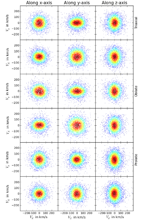
Figure 1: Velocity distributions inside three different locations of the Solar Neighborhood volumes: along the $x$-, $y$- and $z$-axis, obtained after integration for $8$ Gyr for the triaxial (top two rows), oblate (middle two rows), and prolate (bottom two rows) dark matter halo. In all cases is the major axis is aligned with the $z$-direction.

3.2 Kullback-Leibler Divergence

To quantify further whether there are any significant substructures in the velocity distributions, we apply the Kullback-Leibler Divergence (hereafter: KLD). The KLD is a statistic that measures the relative entropy or information content of two distributions, and can be used to determine the relative degree of clumpiness. We use the KLD to compare the velocity distribution $P(i,j,k)$ found for the particles in our simulations sampled on a three-dimensional cartesian grid in velocity space $(i,j,k)$ to a smooth velocity distribution $Q(i,j,k)$ computed on the same grid. For discrete probability distributions in three dimensions we define the KLD statistic $\alpha$ as:

$$\alpha=\sum_{i,j,k}P(i,j,k)\ln{\left(\frac{P(i,j,k)}{Q(i,j,k)}\right)}.$$ (6)

The larger the value of $\alpha$, the more clumpy the distribution. We use three different bin sizes, $25$ km/s, $50$ km/s, and $100$ km/s, loosely tuned to the size of the orbital structures (highlighted in the next Section). The total number of particles in the volume is typically $N_{tot}\sim 3000$.

The smooth velocity distribution used for comparison, $Q(i,jk)$, is obtained by randomly shuffling the velocity distribution found in the simulations. We couple each value of $v_{x}$ with a randomly selected $v_{y}$ and $v_{z}$ (without replacement). In this way, we generate 5,000 shuffled data sets and average the binned values to obtain $Q(i,j,k)$, making sure that any correlations and clumpiness are broken (see e.g. Sanderson et al., 2015)

To establish the statistical significance of a given value $\alpha$ found in our simulations, we determine how likely it is to obtain it in the shuffled data sets. We construct a distribution of $\alpha_{shuffle}$ by computing, for each of the 5,000 shuffled data sets, the $\alpha$ value using Equation (6). We may now calculate the probability $p_{shuffle}=N(\alpha_{shuffle}\geq\alpha_{sim})/N_{tot}$ of finding a value of $\alpha_{shuffle}$ as large as or larger than the measured $\alpha_{sim}$. To obtain more robust results, we have analysed the orbital integrations at 7 different outputs, starting from 8 Gyr up to 20 Gyr in total.

The vast majority of the volumes have median $p_{shuffle}>0.1$ for all potentials, whether axisymmetric or triaxial, demonstrating that on average, there are no significant differences in the amount of kinematic substructure present. Every now and then, a volume might depict a low value of $p_{shuffle}\sim 0.001$. This happens for the oblate and for the triaxial halos with similar frequency, indicating that, although the kinematic distribution might show some degree of lumpiness (on scales of 50 km/s), this is not necessarily a signature of triaxiality.

4 Orbital Analyses

4.1 Characterization of Orbital Resonances

Orbits that are quasi-periodic can be expressed as:

$$\@vec{q}(t)=\sum_{k=1}^{\infty}\@vec{a_{k}}e^{iF_{k}t}$$ (7)

where $\@vec{q}(t)$ is the vector of the spatial coordinates, $\@vec{a_{k}}$ the vector of the amplitudes, and the frequencies $F_{k}$ are linear combinations of $N_{b}$ base frequencies. Therefore the Fourier transform of a quasi-periodic orbit will consist of a sum of peaks with amplitudes $\@vec{a_{k}}$. In general, one is interested in determining the number and the numerical values of the base frequencies $\@vec{F_{b}}$. Orbits in a triaxial potential probe three-dimensional regions of space and therefore most will have three base-frequencies, $N_{b}=3$, unless the frequencies are commensurate, i.e. they are on a resonance. On the other hand, there may be orbits that are irregular and so cannot be described by Equation (7). In practise this might be taken to mean that the frequencies found by assuming Eq. (7) will be (combinations of) more than 3 frequencies, and hence these cannot be properly called base frequencies.

We apply the spectral orbit classifier of Carpintero & Aguilar (1998) to identify the base frequencies of the orbits in our simulations. After obtaining the time-series of the orbits through numerical integration, we identify the dominant frequencies $F_{d}$ by taking the frequencies with the highest amplitudes $a_{k}$. In all cases, we use the time-series in cartesian coordinates, i.e. $x$, $y$, and $z$. Accordingly, we find three groups of dominant frequencies $\@vec{F_{x,d}}$, $\@vec{F_{y,d}}$, and $\@vec{F_{z,d}}$ for each orbit where we consider a maximum of five per group. Through a process of subtracting the dominant frequencies and multiples thereof from the power spectra and reanalyzing the spectra, the orbit classifier of Carpintero & Aguilar (1998) determines the number $N_{b}$ of fundamental frequencies $F_{b}$ that describe the motion of each particle.

The so-called ‘frequency maps’ (Binney & Tremaine, 2008) are obtained by plotting $F_{2,b}/F_{3,b}$ versus $F_{1,b}/F_{3,b}$ help to visualize the structure in frequency space (e.g. Valluri et al., 2012, 2013). For regular orbits that are on a resonance we expect the base frequencies to be coupled in two or three dimensions. We define an orbital resonance when the ratios of the base frequencies in two or three dimensions is a rational number. This can be expressed by:

$$l_{1}F_{1,b}+l_{2}F_{2,b}+l_{3}F_{3,b}=0,$$ (8)

where $l_{1}$, $l_{2}$, and $l_{3}$ are integers and $F_{1,b}$, $F_{2,b}$, and $F_{3,b}$ are the base frequencies. Particles on orbital resonances therefore populate straight lines in the frequency map.

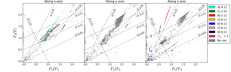
Figure 2: Frequency map for $\sim 3000$ particles located inside “Solar neighbourhood” spheres of radius $2$ kpc located on the $x$-, $y$-, and $z$-axes, obtained by orbital integration within the triaxial NFW. The orbital resonances can be distinguished by lines that follow the equation $l_{1}F_{1,b}+l_{2}F_{2,b}+l_{3}F_{3,b}=0$ with all $l$ integer numbers and $\@vec{F_{b}}$ the three base frequencies. The conditions are that particles are within a range of +/- 0.01 of a specific resonance line, at least ten particles populate the resonance, the integers $l$ of the resonance are all smaller than 10, and there is a distinct region around the line that is not populated. This last condition is partly violated in the case of resonance [6:4:1] on the $x$-axis, but we decided to include it for exploratory purposes.

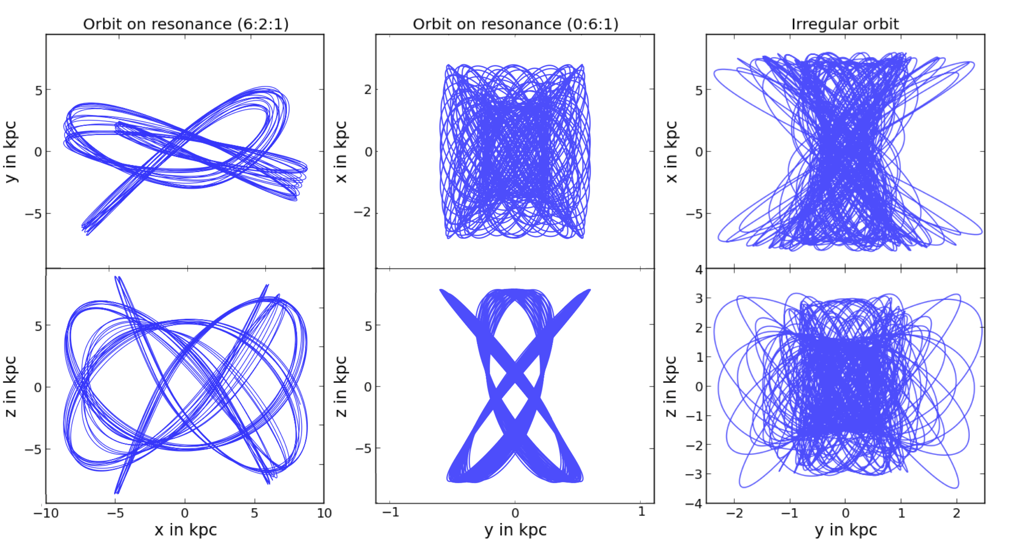
Figure 3: Examples of three orbits integrated in the triaxial NFW-potential for 15 Gyr. The left and middle panels correspond to orbits on the resonances [$l_{1}$:$l_{2}$:$l_{3}$] = [6:2:1] and [0:6:1] respectively, while the panel on the right shows an irregular orbit with $N_{b}>$ 3.

4.2 Resonance Populations Identified with Fourier Analysis

We analyze the orbits of the particles in the volumes shown in Figure 1 and integrated for $\sim$65 Gyr, using the orbit classifier of Carpintero & Aguilar (1998). In Figure 2 we plot the resulting frequency map $F_{1,b}/F_{3,b}$ versus $F_{2,b}/F_{3,b}$ for the triaxial potential. We use Equation (8) to identify the particles that populate resonances and the different types of resonances. This is done under a number of conditions, namely $i$) that particles are within a range of +/- 0.01 of a specific resonance line, $ii$) at least ten particles populate the resonance, $iii$) the integers $l$ of the resonance are all smaller than 10, and $iv$) there is a distinct region around the line that is not populated. These resonances are indicated with different colours in Fig. 2. It is evident from this figure that the orbital structure is different from volume to volume, and that the prominence of resonant orbits also varies with location.

We also use the orbit classifier of Carpintero & Aguilar (1998) to determine the fractions of orbits of different types (regular, resonant, irregular) in the various volumes. Figure 3 shows some examples of the types of orbits found in the triaxial potential. Table 1 summarizes the overall findings regarding the fractional distribution of the irregular orbits, non-resonant regular orbits, the resonant orbits (coupled in two or three dimensions), and the thin orbits (i.e., orbits for which the orbit classifier only found two base frequencies). On the major axis ($z$) in the triaxial potential $\sim$18% of the particles populate resonant orbits. More than half of these particles are on orbits that are coupled in three dimensions, they populate the resonances [$l_{1}$:$l_{2}$:$l_{3}$] = [6:2:1], [3:6:1], [2:8:1], and [6:8:1]. The remainder resonant orbits are coupled in only two dimensions. For the volumes on the intermediate and minor axes we see a much smaller fraction of resonant orbits ($\sim$2–4%). Note as well that in the volume on the major axis there is a much larger fraction of irregular orbits ($\sim$ 25%) compared to the intermediate and minor axes ($\sim$ 5%).

Similar analyses for two volumes $\sim$14 degrees off-axis from the major and minor axes showed orbital populations comparable to those found on the principal axes closest to these volumes.

The oblate and prolate potentials showed only resonances coupled in two dimensions. Again the volumes on the major axes show larger fractions of resonant orbits than those on the minor axes. The fraction of irregular orbits in the various volumes are generally much smaller in these potentials (oblate: $<$ 12%; prolate: $<$ 4%).

In summary, we note that in each volume the fractions of resonant orbits and irregular orbits are very small compared to the fraction of non-resonant regular orbits. Only on the major axis of the triaxial potential the fractions of both resonant and irregular orbits are higher (each contribute close to 20%). If present, the resonances are always of high order.

Table 1: The fractional distribution of non-resonant orbits (regular and irregular), resonant orbits (coupled in two or three dimensions) and thin orbits on the $x$-, $y$-, and $z$-axes in the triaxial NFW. The $x$-, $y$- and $z$-axes are aligned with the minor, intermediate, and major axes of the potential.

Triaxial		x	y	z
Non-resonant	Regular (%)	88.6	91.8	57.3
	Irregular (%)	6.6	4.1	23.1
Resonant	2D-coupled (%)	0.6	1.1	7.9
	3D-coupled (%)	3.5	0.9	10.1
Thin(%)		0.8	2.0	1.6

4.3 Resonance Populations in Velocity Space

Now we link the information of the resonance groups from Section 4.2 back to the velocity distributions of the particles for the selected Solar neighbourhood volumes. The resonant populations identified in frequency space are shown in Figure 4 with the same colour coding in velocity space for the triaxial potential. We see that for the volumes located on and near the major axis $z$ different resonances appear to populate different cylindrical shells in velocity space, all varying in their orientation. For example, the resonance [$l_{1}$:$l_{2}$:$l_{3}$] = [3:6:1] (in orange) forms a small well-defined “ring” at $|V_{x,y}|\sim 50$ km/s in the top right panel of Figure 4, while the resonance [6:2:1] (in red) forms two “walls” which have the range of +/- 150 km/s in $V_{x}$ and $V_{z}$ centered on $V_{y}$ = 50 km/s and $-50$ km/s. The particles on thin orbits populate mainly the regions of $|V_{y}|>100$ km/s. On the $x$- and $y$-axes much smaller fractions of the particles populate resonances and the patterns are not as pronounced as on the $z$-axis. Nevertheless, some features can be distinguished. For example, the resonance [6:8:1] forms a narrow line at $V_{x}=V_{z}=0$ km/s on the $y$-axis and particles from the resonance [6:4:1] mostly populate a bar-shaped region of thickness 50 km/s centered on $V_{z}$ = 0 km/s.

Similar behaviour is found for two volumes   14 degrees off-axis for the major and minor axes, as well as for the orbital integrations including a disk component, where regions in velocity space can be related to orbital resonances.

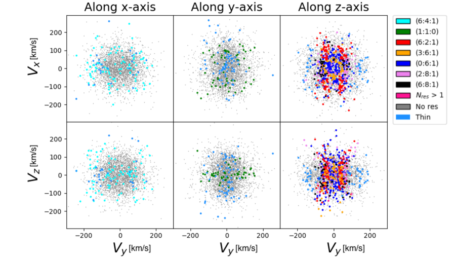
Figure 4: Velocity distributions inside the volumes along the $x$, $y$, and $z$-axes with the orbital resonances represented by different colors as in Fig. 2.

5 Discussion

The analysis presented above does not support the main claim of Rojas-Niño et al. (2012) that orbital resonances should be readily apparent in the velocities of nearby halo stars and therefore could be used for constraining the shape of the Milky Way’s dark matter halo. Although certain regions in the velocity distribution can indeed be related to resonances, we find in our model that the prominence of these features and the associated number of stars is very small. The reason for this disagreement can be explained by closer inspection of the methods used for setting up the orbital initial conditions.

In their set-up, Rojas-Niño et al. (2012) integrate the positions and velocities of stars initially located in a 1 kpc Solar-neighbourhood-like sphere, and focus on the kinematical structure in the same volume after 12 Gyr of evolution. This effectively pre-selects particles on resonant orbits, since those not associated to any resonance are less likely to return to the same volume on a relatively “short” timescale. This crucial difference explains why we find that the vast majority of orbits in such volumes are regular but non-resonant, and why we find smoother velocity distributions. To confirm this explanation we show in Figure 5 how the velocity distribution in our simulations would appear if we had pre-selected the particles on resonances coupled in three dimensions (i.e., most likely to return to the same volume). The resulting pattern is similar to that shown by Rojas-Niño et al. (2012) in their Fig. 3.

More recently Rojas-Niño et al. (2015) attempted to reduce this selection bias by increasing the volume of the sphere where the initial conditions were sampled. For example, the positions were generated uniformly within a 25 kpc radius sphere, and the velocities were sampled randomly between zero and the escape velocity at each location. This clearly implies a density distribution that does not fall off with radius, which is unlike that observed for stellar halos, and which presumably oversamples the outer regions of the velocity distribution, perhaps leading to an overpopulation of resonant orbits (see, e.g., Merritt & Valluri, 1999).

If the stellar halo was built via accretion (Helmi & White, 1999), the traces of these events are expected to be visible as substructures in velocity space (Helmi, 2008; Gómez et al., 2013). Depending on the infall parameters of these building blocks and on the gravitational potential of our Galaxy, the debris could be more evident if on resonant orbits (as argued by Rojas-Niño et al., 2012), or very difficult to detect if on chaotic orbits as the stars will drift away more quickly (Price-Whelan et al., 2015). First attempts to quantify the likelihood of this in a cosmological setting have been reported by Gómez et al. (2013); Maffione et al. (2015). In our simulations, the fractions of irregular orbits are only relatively large in the volumes located near the major axis of the triaxial potential. This could imply a bias in the accretion events that are amenable to recovery as substructures in velocity space. This is also relevant for the detection of streams in external galaxies, where those that may be more prone to detection may be those that are on specific resonant orbits. It will be important to quantify the likelihood of this and establish the resulting biases for constraining the accretion or merger history of a galaxy (but see, e.g. Maffione et al., 2018).

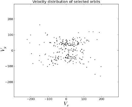
Figure 5: Velocity distribution of the particles located in a Solar Neighborhood volume of radius $1.5$ kpc at 8.5 kpc from the center on the $x$-axis after selecting only the particles that populate the resonances ($l_{1}$:$l_{2}$:$l_{3}$) = (6:2:1), (3:6:1), and (2:8:1). Although substructure is clearly apparent, most particles in this volume are on regular non-resonant orbits which yields velocity distributions as those shown in Fig. 4.

6 Conclusions

We have conducted numerical experiments with test particles in a Milky Way-like dark matter halo of three different shapes: triaxial, oblate, and prolate. To this end we generated initial conditions for these test particles following a smooth nearly self-consistent distribution function. The goal was to investigate the assertion of Rojas-Niño et al. (2012) that orbital resonances caused by the shape of the halo would leave imprints in the velocity space of Solar Neighborhood halo stars.

On the basis of the detailed analysis of the kinematics and orbital properties of particles located inside Solar neighbourhood volumes along the principal axes of the dark halo we have reached the following conclusions:

1. The shape of the velocity ellipsoid in these volumes is the only evident difference between experiments using triaxial, oblate, prolate, and spherical dark matter halos, whether including a disk component or not.

2. The velocity distributions within the Solar Neighborhood volumes do not show any significant substructures for either of the potentials explored, including the triaxial NFW with a disk component.

3. While resonances are indeed present and related to specific regions in velocity space, the fraction of particles associated to resonant orbits is small even for extreme values of the axis ratios that are still consistent with cosmological dark-matter-only simulations.

Our numerical experiments show that a smooth and more realistic initial distribution function does not favor any particular orbital resonance that can clearly differentiate among plausible shapes for the Galactic dark matter halo. We conclude that the most promising way to pin down its shape using the kinematics of halo stars would be to inspect the changes in the velocity ellipsoids across the Galaxy. This ought to be feasible with the six-dimensional phase-space information of stars that will soon be provided by the Gaia mission (Gaia Collaboration et al., 2016a, b).