Testing the Cosmic Shear Spatially-Flat Universe Approximation with Generalized Lensing and Shear Spectra

Abstract

We introduce the Generalised Lensing and Shear Spectra (GLaSS) code which is available for download from https://github.com/astro-informatics/GLaSS It is a fast and flexible public code, written in Python, that computes generalized spherical cosmic shear spectra. The commonly used tomographic and spherical Bessel lensing spectra come as built-in run-mode options. GLaSS is integrated into the Cosmosis modular cosmological pipeline package. We outline several computational choices that accelerate the computation of cosmic shear power spectra. Using GLaSS, we test whether the assumption that using the lensing and projection kernels for a spatially-flat universe – in a universe with a small amount of spatial curvature – negligibly impacts the lensing spectrum. We refer to this assumption as The Spatially-Flat Universe Approximation, that has been implicitly assumed in all cosmic shear studies to date. We confirm that The Spatially-Flat Universe Approximation has a negligible impact on Stage IV cosmic shear experiments.

I Introduction

The shape of distant galaxies is distorted by inhomogeneities in the gravitational field along the line of sight; a phenomenon known as gravitational lensing. When the distortion is small, as is most commonly the case, the change in shape is a change in the size and ellipticity of the observed image; known as shear. The gravitational lensing caused by large-scale structure, and in particular the two-point correlation function or power spectrum of this effect, is called cosmic shear.

Experiments that measure cosmic shear are sensitive to the physics of the late Universe, making them an ideal probe to distinguish between models of dark energy Refregier et al. (2010). Stage IV weak lensing experiments, that include Euclid Laureijs et al. (2010), WFIRST Spergel et al. (2015) and LSST Anthony and Collaboration , will provide an order of magnitude improvement in the precision and accuracy of cosmological parameter estimation over existing surveys Albrecht et al. (2006).

To prepare for these upcoming experiments we must prepare fast and accurate codes to compute the theoretical cosmic shear power spectra for any cosmology. While there are already publicly available tomographic lensing codes that use the Limber approximation Kilbinger et al. (2009); Zuntz et al. (2015), there are no other codes that can compute the cosmic shear power spectra with an arbitrary weight function. It remains an open question which weight-function optimally extracts cosmological information, and we leave this for a future work.

Also, before the arrival of Stage IV data, it is vital to test the validity of all assumptions used in cosmic shear studies. One of these approximations is that for the purposes of computing the cosmic shear power spectra we can always treat the Universe as spatially flat. This is an assumption that has not been tested previously.

The structure of this paper is as follows. In Section II we review the equations for the cosmic shear power spectra and the effect of spatial-curvature on the lensing kernel and projection kernel. In Section III we introduce GLaSS, which computes lensing spectra, and discuss a few computational choices that we implemented to speed up the computation of cosmic shear power spectra. Finally in Section IV we demonstrate the speed of GLaSS and discuss the impact of the Spatially-Flat Universe Approximation.

II Formalism

II.1 Generalized-Spherical Lensing Spectra

The generalized spherical-transform is defined in Taylor et al. (2018):

$$\gamma_{\ell m}\left(\eta\right)=\sqrt{\frac{2}{\pi}}\sum_{g}\gamma_{g}\left(r_{g},\boldsymbol{\theta_{g}}\right)W_{\ell}\left(\eta,r_{g}\right){}_{2}Y_{\ell m}\left(\boldsymbol{\theta_{g}}\right),$$ (1)

where $\gamma\in\mathbb{C}$ is the shear, the sum is over all galaxies $g$ with angular coordinate ${\bf\theta_{g}}$ and radial coordinate $r_{g}$, $W_{\ell}$ is a weight and ${}_{2}Y_{\ell m}$ are the spin-$2$ spherical harmonics. The cosmic shear power spectrum in this basis is:

$$C_{\ell}^{\gamma\gamma}\left(\eta_{1},\eta_{2}\right)=\frac{9\Omega_{m}^{2}H_{0}^{4}}{16\pi^{4}c^{4}}\frac{\left(\ell+2\right)!}{\left(\ell-2\right)!}\int\frac{\text{d}k}{{k}^{2}}G_{\ell}^{\gamma}\left(\eta_{1},k\right)G_{\ell}^{\gamma}\left(\eta_{2},k\right),$$ (2)

where $\Omega_{m}$ is the fractional energy density of matter, $c$ is the speed of light in vacuum and $H_{0}$ is the value of the Hubble constant today. The $G$-matrix is:

$$G_{\ell}^{\gamma}\left(\eta,k\right)\equiv\int\text{d}z_{p}\text{d}z^{\prime}\text{ } n\left(z_{p}\right)p\left(z^{\prime}|z_{p}\right)$$ (3)

$$\times W_{\ell}\left(\eta,r\left[z^{\prime}\right]\right)U_{\ell}\left(r\left[z^{\prime}\right],k\right)$$

where $r[z]$ is the co-moving distance at a redshift $z$ and the $U$-matrix is:

$$U_{\ell}\left(r[z],k\right)\equiv\int^{r}_{0}\text{d}r^{\prime}\text{ }\frac{F_{K}\left(r,r^{\prime}\right)}{a\left(r^{\prime}\right)}j_{\ell}\left(kr^{\prime}\right)P^{1/2}\left(k;r^{\prime}\right),$$ (4)

where $a$ is the scale factor, $j_{\ell}(kr)$ are the spherical Bessel functions and $P(k;r)$ is the power spectrum. The radial distribution of galaxies is denoted by $n(z)$ and $p\left(z|z^{\prime}\right)$ gives the probability that a galaxy has a redshift $z$, given a photometric redshift measurement $z^{\prime}$. For a spatially-flat cosmology the lensing kernel, $F_{K}\left(r,r^{\prime}\right)$, is:

$$F_{K}\left(r,r^{\prime}\right)\equiv\frac{r-r^{\prime}}{rr^{\prime}}.$$ (5)

The power spectrum caused by the random ellipticity component of galaxies, the shot noise spectrum, is given by:

$$N_{\ell}^{ee}\left(\eta_{1},\eta_{2}\right)=\frac{\sigma_{e}^{2}}{2\pi^{2}}\int\text{d}z\text{ }n\left(z\right)W_{\ell}\left(\eta_{1},r\right)W_{\ell}\left(\eta_{2},r\right),$$ (6)

where $\sigma_{e}^{2}$ is the variance of the intrinsic (unlensed) ellipticities of the observed galaxies. We take $\sigma_{e}=0.3$ throughout Brown et al. (2003).

Taking the weight-function, $W_{\ell}\left(\eta,r\left[z\right]\right)\equiv j_{\ell}\left(\eta r[z]\right)$ in equations (3) and (6) yields the equations for ‘3D cosmic shear’ first proposed in Heavens (2003). To recover the ‘tomographic’ cosmic shear spectra, first proposed in Hu (1999), we take the weight function, $W^{I}$, as a top hat function in redshift only:

$$W^{I}\left(z\right)\equiv\begin{cases}1&\text{if $z\in I$ }\\ 0&\text{if $z\notin I$, }\\ \end{cases}$$ (7)

the tomographic bin associated with redshift region $I$.

Taking the Limber approximation  LoVerde and Afshordi (2008), the $U$-matrix becomes:

$$U_{\ell}\left(r,k\right)=\frac{F_{k}\left(r,\nu\left(k\right)\right)}{ka\left(\nu\left(k\right)\right)}\sqrt{\frac{\pi}{2\left({\ell}+1/2\right)}}P^{1/2}\left(k,\nu\left(k\right)\right),$$ (8)

where $\nu\left(k\right)\equiv\frac{{\ell}+1/2}{k}$. This is a good approximation for $\ell>100$ Kitching et al. (2016); Kilbinger et al. (2017).

II.2 The Lensing Kernel for $\Omega_{k}\neq 0$

In a spatially-curved universe, the expression for the lensing kernel in equation (5) must be replaced by the more general expression:

$$F_{K}\left(r,r^{\prime}\right)\equiv\frac{f_{k}\left(r-r^{\prime}\right)}{f_{k}\left(r\right)f_{k}\left(r^{\prime}\right)},$$ (9)

where $f_{k}(r)$ is the co-moving angular distance Kilbinger (2015). This is given by:

$$f_{K}\left(r\right)\equiv\begin{cases}K^{-1/2}\text{sin}\left(K^{1/2}r\right)&\text{if $K>0$ }\\ r&\text{if $K=0$. }\\ \left(-K\right)^{-1/2}\text{sinh}\left(\left(-K\right)^{1/2}r\right)&\text{if $K<0$. }\\ \end{cases}$$ (10)

where the curvature, $K$, is defined as $K\equiv-\left(H_{0}/c\right)^{2}\Omega_{k}$, and $\Omega_{k}$ is the spatial curvature density today.

II.3 The Projection Kernel for $\Omega_{k}\neq 0$

In a spatially-flat universe, the gravitational potential at a time labeled by the redshift $z$, $\Phi\left({\bf r};z\right)$, is related to the underlying density field, $\delta\left({\bf r};z\right)$, by the Poisson equation:

$$\nabla_{r}^{2}\Phi\left({\bf r};z\right)=\frac{3\Omega_{m}H_{0}^{2}}{2a\left(t\right)}\delta\left({\bf r};z\right),$$ (11)

where $\nabla^{2}_{r}$ is the Laplacian associated with a spatially-flat universe.

The potential, $\Phi\left({\bf r};z\right)$, in the observer’s frame is given in a coordinate system defined by two angles on the sky and a radial distance denoted by $(r,\theta,\phi)$. Meanwhile the density field is in rectilinear coordinates. To relate the two, and hence find the lensing spectra in terms of the matter power spectrum, we expand the potential in spherical Bessel space:

$$\Phi_{\ell m}\left(k\right)=\sqrt{\frac{2}{\pi}}\int\text{d}^{3}r\text{ }\Phi\left(r\right)j_{\ell}\left(kr\right)Y_{\ell m}\left(\theta,\phi\right),$$ (12)

where $j_{\ell}\left(kr\right)$ are spherical Bessel functions and $Y_{\ell m}\left(\theta,\phi\right)$ are spherical harmonics. Then since spherical harmonics and spherical Bessel functions are eigenfunctions of the Laplace operator, we have:

$$\left(\nabla_{r}^{2}+k^{2}\right)j_{\ell}\left(kr\right)Y_{\ell m}\left(\theta,\phi\right)=0,$$ (13)

and from equation (11) the lensing potential is related to the density field in harmonic space by:

$$\Phi_{\ell m}\left(k;z\right)=-\frac{3\Omega_{m}H_{0}^{2}}{2k^{2}a\left(t\right)}\delta_{\ell m}\left(k;z\right).$$ (14)

From this it is possible to derive the expression for the cosmic shear power spectrum. Since Bessel functions relate the lensing potential in rectilinear coordinates to a projected shear signal on the sky, we refer to $j_{\ell}\left(kr\right)$ as the projection kernel. In the final expression for the cosmic shear power spectra, the projection kernel is found in the $U$-matrix (see Castro et al. (2005) for a full derivation).

Meanwhile in a spatially-curved universe, we must take the Laplacian associated with the curved Robertson-Walker metric Kosowsky (1998) in equation (11). Hence the projection kernel must change too. In particular spherical Bessel functions must be replaced by hyperspherical Bessel functions, $\Phi^{\beta}_{l}\left(r\right)$, because they are eigenfunctions of the the Laplace operator in a spatially-curved cosmology. That is:

$$\left(\nabla_{S_{K}(\chi)}^{2}+(ck)^{2}\right)\Phi^{\beta}_{\ell}\left(\chi\right)Y_{\ell m}\left(\theta,\phi\right)=0,$$ (15)

where $\beta\equiv\sqrt{(ck)^{2}+K}$, $\chi=r/c$ and

$$S_{K}\left(\chi\right)\equiv\begin{cases}\sin{\chi}&\text{if $K>0$ }\\ \chi&\text{if $K=0$ }\\ \sinh{\chi}&\text{if $K<0$. }\\ \end{cases}$$ (16)

Following the same argument used in the spatially-flat case, we find the hyperspherical Bessel functions enter the $U$-matrix, in place of the normal spherical Bessel functions, as the projection kernel.

The Limber approximation also has to be generalized to spatially-curved cosmologies Lesgourgues and Tram (2014). In this case the Limber-approximated $U$-matrix becomes:

$$U_{\ell}\left(r,k\right)=\left(1-\hat{K}\frac{\ell^{2}}{\beta^{2}}\right)^{-\frac{1}{4}}U^{\rm flat}_{\ell}\left(r,k\right),$$ (17)

where $\hat{K}$ is the sign of the curvature $K$, and $U^{\rm flat}_{\ell}\left(r,k\right)$ is the Limber approximated $U$-matrix for a spatially-flat universe defined in equation (8).

III The GLaSS Code

We now describe the GLaSS code that can compute all the power spectra previously described.

III.1 Description and Run Options

GLaSS is a flexible code written in Python and it is fully integrated into the Cosmosis modular cosmological pipeline Zuntz et al. (2015). The code is provided with Python wrappers and cosmological information can be read directly from the Cosmosis pipeline or from an external source.

There are numerous run-mode options. The user can choose between several weights. These include: the top hats associated with tomographic binning with an equal number of galaxies per bin or equally spaced tomographic bins in redshift, the spherical Bessel weight, or a customized weight provided by the user. The number of tomographic bins can also be varied. The user can specify which $\ell$-modes to sample over a prescribed redshift range. The package is distributed with default functional forms for the radial distribution of galaxies, $n(z)$, and photometric redshift error $p\left(z|z^{\prime}\right)$. These are:

$$p\left(z|z_{p}\right)\equiv\frac{1}{2\pi\sigma_{z}\left(z_{p}\right)}e^{-\frac{\left(z-c_{\rm cal}z_{p}+z_{\rm bias}\right)^{2}}{2\sigma_{z_{p}}}},$$ (18)

with $c_{\rm cal}=1$, $z_{\rm bias}=0$ and $\sigma_{z_{p}}=A\left(1+z_{p}\right)$, with default value is $A=0.05$ Ilbert et al. (2006) and

$$n\left(z_{p}\right)\propto\frac{a_{1}}{c_{1}}e^{-\frac{\left(z-0.7\right)^{2}}{b_{1}^{2}}}+e^{-\frac{\left(z-1.2\right)^{2}}{d_{1}^{2}}},$$ (19)

with default values $\left(a_{1}/c_{1},b_{1},d_{1}\right)=\left(1.5/0.2,0.32,0.46\right)$ Van Waerbeke et al. (2013). It is possible for the user to provide custom functional forms too.

The Limber approximation can be turned on or off. Since the Limber approximation is less accurate at low-$\ell$ Kitching et al. (2016), it can be turned on for any chosen $\ell>\ell_{\rm Lim}$, for a specified value of $\ell_{\rm Lim}$.

Finally it is possible to independently turn the spatially-curved lensing kernel and projection kernel approximations on or off; however later we show these approximations have negligible impact. Hyperspherical Bessel functions are computed with a Python wrapper that calls CLASS Blas et al. (2011). Details about the implementation of the hyperspherical Bessel functions in CLASS are given in (Tram (2017) and Lesgourgues and Tram (2014)).

GLaSS has been compared to the spherical Bessel code used in Spurio Mancini et al. (2018) and gives very similar output when using the spherical Bessel weight (Spurio Mancini et al. in prep).

III.2 Computational Choices

Several numerical choices have been implemented in GLaSS to reduce the computation time.

Values of the Bessel functions, $j_{\ell}\left(x\right)$, are computed just once and stored in a 2D look up table in $\ell$ and $x$. The values of $j_{\ell}\left(kr\right)$, can then be found as needed. We sample sufficiently densely in $x$ so that final lensing spectra is not affected above machine precision. Compressing the data in this way reduces memory requirements and was used before in Seljak and Zaldarriaga ; Kosowsky (1998). In the hyperspherical case, it is not possible to compress the data to a 2D-array. In this case the hyperspherical Bessel functions are computed on the fly, slowing down the total computation time.

Even though the Bessel functions need only be computed once, the computation of these has also been optimized in GLaSS. For a given argument $x$, GLaSS computes and stores all $j_{\ell}(x)$ for all $\ell$-modes simultaneously using Miller’s algorithm which is based on recurrence relations and implemented in the GNU Scientific Library Gough (2009), and called using ctypesGSL. If the maximum $\ell$ is too high, Miller’s algorithm suffers from underflow. GLaSS avoids this by first sparsely sampling the $x$-range to determine a maximum $\ell_{\text{max}}\left(x\right)$, for each $x$, which is defined as the $\ell$-value past which the Bessel functions fall below machine precision. GLaSS sets $j_{\ell}(x)=0$ for all $\ell>\ell_{\text{max}}\left(x\right)$.

As the Bessel functions are pre-computed, the majority of the computation time is taken by evaluating the nested integrals in equations (1) - (4). In GLaSS all these are evaluated using matrix multiplications on a grid in $r$ and $k$. For example the $U$-matrix can be written as a matrix multiplication given by:

$$U_{\ell}\left(r,k\right)\approx\sum_{r^{\prime}}A\left(r,r^{\prime}\right)B\left(r^{\prime},k\right),$$ (20)

$A\left(r,r^{\prime}\right)\equiv\Delta r^{\prime}\frac{F_{K}\left(r,r^{\prime}\right)}{a\left(r^{\prime}\right)}$, where $\Delta r^{\prime}$ is the spacing of the grid in $r^{\prime}$ and $B\left(r,r^{\prime}\right)\equiv j_{\ell}\left(kr^{\prime}\right)P^{1/2}\left(k;r^{\prime}\right).$

All matrix multiplications in GLaSS are implemented using the numpy.dot function. This is one of the few functions that releases the Global Interpreter Lock in Python, so the matrix multiplications are parallelized when numpy is linked to a linear algebra library such as BLAS (Basic Linear Algebra Subprograms), Math Kernel Library (MKL) or Apple Accelerate. There are also MPI run-mode options for the Monte Carlo samplers in Cosmosis, which can be used to further distribute the workload over multiple cores.

The final speed improvements come from making the Limber approximation. Since the Bessel functions oscillate quickly, particularly for high-$\ell$, making the Limber approximation reduces the size of the computation grid needed to accurately evaluate the $U$-matrix. Meanwhile GLaSS can simultaneously turn the Limber approximation off at low-$\ell$ so that accuracy is not lost at these large angular scales where the Limber approximation is invalid.

IV Results

We now present results on the GLaSS computational scaling, and the impact of the spatially-flat universe approximation. In what follows we assume a 15,000 square degrees survey with 30 galaxies per $\text{arcmin}^{2}$ as predicted for the Euclid wide-field survey.

IV.1 GLaSS Module Timing

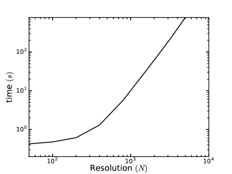
Figure 1: Time to compute $50$ $\ell$-modes in GLaSS against grid resolution $N$ (i.e. number of tomographic bins, or $k$-modes in 3D cosmic shear) on a single 2.7 GHz Intel i5 Core. Spectra for resolutions up to $N=400$ can all be computed in less than $1.5s$. This is a sufficient resolution to evaluate the tomographic cosmic shear power spectra and recover all information from the 3D shear field Taylor et al. (2018). At high-$\ell$, the computation time, $t$, is dominated by the matrix multiplications and hence scales as $t\propto N^{2.87}.$

We now present the results of several speed tests using GLaSS. All results cited are for $10$-bin tomography with an equal number of galaxies per bin sampling $50$ $\ell$-modes below $\ell_{\text{max}}=3000$ on a single 2.7 GHz Intel i5 Core on a 2015 Macbook Pro with $8$ GB of RAM.

It takes 28 seconds to compute all the Bessel function data, but this must only ever be computed once. This shows how vital it is to pre-compute the Bessel data.

The nested integral and hence the lensing spectra are computed on an $N\times N$ grid, where $N$ is the number of linearly sampled points in $z$ and logarithmically sampled points in $k$. For $N<300$, it takes less than a second to compute the lensing spectra when the Limber approximation is assumed for $\ell>100$.

As the resolution is increased beyond $N=600$, the computation time, $t$, follows the power law $t\propto N^{2.87}.$ This reflects the fact that the computation time becomes dominated by the nested matrix multiplications. Naively matrix multiplications scale as ${\mathcal{O}}\left(N^{3}\right)$ because all $N^{2}$ elements of the first matrix must be multiplied by $N$ elements in the second matrix. Our code does slightly better and scales as ${\mathcal{O}}\left(N^{2.87}\right)$ because it uses the highly optimized numpy.dot routine.

It was shown in Taylor et al. (2018) that a resolution of $N=400$ is sufficient to capture nearly all the lensing kernel and power spectrum information. Meanwhile a resolution of $N=2000$ is required to capture $80\%$ of the information when using the spherical Bessel weight and an extremely high resolution of $N=5000$ is needed to capture $97\%$ of the information for this choice of weight Taylor et al. (2018).

IV.2 Impact of the Flat Universe Approximation on Lensing Spectra

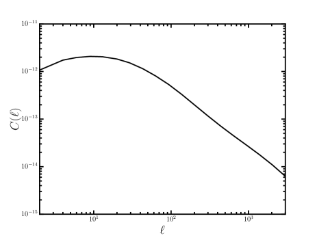
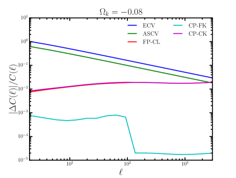
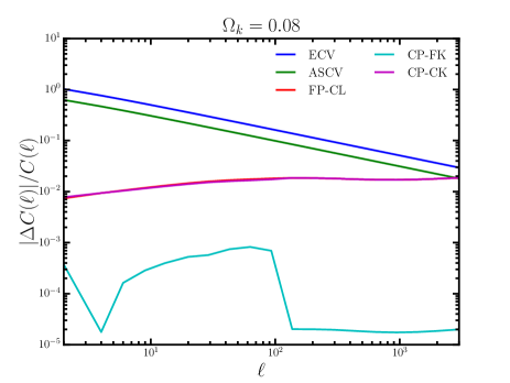
Figure 2: Top: The cross-correlated lensing spectrum, $C_{\ell}$, between tomographic bins $9$ and $10$, using the spatially-flat kernels. Middle: Relative change in $C_{\ell}$ for different kernels with $\Omega_{k}=-0.08$. The fiducial spectrum, $C_{\ell}$, uses the spatially-flat kernels. CP, FP, CL and FL respectively denote when the spatially-curved projection kernel, spatially-flat projection kernel, spatially-curved lensing kernel and spatially-curved lensing kernel, are used. The sample variance for Euclid-like (ECV) and the cosmic variance for a theoretical all sky survey (ASCV) are also shown. The relative change in $C_{\ell}$ is smaller than the sample variance for a Euclid-like survey for all $\ell<3000$. Bottom: Same as the middle figure, but with $\Omega_{k}=0.08$.

We compute the cosmic shear power spectra for a flat fiducial cosmology with: $\left(\Omega_{m},\Omega_{k},\Omega_{b},h_{0},n_{s},A_{s},\tau\right)=\left(0.315,\text{ }0.0,\text{ }0.04,\text{ }0.67,\text{ }0.96,\text{ }2.1\times 10^{9},\text{ }0.08\right)$. The linear power spectrum is generated using CAMB Lewis and Challinor (2011) and the non-linear part is generated using HALOFIT Takahashi et al. (2012). The Limber approximation is assumed for $\ell>100.$ The resulting cross-correlated lensing power spectrum between the highest redshift bins is shown at the top of Figure 2.

For $|\Omega_{k}|=0.08$, which is the expected $1\sigma$ constrain for a Euclid-like experiment Heavens et al. (2006), we have computed the lensing spectra inside the same bin using spatially-flat lensing and projection kernels (FP-FL). The same lensing spectra using: a spatially-curved projection kernel and spatially -flat lensing kernel (CP-FL), spatially-flat projection kernel and spatially-curved lensing kernel (FP-CL) and spatially-curved projection and lensing kernels (CP-CL) are computed. The relative difference, $\Delta C\left(\ell\right)/C\left(\ell\right)$, between the FP-FL spectrum and the others is shown in the bottom two panels of Figure 2. When the spatially-curved projection kernel is used, we employ the modified Limber approximation defined in (17) for $\ell>100$.

The sample variance for a Euclid-like survey is also shown in Figure 2 and is given by:

$$\Delta C\left(\ell\right)/C\left(\ell\right)=\sqrt{2}\left[f_{sky}\left(2\ell+1\right)\right]^{-1/2},$$ (21)

where $f_{sky}$ is the fraction of the sky observed by the survey Weinberg (2008).

In all cases we find that the relative difference between the spectra computed using the spatially-flat projection and lensing kernels are smaller than the sample variance, up to $\ell=3000$. This is true for the cross-correlation between all tomographic bins. Since the majority of the information from upcoming cosmic shear studies will be extracted from $\ell$-modes below $\ell=3000$Taylor et al. (2018), and the impact of changing the projection and lensing kernel is sub-dominant to the sample variance at these scales, it is safe to make the Spatially-Flat Universe Approximation for stage IV experiments.

Testing the impact of the Spatially-Flat Universe approximation with $|\Omega_{k}|=0.08$ was an extremely conservative choice. The 2015 Planck $2\sigma$ multi-probe constrain place $\left|\Omega_{k}\right|<0.005$ Ade et al. (2016). We have computed the impact of the Spatially-flat Universe Approximation in this case with $\left|\Omega_{k}\right|=0.005$ and found that relative difference, $\Delta C\left(\ell\right)/C\left(\ell\right)$, between the CP-CL and FP-FL falls a further order of magnitude from the $|\Omega_{k}|=0.08$ case shown in Figure 2.

V Conclusion

We have presented the GLaSS code that computes generalized cosmic shear power spectra. Spherical Bessel and tomographic lensing spectra with an equal number of galaxies per bin and equal redshift run-mode options are available. More generally GLaSS is capable of computing the lensing spectra with any data weighting. This should prove useful for determining the optimal weight for shear data in upcoming surveys.

GLaSS is fast. Using the Limber approximation, GLaSS can compute a $10$-bin tomographic lensing spectra for a single cosmology, sampling $50$ $\ell$-modes, in less than $0.4s$. For Stage IV experiments where the Limber approximation must be dropped below $\ell<100$, the same spectra is computed in $1.3s$.

Using GLaSS we have tested the Spatially-Flat Universe Approximation, which is implicitly assumed in all cosmic shear studies to date. We find this is an accurate approximation and it is unnecessary to compute the full expression for upcoming surveys.

References

- Refregier et al. (2010) A. Refregier, A. Amara, T. Kitching, A. Rassat, R. Scaramella, J. Weller, et al., arXiv preprint arXiv:1001.0061 (2010).
- Laureijs et al. (2010) R. J. Laureijs, L. Duvet, I. E. Sanz, P. Gondoin, D. H. Lumb, T. Oosterbroek, and G. S. Criado, in Proc. SPIE, Vol. 7731 (2010) p. 77311H.
- Spergel et al. (2015) D. Spergel, N. Gehrels, C. Baltay, D. Bennett, J. Breckinridge, M. Donahue, A. Dressler, B. Gaudi, T. Greene, O. Guyon, et al., arXiv preprint arXiv:1503.03757 (2015).
- (4) J. Anthony and L. Collaboration, in Proc. of SPIE Vol, Vol. 4836, p. 11.
- Albrecht et al. (2006) A. Albrecht, G. Bernstein, R. Cahn, W. L. Freedman, J. Hewitt, W. Hu, J. Huth, M. Kamionkowski, E. W. Kolb, L. Knox, et al., arXiv preprint astro-ph/0609591 (2006).
- Kilbinger et al. (2009) M. Kilbinger, K. Benabed, J. Guy, P. Astier, I. Tereno, L. Fu, D. Wraith, J. Coupon, Y. Mellier, C. Balland, et al., Astronomy & Astrophysics 497, 677 (2009).
- Zuntz et al. (2015) J. Zuntz, M. Paterno, E. Jennings, D. Rudd, A. Manzotti, S. Dodelson, S. Bridle, S. Sehrish, and J. Kowalkowski, Astronomy and Computing 12, 45 (2015).
- Taylor et al. (2018) P. L. Taylor, T. D. Kitching, and J. D. McEwen, arXiv preprint arXiv:1804.03667 (2018).
- Brown et al. (2003) M. L. Brown, A. N. Taylor, D. J. Bacon, M. E. Gray, S. Dye, K. Meisenheimer, and C. Wolf, Monthly Notices of the Royal Astronomical Society 341, 100 (2003).
- Heavens (2003) A. Heavens, Monthly Notices of the Royal Astronomical Society 343, 1327 (2003).
- Hu (1999) W. Hu, The Astrophysical Journal Letters 522, L21 (1999).
- LoVerde and Afshordi (2008) M. LoVerde and N. Afshordi, Physical Review D 78, 123506 (2008).
- Kitching et al. (2016) T. D. Kitching, J. Alsing, A. F. Heavens, R. Jimenez, J. D. McEwen, and L. Verde, arXiv preprint arXiv:1611.04954 (2016).
- Kilbinger et al. (2017) M. Kilbinger, C. Heymans, M. Asgari, S. Joudaki, P. Schneider, P. Simon, L. Van Waerbeke, J. Harnois-Déraps, H. Hildebrandt, F. Köhlinger, et al., Monthly Notices of the Royal Astronomical Society 472, 2126 (2017).
- Kilbinger (2015) M. Kilbinger, Reports on Progress in Physics 78, 086901 (2015).
- Castro et al. (2005) P. Castro, A. Heavens, and T. Kitching, Physical Review D 72, 023516 (2005).
- Kosowsky (1998) A. Kosowsky, arXiv preprint astro-ph/9805173 (1998).
- Lesgourgues and Tram (2014) J. Lesgourgues and T. Tram, Journal of Cosmology and Astroparticle Physics 2014, 032 (2014).
- Ilbert et al. (2006) O. Ilbert, S. Arnouts, H. McCracken, M. Bolzonella, E. Bertin, O. Le Fevre, Y. Mellier, G. Zamorani, R. Pello, A. Iovino, et al., Astronomy & Astrophysics 457, 841 (2006).
- Van Waerbeke et al. (2013) L. Van Waerbeke, J. Benjamin, T. Erben, C. Heymans, H. Hildebrandt, H. Hoekstra, T. D. Kitching, Y. Mellier, L. Miller, J. Coupon, et al., Monthly Notices of the Royal Astronomical Society 433, 3373 (2013).
- Blas et al. (2011) D. Blas, J. Lesgourgues, and T. Tram, Journal of Cosmology and Astroparticle Physics 2011, 034 (2011).
- Tram (2017) T. Tram, Communications in Computational Physics 22, 852 (2017).
- Spurio Mancini et al. (2018) A. Spurio Mancini, R. Reischke, V. Pettorino, B. M. Scháefer, and M. Zumalacárregui, arXiv preprint arXiv:1801.04251 (2018).
- (24) U. Seljak and M. Zaldarriaga, ApJ 469, 437.
- Gough (2009) B. Gough, GNU scientific library reference manual (Network Theory Ltd., 2009).
- Lewis and Challinor (2011) A. Lewis and A. Challinor, Astrophysics Source Code Library (2011).
- Takahashi et al. (2012) R. Takahashi, M. Sato, T. Nishimichi, A. Taruya, and M. Oguri, The Astrophysical Journal 761, 152 (2012).
- Heavens et al. (2006) A. Heavens, T. D. Kitching, and A. Taylor, Monthly Notices of the Royal Astronomical Society 373, 105 (2006).
- Weinberg (2008) S. Weinberg, Cosmology (Oxford University Press, 2008).
- Ade et al. (2016) P. Ade, N. Aghanim, M. Arnaud, M. Ashdown, J. Aumont, C. Baccigalupi, A. Banday, R. Barreiro, J. Bartlett, N. Bartolo, et al., Astronomy & Astrophysics 594, A13 (2016).