Approximating Operator Norms via Generalized Krivine Rounding

Abstract

We consider the $(\ell_{p},\ell_{r})$-Grothendieck problem, which seeks to maximize the bilinear form $y^{T}Ax$ for an input matrix $A\in{\mathbb{R}}^{m\times n}$ over vectors $x,y$ with $\|x\|_{p}=\|y\|_{r}=1$. The problem is equivalent to computing the $p\rightarrow r^{\ast}$ operator norm of $A$, where $\ell_{r^{*}}$ is the dual norm to $\ell_{r}$. The case $p=r=\infty$ corresponds to the classical Grothendieck problem. Our main result is an algorithm for arbitrary $p,r\geq 2$ with approximation ratio $(1+\varepsilon_{0})/(\sinh^{-1}(1)\cdot\gamma_{p^{\ast}}\,\gamma_{r^{\ast}})$ for some fixed $\varepsilon_{0}\leq 0.00863$. Here $\gamma_{t}$ denotes the $t$’th norm of the standard Gaussian. Comparing this with Krivine’s approximation ratio $(\pi/2)/\sinh^{-1}(1)$ for the original Grothendieck problem, our guarantee is off from the best known hardness factor of $(\gamma_{p^{\ast}}\gamma_{r^{\ast}})^{-1}$ for the problem by a factor similar to Krivine’s defect (up to the constant $(1+\varepsilon_{0})$).

Our approximation follows by bounding the value of the natural vector relaxation for the problem which is convex when $p,r\geq 2$. We give a generalization of random hyperplane rounding using Hölder-duals of Gaussian projections rather than taking the sign. We relate the performance of this rounding to certain hypergeometric functions, which prescribe necessary transformations to the vector solution before the rounding is applied. Unlike Krivine’s Rounding where the relevant hypergeometric function was $\arcsin$, we have to study a family of hypergeometric functions. The bulk of our technical work then involves methods from complex analysis to gain detailed information about the Taylor series coefficients of the inverses of these hypergeometric functions, which then dictate our approximation factor.

Our result also implies improved bounds for “factorization through $\ell_{2}^{n}$” of operators from $\ell_{p}^{n}$ to $\ell_{q}^{m}$ (when $p\geq 2\geq q$), and our work provides modest supplementary evidence for an intriguing parallel between factorizability, and constant-factor approximability.

1 Introduction

We consider the problem of finding the $p{\rightarrow}q$ norm of a given matrix $A\in{\mathbb{R}}^{m\times n}$, which is defined as

$$\mathchoice{\lVert A\rVert_{p\rightarrow q}}{\lVert A\rVert_{p\rightarrow q}}{\lVert A\rVert_{p\rightarrow q}}{\lVert A\rVert_{p\rightarrow q}}~{}:=~{}\max_{x\in{\mathbb{R}}^{n}\setminus\{0\}}\frac{\mathchoice{\lVert Ax\rVert_{q}}{\lVert Ax\rVert_{q}}{\lVert Ax\rVert_{q}}{\lVert Ax\rVert_{q}}}{\mathchoice{\lVert x\rVert_{p}}{\lVert x\rVert_{p}}{\lVert x\rVert_{p}}{\lVert x\rVert_{p}}}\,.$$

The quantity $\mathchoice{\lVert A\rVert_{p\rightarrow q}}{\lVert A\rVert_{p\rightarrow q}}{\lVert A\rVert_{p\rightarrow q}}{\lVert A\rVert_{p\rightarrow q}}$ is a natural generalization of the well-studied spectral norm ($p=q=2$) and computes the maximum distortion (stretch) of the operator $A$ from the normed space $\ell_{p}^{n}$ to $\ell_{q}^{m}$. The case when $p=\infty$ and $q=1$ is the well known Grothendieck problem [KN12, Pis12], where the goal is to maximize $\left\langle y,Ax\right\rangle$ subject to $\mathchoice{\lVert y\rVert_{\infty}}{\lVert y\rVert_{\infty}}{\lVert y\rVert_{\infty}}{\lVert y\rVert_{\infty}},\mathchoice{\lVert x\rVert_{\infty}}{\lVert x\rVert_{\infty}}{\lVert x\rVert_{\infty}}{\lVert x\rVert_{\infty}}\leq 1$. In fact, via simple duality arguments, the general problem computing $\mathchoice{\lVert A\rVert_{p\rightarrow q}}{\lVert A\rVert_{p\rightarrow q}}{\lVert A\rVert_{p\rightarrow q}}{\lVert A\rVert_{p\rightarrow q}}$ can be seen to be equivalent to the following variant of the Grothendieck problem

$$\mathchoice{\lVert A\rVert_{p\rightarrow q}}{\lVert A\rVert_{p\rightarrow q}}{\lVert A\rVert_{p\rightarrow q}}{\lVert A\rVert_{p\rightarrow q}}~{}=~{}\max_{\begin{subarray}{c}\mathchoice{\lVert x\rVert_{p}}{\lVert x\rVert_{p}}{\lVert x\rVert_{p}}{\lVert x\rVert_{p}}\leq 1\\ \mathchoice{\lVert y\rVert_{q^{*}}}{\lVert y\rVert_{q^{*}}}{\lVert y\rVert_{q^{*}}}{\lVert y\rVert_{q^{*}}}\leq 1\end{subarray}}\left\langle y,Ax\right\rangle~{}=~{}\mathchoice{\lVert A^{T}\rVert_{q^{*}\rightarrow p^{*}}}{\lVert A^{T}\rVert_{q^{*}\rightarrow p^{*}}}{\lVert A^{T}\rVert_{q^{*}\rightarrow p^{*}}}{\lVert A^{T}\rVert_{q^{*}\rightarrow p^{*}}}\,,$$

where $p^{*},q^{*}$ denote the dual norms of $p$ and $q$, satisfying $1/p+1/p^{*}=1/q+1/q^{*}=1$. The above quantity is also known as the injective tensor norm of $A$ where $A$ is interpreted as an element of the space $\ell_{q}^{m}\otimes\ell_{p^{*}}^{n}$.

In this work, we consider the case of $p\geq q$, where the problem is known to admit good approximations when $2\in[q,p]$, and is hard otherwise. Determining the right constants in these approximations when $2\in[q,p]$ has been of considerable interest in the analysis and optimization community.

For the case of $\infty{\rightarrow}1$ norm, Grothendieck’s theorem [Gro56] shows that the integrality gap of a semidefinite programming (SDP) relaxation is bounded by a constant, and the (unknown) optimal value is now called the Grothendieck constant $K_{G}$. Krivine [Kri77] proved an upper bound of $\pi/(2\ln(1+\sqrt{2}))=1.782\ldots$ on $K_{G}$, and it was later shown by Braverman et al. [BMMN13] that $K_{G}$ is strictly smaller than this bound. The best known lower bound on $K_{G}$ is about $1.676$, due to (an unpublished manuscript of) Reeds [Ree91] (see also [KO09] for a proof).

A very relevant work of Nestereov [Nes98] proves an upper bound of $K_{G}$ on the approximation factor for $p{\rightarrow}q$ norm for any $p\geq 2\geq q$ (although the bound stated there is slightly weaker - see Section A.1.5 for a short proof). A later work of Steinberg [Ste05] also gave an upper bound of $\min\left\{\gamma_{p}/\gamma_{q},\gamma_{q^{*}}/\gamma_{p^{*}}\right\}$, where $\gamma_{p}$ denotes $p^{th}$ norm of a standard normal random variable (i.e., the $p$-th root of the $p$-th Gaussian moment).

On the hardness side, Briët, Regev and Saket [BRS15] showed NP-hardness of $\pi/2$ for the $\infty{\rightarrow}1$ norm (in fact it even holds for the PSD-Grothendieck problem), strengthening a hardness result of Khot and Naor based on the Unique Games Conjecture (UGC) [KN09] (which also improves on the previously known NP-Hardness due to [AN04] via Max-Cut). Assuming UGC, a hardness result matching Reeds’ lower bound was proved by Khot and O’Donnell [KO09], and hardness of approximating within $K_{G}$ was proved by Raghavendra and Steurer [RS09]. In preceding work [BGG⁺18], the authors proved NP-hardness of approximating $p{\rightarrow}q$ norm within any factor better than $1/(\gamma_{p^{*}}\cdot\gamma_{q})$, for any $p\geq 2\geq q$. Stronger hardness results are known and in particular the problem admits no constant approximation, for the cases not considered in this paper i.e., when $p\leq q$ or $2\notin[q,p]$. We refer the interested reader to a detailed discussion in [BGG⁺18].

1.1 The Search For Optimal Constants and Optimal Algorithms

The goal of determining the right approximation ratio for these problems is closely related to the question of finding the optimal rounding algorithms (i.e., algorithms that map the output of a convex programming relaxation to a feasible solution of the original optimization problem). The well known Hyperplane rounding procedure is widely applicable in combinatorial optimization because such problems can mostly be cast as optimization problems over the hypercube, and the output of hyperplane rounding is always a vertex of the hypercube. In a similar manner, many rounding algorithms tend to find usage in several optimization problems. It is thus a natural goal to develop such rounding algorithms (and the tools to analyze them) when the feasible domain is a more general convex set and in our case, the $\ell_{p}$ unit ball.

For the Grothendieck problem, the goal is to find $y\in{\mathbb{R}}^{m}$ and $x\in{\mathbb{R}}^{n}$ with $\mathchoice{\lVert y\rVert_{\infty}}{\lVert y\rVert_{\infty}}{\lVert y\rVert_{\infty}}{\lVert y\rVert_{\infty}},\mathchoice{\lVert x\rVert_{\infty}}{\lVert x\rVert_{\infty}}{\lVert x\rVert_{\infty}}{\lVert x\rVert_{\infty}}\leq 1$, and one considers the following semidefinite relaxation:

maximize $$~{}~{}\sum_{i,j}A_{i,j}\cdot\langle u^{i}\,,v^{j}\rangle\quad\text{s.t.}$$

subject to $$~{}~{}\mathchoice{\lVert u^{i}\rVert_{2}}{\lVert u^{i}\rVert_{2}}{\lVert u^{i}\rVert_{2}}{\lVert u^{i}\rVert_{2}}\leq 1,\mathchoice{\lVert v^{j}\rVert_{2}}{\lVert v^{j}\rVert_{2}}{\lVert v^{j}\rVert_{2}}{\lVert v^{j}\rVert_{2}}\leq 1 \forall i\in[m],j\in[n]$$

$$~{}~{}u^{i},v^{j}\in{\mathbb{R}}^{m+n} \forall i\in[m],j\in[n]$$

By the bilinear nature of the problem above, it is clear that the optimal $x,y$ can be taken to have entries in $\{-1,1\}$. A bound on the approximation ratio of the above program is then obtained by designing a good “rounding” algorithm which maps the vectors $u^{i},v^{j}$ to values in $\{-1,1\}$. Krivine’s analysis [Kri77] corresponds to a rounding algorithm which considers a random vector ${\bf g}\sim{\mathcal{N}(0,I_{m+n})}$ and rounds to $x,y$ defined as

$$y_{i}~{}:=~{}\operatorname{\operatorname{sgn}}\left(\left\langle\varphi(u^{i}),{\bf g}\right\rangle\right)\qquad\text{and}\qquad x_{j}~{}:=~{}\operatorname{\operatorname{sgn}}\left(\left\langle\psi(v^{j}),{\bf g}\right\rangle\right)\,,$$

for some appropriately chosen transformations $\varphi$ and $\psi$. This gives the following upper bound on the approximation ratio of the above relaxation, and hence on the value of the Grothendieck constant $K_{G}$:

$$K_{G}~{}\leq~{}\frac{1}{\sinh^{-1}(1)}\cdot\frac{\pi}{2}~{}=~{}\frac{1}{\ln(1+\sqrt{2})}\cdot\frac{\pi}{2}\,.$$

Braverman et al. [BMMN13] show that the above bound can be strictly improved (by a very small amount) using a two dimensional analogue of the above algorithm, where the value $y_{i}$ is taken to be a function of the two dimensional projection $(\langle\varphi(u^{i}),{\bf g}_{1}\rangle,\langle\varphi(u^{i}),{\bf g}_{2}\rangle)$ for independent Gaussian vectors ${\bf g}_{1},{\bf g}_{2}\in{\mathbb{R}}^{m+n}$ (and similarly for $x$). Naor and Regev [NR14] show that such schemes are optimal in the sense that it is possible to achieve an approximation ratio arbitrarily close to the true (but unknown) value of $K_{G}$ by using $k$-dimensional projections for a large (constant) $k$. A similar existential result was also proved by Raghavendra and Steurer [RS09] who proved that the there exists a (slightly different) rounding algorithm which can achieve the (unknown) approximation ratio $K_{G}$.

For the case of arbitrary $p\geq 2\geq q$, Nesterov [Nes98] considered the convex program in Fig. 1, denoted as $\mathsf{CP}(A)$, generalizing the one above.

  maximize $\displaystyle~{}~{}\sum_{i,j}A_{i,j}\cdot\langle u^{i}\,,v^{j}\rangle~{}~{}=~{}~{}\left\langle A,UV^{T}\right\rangle$ subject to $\displaystyle~{}~{}\sum_{i\in[m]}{\lVert u^{i}\rVert^{q^{*}}_{2}}~{}\leq~{}1$ $\displaystyle~{}~{}\sum_{j\in[n]}{\lVert v^{j}\rVert^{p}_{2}}~{}\leq~{}1$ $\displaystyle~{}~{}u^{i},v^{j}\in{\mathbb{R}}^{m+n}$ $\displaystyle\forall i\in[m],j\in[n]$ $\displaystyle u^{i}\text{ (resp. $v^{j}$) is the}$ $i$-th (resp. $j$-th) row of $U$ (resp. $V$)  

Figure 1: The relaxation $\mathsf{CP}(A)$ for approximating $p{\rightarrow}q$ norm of a matrix $A\in{\mathbb{R}}^{m\times n}$.

Note that since $q^{*}\geq 2$ and $p\geq 2$, the above program is convex in the entries of the Gram matrix of the vectors $\left\{u^{i}\right\}_{i\in[m]}\cup\left\{v^{j}\right\}_{j\in[n]}$. Although the stated bound in [Nes98] is slightly weaker (as it is proved for a larger class of problems), the approximation ratio of the above relaxation can be shown to be bounded by $K_{G}$. By using the Krivine rounding scheme of considering the sign of a random Gaussian projection (aka random hyperplane rounding) one can show that Krivine’s upper bound on $K_{G}$ still applies to the above problem.

Motivated by applications to robust optimization, Steinberg [Ste05] considered the dual of (a variant of) the above relaxation, and obtained an upper bound of $\min\left\{\gamma_{p}/\gamma_{q},\gamma_{q^{*}}/\gamma_{p^{*}}\right\}$ on the approximation factor. Note that while Steinberg’s bound is better (approaches 1) as $p$ and $q$ approach 2, it is unbounded when $p,q^{*}\rightarrow\infty$ (as in the Grothendieck problem).

Based on the inapproximability result of factor $1/(\gamma_{p^{*}}\cdot\gamma_{q})$ obtained in preceding work by the authors [BGG⁺18], it is natural to ask if this is the “right form” of the approximation ratio. Indeed, this ratio is $\pi/2$ when $p^{*}=q=1$, which is the ratio obtained by Krivine’s rounding scheme, up to a factor of $\ln(1+\sqrt{2})$. We extend Krivine’s result to all $p\geq 2\geq q$ as below.

Theorem 1.1.

There exists a fixed constant $\varepsilon_{0}\leq 0.00863$ such that for all $p\geq 2\geq q$, the approximation ratio of the convex relaxation $\mathsf{CP}(A)$ is upper bounded by

$$\frac{1+\varepsilon_{0}}{\sinh^{-1}(1)}\cdot\frac{1}{\gamma_{p^{*}}\cdot\gamma_{q}}~{}=~{}\frac{1+\varepsilon_{0}}{\ln(1+\sqrt{2})}\cdot\frac{1}{\gamma_{p^{*}}\cdot\gamma_{q}}\,.$$

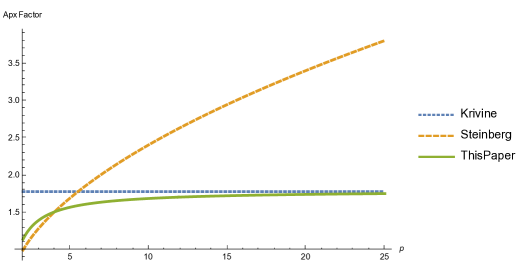
Figure 2: A comparison of the bounds for approximating $p{\rightarrow}p^{*}$ norm obtained from Krivine’s rounding for $K_{G}$, Steinberg’s analysis, and our bound. While our analysis yields an improved bound for $4\leq p\leq 66$, we believe that the rounding algorithm achieves an improved bound for all $p$.

Perhaps more interestingly, the above theorem is proved via a generalization of hyperplane rounding, which we believe may be of independent interest. Indeed, for a given collection of vectors $w^{1},\ldots,w^{m}$ considered as rows of a matrix $W$, Gaussian hyperplane rounding corresponds to taking the “rounded” solution $y$ to be the

$$y~{}:=~{}\operatorname*{\arg\!\max}_{\mathchoice{\lVert y^{\prime}\rVert_{\infty}}{\lVert y^{\prime}\rVert_{\infty}}{\lVert y^{\prime}\rVert_{\infty}}{\lVert y^{\prime}\rVert_{\infty}}\leq 1}\left\langle y^{\prime},W{\bf g}\right\rangle~{}=~{}\left(\operatorname{\operatorname{sgn}}\left(\left\langle w^{i},{\bf g}\right\rangle\right)\right)_{i\in[m]}\,.$$

We consider the natural generalization to (say) $\ell_{r}$ norms, given by

$$y~{}:=~{}\operatorname*{\arg\!\max}_{\mathchoice{\lVert y^{\prime}\rVert_{r}}{\lVert y^{\prime}\rVert_{r}}{\lVert y^{\prime}\rVert_{r}}{\lVert y^{\prime}\rVert_{r}}\leq 1}\left\langle y^{\prime},W{\bf g}\right\rangle~{}=~{}\left(\frac{\operatorname{\operatorname{sgn}}\left(\left\langle w^{i},{\bf g}\right\rangle\right)\cdot\left\lvert\langle w^{i},{\bf g}\rangle\right\rvert^{r^{*}-1}}{{\lVert W{\bf g}\rVert^{r^{*}-1}_{r^{*}}}}\right)_{i\in[m]}\,.$$

We refer to $y$ as the “Hölder dual” of $W{\bf g}$, since the above rounding can be obtained by viewing $W{\bf g}$ as lying in the dual ($\ell_{r^{*}}$) ball, and finding the $y$ for which Hölder’s inequality is tight. Indeed, in the above language, Nesterov’s rounding corresponds to considering the $\ell_{\infty}$ ball (hyperplane rounding). While Steinberg used a somewhat different relaxation, the rounding there can be obtained by viewing $W{\bf g}$ as lying in the primal $(\ell_{r})$ ball instead of the dual one. In case of hyperplane rounding, the analysis is motivated by the identity that for two unit vectors $u$ and $v$, we have

$$\mathchoice{\underset{{\bf g}}{\mathbb{E}}\left[\operatorname{\operatorname{sgn}}(\left\langle{\bf g},u\right\rangle)\cdot\operatorname{\operatorname{sgn}}(\left\langle{\bf g},v\right\rangle)\right]}{{\mathbb{E}}_{{\bf g}}[\operatorname{\operatorname{sgn}}(\left\langle{\bf g},u\right\rangle)\cdot\operatorname{\operatorname{sgn}}(\left\langle{\bf g},v\right\rangle)]}{{\mathbb{E}}_{{\bf g}}[\operatorname{\operatorname{sgn}}(\left\langle{\bf g},u\right\rangle)\cdot\operatorname{\operatorname{sgn}}(\left\langle{\bf g},v\right\rangle)]}{{\mathbb{E}}_{{\bf g}}[\operatorname{\operatorname{sgn}}(\left\langle{\bf g},u\right\rangle)\cdot\operatorname{\operatorname{sgn}}(\left\langle{\bf g},v\right\rangle)]}~{}=~{}\frac{2}{\pi}\cdot\sin^{-1}(\left\langle u,v\right\rangle)\,.$$

We prove the appropriate extension of this identity to $\ell_{r}$ balls (and analyze the functions arising there) which may also be of interest for other optimization problems over $\ell_{r}$ balls.

1.2 Proof overview

As discussed above, we consider Nesterov’s convex relaxation and generalize the hyperplane rounding scheme using “Hölder duals” of the Gaussian projections, instead of taking the sign. As in the Krivine rounding scheme, this rounding is applied to transformations of the SDP solutions. The nature of these transformations depends on how the rounding procedure changes the correlation between two vectors. Let $u,v\in{\mathbb{R}}^{N}$ be two unit vectors with $\left\langle u,v\right\rangle=\rho$. Then, for ${\bf g}\sim{\mathcal{N}(0,I_{N})}$, $\left\langle{\bf g},u\right\rangle$ and $\left\langle{\bf g},v\right\rangle$ are $\rho$-correlated Gaussian random variables. Hyperplane rounding then gives $\pm 1$ valued random variables whose correlation is given by

$$\mathchoice{\underset{{\bf g}_{1}\sim_{\rho}\,{\bf g}_{2}}{\mathbb{E}}\left[\operatorname{\operatorname{sgn}}({\bf g}_{1})\cdot\operatorname{\operatorname{sgn}}({\bf g}_{2})\right]}{{\mathbb{E}}_{{\bf g}_{1}\sim_{\rho}\,{\bf g}_{2}}[\operatorname{\operatorname{sgn}}({\bf g}_{1})\cdot\operatorname{\operatorname{sgn}}({\bf g}_{2})]}{{\mathbb{E}}_{{\bf g}_{1}\sim_{\rho}\,{\bf g}_{2}}[\operatorname{\operatorname{sgn}}({\bf g}_{1})\cdot\operatorname{\operatorname{sgn}}({\bf g}_{2})]}{{\mathbb{E}}_{{\bf g}_{1}\sim_{\rho}\,{\bf g}_{2}}[\operatorname{\operatorname{sgn}}({\bf g}_{1})\cdot\operatorname{\operatorname{sgn}}({\bf g}_{2})]}~{}=~{}\frac{2}{\pi}\cdot\sin^{-1}(\rho)\,.$$

The transformations $\varphi$ and $\psi$ (to be applied to the vectors $u$ and $v$) in Krivine’s scheme are then chosen depending on the Taylor series for the $\sin$ function, which is the inverse of function computed on the correlation. For the case of Hölder-dual rounding, we prove the following generalization of the above identity

$$\mathchoice{\underset{{\bf g}_{1}\sim_{\rho}\,{\bf g}_{2}}{\mathbb{E}}\left[\operatorname{\operatorname{sgn}}({\bf g}_{1})\left\lvert{\bf g}_{1}\right\rvert^{q-1}\cdot\operatorname{\operatorname{sgn}}({\bf g}_{2})\left\lvert{\bf g}_{2}\right\rvert^{p^{*}-1}\right]}{{\mathbb{E}}_{{\bf g}_{1}\sim_{\rho}\,{\bf g}_{2}}[\operatorname{\operatorname{sgn}}({\bf g}_{1})\left\lvert{\bf g}_{1}\right\rvert^{q-1}\cdot\operatorname{\operatorname{sgn}}({\bf g}_{2})\left\lvert{\bf g}_{2}\right\rvert^{p^{*}-1}]}{{\mathbb{E}}_{{\bf g}_{1}\sim_{\rho}\,{\bf g}_{2}}[\operatorname{\operatorname{sgn}}({\bf g}_{1})\left\lvert{\bf g}_{1}\right\rvert^{q-1}\cdot\operatorname{\operatorname{sgn}}({\bf g}_{2})\left\lvert{\bf g}_{2}\right\rvert^{p^{*}-1}]}{{\mathbb{E}}_{{\bf g}_{1}\sim_{\rho}\,{\bf g}_{2}}[\operatorname{\operatorname{sgn}}({\bf g}_{1})\left\lvert{\bf g}_{1}\right\rvert^{q-1}\cdot\operatorname{\operatorname{sgn}}({\bf g}_{2})\left\lvert{\bf g}_{2}\right\rvert^{p^{*}-1}]}~{}=~{}\gamma_{q}^{q}\cdot\gamma_{p^{*}}^{p^{*}}\cdot\rho\cdot{}_{2}F_{1}\!\left(1-\frac{q}{2},1-\frac{p^{*}}{2}\,;\,\frac{3}{2}\,;\,\rho^{2}\right)\,,$$

where ${}_{2}F_{1}$ denotes a hypergeometric function with the specified parameters. The proof of the above identity combines simple tools from Hermite analysis with known integral representations from the theory of special functions, and may be useful in other applications of the rounding procedure.

Note that in the Grothendieck case, we have $\gamma_{p^{*}}^{p^{*}}=\gamma_{q}^{q}=\sqrt{2/\pi}$, and the remaining part is simply the $\sin^{-1}$ function. In the Krivine rounding scheme, the transformations $\varphi$ and $\psi$ are chosen to satisfy $(2/\pi)\cdot\sin^{-1}\left(\left\langle\varphi(u),\psi(v)\right\rangle\right)=c\cdot\left\langle u,v\right\rangle$, where the constant $c$ then governs the approximation ratio. The transformations $\varphi(u)$ and $\psi(v)$ taken to be of the form $\varphi(u)=\oplus_{i=1}^{\infty}a_{i}\cdot u^{\otimes i}$ such that

$$\left\langle\varphi(u),\psi(v)\right\rangle~{}=~{}c^{\prime}\cdot\sin\left(\left\langle u,v\right\rangle\right)\qquad\text{and}\qquad\mathchoice{\lVert\varphi(u)\rVert_{2}}{\lVert\varphi(u)\rVert_{2}}{\lVert\varphi(u)\rVert_{2}}{\lVert\varphi(u)\rVert_{2}}=\mathchoice{\lVert\psi(v)\rVert}{\lVert\psi(v)\rVert}{\lVert\psi(v)\rVert}{\lVert\psi(v)\rVert}=1\,.$$

If $f$ represents (a normalized version of) the function of $\rho$ occurring in the identity above (which is $\sin^{-1}$ for hyperplane rounding), then the approximation ratio is governed by the function $h$ obtained by replacing every Taylor coefficient of $f^{-1}$ by its absolute value. While $f^{-1}$ is simply the $\sin$ function (and thus $h$ is the $\sinh$ function) in the Grothendieck problem, no closed-form expressions are available for general $p$ and $q$.

The task of understanding the approximation ratio thus reduces to the analytic task of understanding the family of the functions $h$ obtained for different values of $p$ and $q$. Concretely, the approximation ratio is given by the value $1/(h^{-1}(1)\cdot\gamma_{q}\,\gamma_{p^{*}})$. At a high level, we prove bounds on $h^{-1}(1)$ by establishing properties of the Taylor coefficients of the family of functions $f^{-1}$, i.e., the family given by

$$\left\{f^{-1}~{}~{}|~{}~{}f(\rho)=\rho\cdot{}_{2}F_{1}\!\left(a_{1},b_{1}\,;\,3/2\,;\,\rho^{2}\right)~{},~{}a_{1},b_{1}\in[0,1/2]\right\}\,.$$

While in the cases considered earlier, the functions $h$ are easy to determine in terms of $f^{-1}$ via succinct formulae [Kri77, Haa81, AN04] or can be truncated after the cubic term [NR14], neither of these are true for the family of functions we consider. Hypergeometric functions are a rich and expressive class of functions, capturing many of the special functions appearing in Mathematical Physics and various ensembles of orthogonal polynomials. Due to this expressive power, the set of inverses is not well understood. In particular, while the coefficients of $f$ are monotone in $p$ and $q$, this is not true for $f^{-1}$. Moreover, the rates of decay of the coefficients may range from inverse polynomial to super-exponential. We analyze the coefficients of $f^{-1}$ using complex-analytic methods inspired by (but quite different from) the work of Haagerup [Haa81] on bounding the complex Grothendieck constant. The key technical challenge in our work is in arguing systematically about a family of inverse hypergeometric functions which we address by developing methods to estimate the values of a family of contour integrals.

While our method only gives a bound of the form $h^{-1}(1)\geq\sinh^{-1}(1)/(1+\varepsilon_{0})$, we believe this is an artifact of the analysis and the true bound should indeed be $h^{-1}(1)\geq\sinh^{-1}(1)$.

1.3 Relation to Factorization Theory

Let $X,Y$ be Banach spaces, and let $A:X\rightarrow Y$ be a continuous linear operator. As before, the norm $\mathchoice{\lVert A\rVert_{X\rightarrow Y}}{\lVert A\rVert_{X\rightarrow Y}}{\lVert A\rVert_{X\rightarrow Y}}{\lVert A\rVert_{X\rightarrow Y}}$ is defined as

$$\mathchoice{\lVert A\rVert_{X\rightarrow Y}}{\lVert A\rVert_{X\rightarrow Y}}{\lVert A\rVert_{X\rightarrow Y}}{\lVert A\rVert_{X\rightarrow Y}}~{}:=~{}\sup_{x\in X\setminus\{0\}}\frac{\mathchoice{\lVert Ax\rVert_{Y}}{\lVert Ax\rVert_{Y}}{\lVert Ax\rVert_{Y}}{\lVert Ax\rVert_{Y}}}{\mathchoice{\lVert x\rVert_{X}}{\lVert x\rVert_{X}}{\lVert x\rVert_{X}}{\lVert x\rVert_{X}}}\,.$$

The operator $A$ is said to be factorize through Hilbert space if the factorization constant of $A$ defined as

$$\Phi(A)~{}:=~{}\inf_{H}\inf_{BC=A}\frac{\mathchoice{\lVert C\rVert_{X\rightarrow H}}{\lVert C\rVert_{X\rightarrow H}}{\lVert C\rVert_{X\rightarrow H}}{\lVert C\rVert_{X\rightarrow H}}\cdot\mathchoice{\lVert B\rVert_{H\rightarrow Y}}{\lVert B\rVert_{H\rightarrow Y}}{\lVert B\rVert_{H\rightarrow Y}}{\lVert B\rVert_{H\rightarrow Y}}}{\mathchoice{\lVert A\rVert_{X\rightarrow Y}}{\lVert A\rVert_{X\rightarrow Y}}{\lVert A\rVert_{X\rightarrow Y}}{\lVert A\rVert_{X\rightarrow Y}}}$$

is bounded, where the infimum is taken over all Hilbert spaces $H$ and all operators $B:H\rightarrow Y$ and $C:X\rightarrow H$. The factorization gap for spaces $X$ and $Y$ is then defined as $\Phi(X,Y):=\sup_{A}\Phi(A)$ where the supremum runs over all continuous operators $A:X\rightarrow Y$.

The theory of factorization of linear operators is a cornerstone of modern functional analysis and has also found many applications outside the field (see [Pis86, AK06] for more information). An application to theoretical computer science was found by Tropp [Tro09] who used the Grothendieck factorization [Gro56] to give an algorithmic version of a celebrated column subset selection result of Bourgain and Tzafriri [BT87].

As an almost immediate consequence of convex programming duality, our new algorithmic results also imply some improved factorization results for $\ell_{p}^{n},\ell_{q}^{m}$. We first state some classical factorization results, for which we will use $T_{2}(X)$ and $C_{2}(X)$ to respectively denote the Type-2 and Cotype-2 constants of $X$. We refer the interested reader to Appendix A for a more detailed description of factorization theory as well as the relevant functional analysis preliminaries.

The Kwapień-Maurey [Kwa72a, Mau74] theorem states that for any pair of Banach spaces $X$ and $Y$

$$\Phi(X,Y)~{}\leq~{}T_{2}(X)\cdot C_{2}(Y)\,.$$

However, Grothendieck’s result [Gro56] shows that a much better bound is possible in a case where $T_{2}(X)$ is unbounded. In particular,

$$\Phi(\ell_{\infty}^{n},\ell_{1}^{m})~{}\leq~{}K_{G}\,,$$

for all $m,n\in{\mathbb{N}}$. Pisier [Pis80] showed that if $X$ or $Y$ satisfies the approximation property (which is always satisfied by finite-dimensional spaces), then

$$\Phi(X,Y)~{}\leq~{}\left(2\cdot C_{2}(X^{*})\cdot C_{2}(Y)\right)^{3/2}\,.$$

We show that the approximation ratio of Nesterov’s relaxation is in fact an upper bound on the factorization gap for the spaces $\ell_{p}^{n}$ and $\ell_{q}^{m}$. Combined with our upper bound on the integrality gap, we show an improved bound on the factorization constant, i.e., for any $p\geq 2\geq q$ and $m,n\in{\mathbb{N}}$, we have that for $X=\ell_{p}^{n}$, $Y=\ell_{q}^{m}$

$$\Phi(X,Y)~{}\leq~{}\frac{1+\varepsilon_{0}}{\sinh^{-1}(1)}\cdot\left(C_{2}(X^{*})\cdot C_{2}(Y)\right)\,,$$

where $\varepsilon_{0}\leq 0.00863$ as before. This improves on Pisier’s bound for all $p\geq 2\geq q$, and for certain ranges of $(p,q)$ it also improves upon $K_{G}$ and the bound of Kwapień-Maurey.

1.4 Approximability and Factorizability

Let $(X_{n})$ and $(Y_{m})$ be sequences of Banach spaces such that $X_{n}$ is over the vector space ${\mathbb{R}}^{n}$ and $Y_{m}$ is over the vector space ${\mathbb{R}}^{m}$. We shall say a pair of sequences $((X_{n}),(Y_{m}))$ factorize if $\Phi(X_{n},Y_{m})$ is bounded by a constant independent of $m$ and $n$. Similarly, we shall say a pair of families $((X_{n}),(Y_{m}))$ are computationally approximable if there exists a polynomial $R(m,n)$, such that for every $m,n\in{\mathbb{N}}$, there is an algorithm with runtime $R(m,n)$ approximating $\mathchoice{\lVert A\rVert_{X_{n}\rightarrow Y_{m}}}{\lVert A\rVert_{X_{n}\rightarrow Y_{m}}}{\lVert A\rVert_{X_{n}\rightarrow Y_{m}}}{\lVert A\rVert_{X_{n}\rightarrow Y_{m}}}$ within a constant independent of $m$ and $n$ (given an oracle for computing the norms of vectors and a separation oracle for the unit balls of the norms). We consider the natural question of characterizing the families of norms that are approximable and their connection to factorizability and Cotype.

The pairs $(p,q)$ (assuming $p^{*},q\neq\infty$) for which $(\ell_{p}^{n},\ell_{q}^{m})$ is known (resp. not known) to factorize, are precisely those pairs $(p,q)$ which are known to be computationally approximable (resp. inapproximable assuming hardness conjectures like $\textrm{P}\neq\textsf{NP}$ and ETH). Moreover the Hilbertian case which trivially satisfies factorizability, is also known to be computationally approximable (with approximation factor 1).

It is tempting to ask whether the set of computationally approximable pairs is closely related to the set of factorizable pairs or the pairs for which $X^{*}_{n},Y_{m}$ have bounded (independent of $m,n$) Cotype-2 constant. Further yet, is there a connection between the approximation factor and the factorization constant, or approximation factor and Cotype-2 constants (of $X_{n}^{*}$ and $Y_{m}$)? Our work gives some modest additional evidence towards such conjectures. Such a result would give credibility to the appealing intuitive idea of the approximation factor being dependent on the “distance” to a Hilbert space.

1.5 Notation

For a non-negative real number $r$, we define the $r$-th Gaussian norm of a standard gaussian $g$ as $\gamma_{r}:=(\mathchoice{\underset{g\sim{\mathcal{N}(0,1)}}{\mathbb{E}}\left[\left\lvert g\right\rvert^{r}\right]}{{\mathbb{E}}_{g\sim{\mathcal{N}(0,1)}}[\left\lvert g\right\rvert^{r}]}{{\mathbb{E}}_{g\sim{\mathcal{N}(0,1)}}[\left\lvert g\right\rvert^{r}]}{{\mathbb{E}}_{g\sim{\mathcal{N}(0,1)}}[\left\lvert g\right\rvert^{r}]})^{\nicefrac{{1}}{{r}}}\,.$

Given a vector $x$, we define the $r$-norm as ${\lVert x\rVert^{r}_{r}}=\sum_{i}{\left\lvert x_{i}\right\rvert^{r}}$ for all $r\geq 1$. For any $r\geq 0$, we denote the dual norm by $r^{*}$, which satisfies the equality: $\frac{1}{r}+\frac{1}{r^{*}}=1$.

For $p\geq 2\geq q\geq 1$, we will use the following notation: $a:=p^{*}-1$ and $b:=q-1$. We note that $a,b\in[0,1]$.

For a $m\times n$ matrix $M$ (or vector, when $n=1$). For an unitary function $f$, we define $f[M]$ to be the matrix $M$ with entries defined as $(f[M])_{i,j}=f(M_{i,j})$ for $i\in[m],j\in[n]$. For vectors $u,v\in{\mathbb{R}}^{\ell}$, we denote by $u\circ v\in{\mathbb{R}}^{\ell}$ the entry-wise/Hadamard product of $u$ and $v$. We denote the concatenation of two vectors $u$ and $v$ by $u\oplus v$. For a vector $u$, we use $D_{u}$ to denote the diagonal matrix with the entries of $u$ forming the diagonal, and for a matrix $M$ we use $\operatorname{\operatorname{diag}}(M)$ to denote the vector of diagonal entries.

For a function $f(\tau)=\sum_{k\geq 0}f_{k}\cdot\tau^{k}$ defined as a power series, we denote the function $\mathrm{abs}\left(f\right)(\tau):=\sum_{k\geq 0}\left\lvert f_{k}\right\rvert\cdot\tau^{k}$.

2 Analyzing the Approximation Ratio via Rounding

We will show that $\mathsf{CP}(A)$ is a good approximation to $\mathchoice{\lVert A\rVert_{p\rightarrow q}}{\lVert A\rVert_{p\rightarrow q}}{\lVert A\rVert_{p\rightarrow q}}{\lVert A\rVert_{p\rightarrow q}}$ by using an appropriate generalization of Krivine’s rounding procedure. Before stating the generalized procedure, we shall give a more detailed summary of Krivine’s procedure.

2.1 Krivine’s Rounding Procedure

Krivine’s procedure centers around the classical random hyperplane rounding. In this context, we define the random hyperplane rounding procedure on an input pair of matrices $U\in{\mathbb{R}}^{m\times\ell},~{}V\in{\mathbb{R}}^{n\times\ell}$ as outputting the vectors $\operatorname{\operatorname{sgn}}[U{\bf g}]$ and $\operatorname{\operatorname{sgn}}[V{\bf g}]$ where ${\bf g}\in{\mathbb{R}}^{\ell}$ is a vector with i.i.d. standard Gaussian coordinates ($f[v]$ denotes entry-wise application of a scalar function $f$ to a vector $v$. We use the same convention for matrices.). The so-called Grothendieck identity states that for vectors $u,v\in{\mathbb{R}}^{\ell}$,

$$\mathchoice{{\mathbb{E}}\left[\operatorname{\operatorname{sgn}}\!{\langle{\bf g}\,,u\rangle}\cdot\operatorname{\operatorname{sgn}}\!{\langle{\bf g}\,,v\rangle}\right]}{{\mathbb{E}}[\operatorname{\operatorname{sgn}}\!{\langle{\bf g}\,,u\rangle}\cdot\operatorname{\operatorname{sgn}}\!{\langle{\bf g}\,,v\rangle}]}{{\mathbb{E}}[\operatorname{\operatorname{sgn}}\!{\langle{\bf g}\,,u\rangle}\cdot\operatorname{\operatorname{sgn}}\!{\langle{\bf g}\,,v\rangle}]}{{\mathbb{E}}[\operatorname{\operatorname{sgn}}\!{\langle{\bf g}\,,u\rangle}\cdot\operatorname{\operatorname{sgn}}\!{\langle{\bf g}\,,v\rangle}]}=\frac{\sin^{-1}\!{\langle\widehat{u}\,,\widehat{v}\rangle}}{\pi/2}$$

where $\widehat{u}$ denotes $u/\mathchoice{\lVert u\rVert_{2}}{\lVert u\rVert_{2}}{\lVert u\rVert_{2}}{\lVert u\rVert_{2}}$. This implies the following equality which we will call the hyperplane rounding identity:

$$\mathchoice{{\mathbb{E}}\left[\operatorname{\operatorname{sgn}}[U{\bf g}](\operatorname{\operatorname{sgn}}[V{\bf g}])^{T}\right]}{{\mathbb{E}}[\operatorname{\operatorname{sgn}}[U{\bf g}](\operatorname{\operatorname{sgn}}[V{\bf g}])^{T}]}{{\mathbb{E}}[\operatorname{\operatorname{sgn}}[U{\bf g}](\operatorname{\operatorname{sgn}}[V{\bf g}])^{T}]}{{\mathbb{E}}[\operatorname{\operatorname{sgn}}[U{\bf g}](\operatorname{\operatorname{sgn}}[V{\bf g}])^{T}]}=\frac{\sin^{-1}[\widehat{U}\widehat{V}^{T}]}{\pi/2}\,.$$ (1)

where for a matrix $U$, we use $\widehat{U}$ to denote the matrix obtained by replacing the rows of $U$ by the corresponding unit (in $\ell_{2}$ norm) vectors. Krivine’s main observation is that for any matrices $U,V$, there exist matrices $\varphi(\widehat{U}),\psi(\widehat{V})$ with unit vectors as rows, such that

$$\varphi(\widehat{U})\,\psi(\widehat{V})^{T}=\sin[(\pi/2)\cdot c\cdot\widehat{U}\widehat{V}^{T}]$$

where $c=\sinh^{-1}(1)\cdot 2/\pi$. Taking $\widehat{U},\widehat{V}$ to be the optimal solution to $\mathsf{CP}(A)$, it follows that

$$\mathchoice{\lVert A\rVert_{\infty\rightarrow 1}}{\lVert A\rVert_{\infty\rightarrow 1}}{\lVert A\rVert_{\infty\rightarrow 1}}{\lVert A\rVert_{\infty\rightarrow 1}}\geq\left\langle A\,,\mathchoice{{\mathbb{E}}\left[\operatorname{\operatorname{sgn}}[\varphi(\widehat{U})\,{\bf g}]~{}(\operatorname{\operatorname{sgn}}[\psi(\widehat{V})\,{\bf g}])^{T}\right]}{{\mathbb{E}}[\operatorname{\operatorname{sgn}}[\varphi(\widehat{U})\,{\bf g}]~{}(\operatorname{\operatorname{sgn}}[\psi(\widehat{V})\,{\bf g}])^{T}]}{{\mathbb{E}}[\operatorname{\operatorname{sgn}}[\varphi(\widehat{U})\,{\bf g}]~{}(\operatorname{\operatorname{sgn}}[\psi(\widehat{V})\,{\bf g}])^{T}]}{{\mathbb{E}}[\operatorname{\operatorname{sgn}}[\varphi(\widehat{U})\,{\bf g}]~{}(\operatorname{\operatorname{sgn}}[\psi(\widehat{V})\,{\bf g}])^{T}]}\right\rangle=\langle A\,,c\cdot\widehat{U}\widehat{V}^{T}\rangle=c\cdot\mathsf{CP}(A)\,.$$

The proof of Krivine’s observation follows from simulating the Taylor series of a scalar function using inner products. We will now describe this more concretely.

Observation 2.1 (Krivine).

Let $f:[-1,1]\rightarrow{\mathbb{R}}$ be a scalar function satisfying $f(\rho)=\sum_{k\geq 1}f_{k}\,\rho^{k}$ for an absolutely convergent series $(f_{k})$. Let $\mathrm{abs}\left(f\right)(\rho):=\sum_{k\geq 1}|f_{k}|\,\rho^{k}$ and further for vectors $u,v\in{\mathbb{R}}^{\ell}$ of $\ell_{2}$-length at most $1$, let

$$S_{L}(f,u):=(\operatorname{\operatorname{sgn}}(f_{1})\sqrt{f_{1}}\cdot u)\oplus(\operatorname{\operatorname{sgn}}(f_{2})\sqrt{f_{2}}\cdot u^{\otimes 2})\oplus(\operatorname{\operatorname{sgn}}(f_{3})\sqrt{f_{3}}\cdot u^{\otimes 3})\oplus\cdots$$

$$S_{R}(f,v):=(\sqrt{f_{1}}\cdot v)\oplus(\sqrt{f_{2}}\cdot v^{\otimes 2})\oplus(\sqrt{f_{3}}\cdot v^{\otimes 3})\oplus\cdots$$

Then for any $U\in{\mathbb{R}}^{m\times\ell},~{}V\in{\mathbb{R}}^{n\times\ell}$,  $S_{L}(f,\sqrt{c_{f}}\cdot\widehat{U})$ and $S_{R}(f,\sqrt{c_{f}}\cdot\widehat{V})$ have $\ell_{2}$-unit vectors as rows, and

$$S_{L}(f,\sqrt{c_{f}}\cdot\widehat{U})~{}S_{R}(f,\sqrt{c_{f}}\cdot\widehat{V})^{T}=f\,[c_{f}\cdot\widehat{U}\widehat{V}^{T}]$$

where $S_{L}(f,W)$ for a matrix $W$, is applied to row-wise and $c_{f}:=(\mathrm{abs}\left(f\right)^{-1})(1)$.

Proof.

Using the facts $\langle y^{1}\otimes y^{2}\,,y^{3}\otimes y^{4}\rangle=\langle y^{1}\,,y^{3}\rangle\cdot\langle y^{2}\,,y^{4}\rangle$ and
$\langle y^{1}\oplus y^{2}\,,y^{3}\oplus y^{4}\rangle=\langle y^{1}\,,y^{3}\rangle+\langle y^{2}\,,y^{4}\rangle$, we have

• $\langle S_{L}(f,u)\,,S_{R}(f,v)\rangle=f(\langle u\,,v\rangle)$

• $\mathchoice{\lVert S_{L}(f,u)\rVert_{2}}{\lVert S_{L}(f,u)\rVert_{2}}{\lVert S_{L}(f,u)\rVert_{2}}{\lVert S_{L}(f,u)\rVert_{2}}=\sqrt{\mathrm{abs}\left(f\right)({\lVert u\rVert^{2}_{2}})}$

• $\mathchoice{\lVert S_{R}(f,v)\rVert_{2}}{\lVert S_{R}(f,v)\rVert_{2}}{\lVert S_{R}(f,v)\rVert_{2}}{\lVert S_{R}(f,v)\rVert_{2}}=\sqrt{\mathrm{abs}\left(f\right)({\lVert v\rVert^{2}_{2}})}$

The claim follows.      

Before stating our full rounding procedure, we first discuss a natural generalization of random hyperplane rounding, and much like in Krivine’s case this will guide the final procedure.

2.2 Generalizing Random Hyperplane Rounding – Hölder Dual Rounding

Fix any convex bodies $B_{1}\subset{\mathbb{R}}^{m}$ and $B_{2}\subset{\mathbb{R}}^{k}$. Suppose that we would like a strategy that for given vectors $y\in{\mathbb{R}}^{m},~{}x\in{\mathbb{R}}^{n}$, outputs $\overline{y}\in B_{1},~{}\overline{x}\in B_{2}$ so that $y^{T}A\,x=\langle A\,,y\,x^{T}\rangle$ is close to $\langle A\,,\overline{y}\,\overline{x}^{T}\rangle$ for all $A$. A natural strategy is to take

$$(\overline{y},\overline{x}):=\operatorname*{\arg\!\max}_{(\widetilde{y},\widetilde{x})\in B_{1}\times B_{2}}\left\langle\widetilde{y}\,\widetilde{x}^{T}\,,y\,x^{T}\right\rangle=\left(\operatorname*{\arg\!\max}_{\widetilde{y}\in B_{1}}\left\langle\widetilde{y}\,,y\right\rangle~{},~{}\operatorname*{\arg\!\max}_{\widetilde{x}\in B_{2}}\left\langle\widetilde{x}\,,x\right\rangle\right)$$

In the special case where $B$ is the unit $\ell_{p}$ ball, there is a closed form for an optimal solution to $\max_{\widetilde{x}\in B}\langle\widetilde{x}\,,x\rangle$, given by $\Psi_{\!p^{*}}(x)/{\lVert x\rVert^{p^{*}-1}_{p^{*}}}$, where $\Psi_{\!p^{*}}(x):=\operatorname{\operatorname{sgn}}[x]\circ|[x]|^{p^{*}-1}$. Note that for $p=\infty$, this strategy recovers the random hyperplane rounding procedure. We shall call this procedure, Gaussian Hölder Dual Rounding or Hölder Dual Rounding for short.

Just like earlier, we will first understand the effect of Hölder Dual Rounding on a solution pair $U,V$. For $\rho\in[-1,1]$, let ${\bf g}_{1}\!\sim_{\rho}{\bf g}_{2}$ denote $\rho$-correlated standard Gaussians, i.e., ${\bf g}_{1}=\rho\,{\bf g}_{2}+\sqrt{1-\rho^{2}}\,{\bf g}_{3}$  where $({\bf g}_{2},{\bf g}_{3})\sim{\mathcal{N}(0,\mathrm{I}_{2})}$, and let

$$\widetilde{f}_{a,\,b}(\rho):=\mathchoice{\underset{{\bf g}_{1}\sim_{\rho}{\bf g}_{2}}{\mathbb{E}}\left[\operatorname{\operatorname{sgn}}({\bf g}_{1})|{\bf g}_{1}|^{b}\operatorname{\operatorname{sgn}}({\bf g}_{2})|{\bf g}_{1}|^{a}\right]}{{\mathbb{E}}_{{\bf g}_{1}\sim_{\rho}{\bf g}_{2}}[\operatorname{\operatorname{sgn}}({\bf g}_{1})|{\bf g}_{1}|^{b}\operatorname{\operatorname{sgn}}({\bf g}_{2})|{\bf g}_{1}|^{a}]}{{\mathbb{E}}_{{\bf g}_{1}\sim_{\rho}{\bf g}_{2}}[\operatorname{\operatorname{sgn}}({\bf g}_{1})|{\bf g}_{1}|^{b}\operatorname{\operatorname{sgn}}({\bf g}_{2})|{\bf g}_{1}|^{a}]}{{\mathbb{E}}_{{\bf g}_{1}\sim_{\rho}{\bf g}_{2}}[\operatorname{\operatorname{sgn}}({\bf g}_{1})|{\bf g}_{1}|^{b}\operatorname{\operatorname{sgn}}({\bf g}_{2})|{\bf g}_{1}|^{a}]}$$

We will work towards a better understanding of $\widetilde{f}_{a,\,b}(\cdot)$ in later sections. For now note that we have for vectors $u,v\in{\mathbb{R}}^{\ell}$,

$$\mathchoice{{\mathbb{E}}\left[\operatorname{\operatorname{sgn}}\!{\langle{\bf g}\,,u\rangle}\,|\langle{\bf g}\,,u\rangle|^{b}\cdot\operatorname{\operatorname{sgn}}\!{\langle{\bf g}\,,v\rangle}\,|\langle{\bf g}\,,v\rangle|^{a}\right]}{{\mathbb{E}}[\operatorname{\operatorname{sgn}}\!{\langle{\bf g}\,,u\rangle}\,|\langle{\bf g}\,,u\rangle|^{b}\cdot\operatorname{\operatorname{sgn}}\!{\langle{\bf g}\,,v\rangle}\,|\langle{\bf g}\,,v\rangle|^{a}]}{{\mathbb{E}}[\operatorname{\operatorname{sgn}}\!{\langle{\bf g}\,,u\rangle}\,|\langle{\bf g}\,,u\rangle|^{b}\cdot\operatorname{\operatorname{sgn}}\!{\langle{\bf g}\,,v\rangle}\,|\langle{\bf g}\,,v\rangle|^{a}]}{{\mathbb{E}}[\operatorname{\operatorname{sgn}}\!{\langle{\bf g}\,,u\rangle}\,|\langle{\bf g}\,,u\rangle|^{b}\cdot\operatorname{\operatorname{sgn}}\!{\langle{\bf g}\,,v\rangle}\,|\langle{\bf g}\,,v\rangle|^{a}]}={\lVert u\rVert^{b}_{2}}\cdot{\lVert v\rVert^{a}_{2}}\cdot\widetilde{f}_{a,\,b}(\langle\widehat{u}\,,\widehat{v}\,\rangle)\,.$$

Thus given matrices $U,V$, we obtain the following generalization of the hyperplane rounding identity for Hölder Dual Rounding :

$$\mathchoice{{\mathbb{E}}\left[\Psi_{\!q}([U{\bf g}])\,\Psi_{\!p^{*}}([V{\bf g}])^{T}\right]}{{\mathbb{E}}[\Psi_{\!q}([U{\bf g}])\,\Psi_{\!p^{*}}([V{\bf g}])^{T}]}{{\mathbb{E}}[\Psi_{\!q}([U{\bf g}])\,\Psi_{\!p^{*}}([V{\bf g}])^{T}]}{{\mathbb{E}}[\Psi_{\!q}([U{\bf g}])\,\Psi_{\!p^{*}}([V{\bf g}])^{T}]}=D_{({\lVert u^{i}\rVert^{b}_{2}})_{i\in[m]}}\cdot\widetilde{f}_{a,\,b}([\widehat{U}\widehat{V}^{T}])\cdot D_{({\lVert v^{j}\rVert^{a}_{2}})_{j\in[n]}}\,.$$ (2)

2.3 Generalized Krivine Transformation and the Full Rounding Procedure

We are finally ready to state the generalized version of Krivine’s algorithm. At a high level the algorithm simply applies Hölder Dual Rounding to a transformed version of the optimal convex program solution pair $U,V$. Analogous to Krivine’s algorithm, the transformation is a type of “inverse” of Eq. 2.

1. Let $(U,V)$ be the optimal solution to $\mathsf{CP}(A)$, and let $(u^{i})_{i\in[m]}$ and $(v^{j})_{j\in[n]}$ respectively denote the rows of $U$ and $V$.

2. Let $c_{a,b}:=\left(\mathrm{abs}\left(\widetilde{f}^{-1}_{a,\,b}\right)\right)^{-1}\!\!(1)$ and let

   $$\varphi(U) :=D_{({\lVert u^{i}\rVert^{1/b}_{2}})_{i\in[m]}}\,\,S_{L}(\widetilde{f}^{-1}_{a,\,b},\sqrt{c_{a,b}}\cdot\widehat{U})\,,$$

   $$\psi(V) :=D_{({\lVert v^{j}\rVert^{1/a}_{2}})_{j\in[n]}}\,\,S_{R}(\widetilde{f}^{-1}_{a,\,b},\sqrt{c_{a,b}}\cdot\widehat{V})\,.$$

1. Let ${\bf g}\sim{\mathcal{N}(0,\mathrm{I})}$ be an infinite dimensional i.i.d. Gaussian vector.

2. Return $y:=\Psi_{\!q}(\varphi(U)\,{\bf g})/{\lVert\varphi(U)\,{\bf g}\rVert^{b}_{q}}$ and $x:=\Psi_{\!p^{*}}(\psi(V)\,{\bf g})/{\lVert\psi(V)\,{\bf g}\rVert^{a}_{p^{*}}}$.

Remark 2.2.

Note that $\mathchoice{\lVert\Psi_{\!r}(\overline{x})\rVert_{r^{*}}}{\lVert\Psi_{\!r}(\overline{x})\rVert_{r^{*}}}{\lVert\Psi_{\!r}(\overline{x})\rVert_{r^{*}}}{\lVert\Psi_{\!r}(\overline{x})\rVert_{r^{*}}}={\lVert\overline{x}\rVert^{r-1}_{r}}$ and so the returned solution pair always lie on the unit $\ell_{q^{*}}$ and $\ell_{p}$ spheres respectively.

Remark 2.3.

Like in [AN04] the procedure above can be made algorithmic by observing that there always exist $\varphi^{\prime}(U)\in{\mathbb{R}}^{m\times(m+n)}$ and $\psi^{\prime}(V)\in{\mathbb{R}}^{m\times(m+n)}$, whose rows have the exact same lengths and pairwise inner products as those of $\varphi(U)$ and $\psi(V)$ above. Moreover they can be computed without explicitly computing $\varphi(U)$ and $\psi(V)$ by obtaining the Gram decomposition of

$$M~{}:=~{}\left[\begin{array}[]{cc}\mathrm{abs}\left(\widetilde{f}^{-1}_{a,\,b}\right)[c_{a,b}\cdot\widehat{V}\widehat{V}^{T}]&\widetilde{f}^{-1}_{a,\,b}([c_{a,b}\cdot\widehat{U}\widehat{V}^{T}])\\ \widetilde{f}^{-1}_{a,\,b}([c_{a,b}\cdot\widehat{V}\widehat{U}^{T}])&\mathrm{abs}\left(\widetilde{f}^{-1}_{a,\,b}\right)[c_{a,b}\cdot\widehat{V}\widehat{V}^{T}]\end{array}\right]\,,$$

and normalizing the rows of the decomposition according to the definition of $\varphi(\cdot)$ and $\psi(\cdot)$ above. The entries of $M$ can be computed in polynomial time with exponentially (in $m$ and $n$) good accuracy by implementing the Taylor series of $\widetilde{f}^{-1}_{a,\,b}$ upto $\mathrm{poly}(m,n)$ terms (Taylor series inversion can be done upto $k$ terms in time $\mathrm{poly}(k)$).

Remark 2.4.

Note that the $2$-norm of the $i$-th row (resp. $j$-th row) of $\varphi(U)$ (resp. $\psi(V)$) is ${\lVert u^{i}\rVert^{1/b}_{2}}$ (resp. ${\lVert v^{j}\rVert^{1/a}_{2}}$).

We commence the analysis by defining some convenient normalized functions and we will also show that $c_{a,b}$ above is well-defined.

2.4 Auxiliary Functions

Let  $f_{p,\,q}(\rho):=\widetilde{f}_{p,\,q}(\rho)/(\gamma_{p^{*}}^{p^{*}}\,\gamma_{q}^{q})$,   $\widetilde{h}_{a,\,b}:=\mathrm{abs}\left(\widetilde{f}^{-1}_{a,\,b}\right)$,  and  $h_{a,\,b}:=\mathrm{abs}\left(f^{-1}_{a,\,b}\right)$. Also note that $h^{-1}_{a,\,b}(\rho)=\widetilde{h}^{-1}_{a,\,b}(\rho)/(\gamma_{p^{*}}^{p^{*}}\,\gamma_{q}^{q})$.

Well Definedness.

By Lemma 4.7, $f^{-1}_{a,\,b}(\rho)$ and $h_{a,\,b}(\rho)$ are well defined for $\rho\in[-1,1]$. By (M1) in Corollary 3.19,   $\widetilde{f}^{-1}_{1}=1$ and hence $h_{a,\,b}(1)\geq 1$ and $h_{a,\,b}(-1)\leq-1$. Combining this with the fact that $h_{a,\,b}(\rho)$ is continuous and strictly increasing on $[-1,1]$, implies that $h^{-1}_{a,\,b}(x)$ is well defined on $[-1,1]$.

We can now proceed with the analysis.

2.5 $1/(h^{-1}_{p,\,q}(1)\cdot\gamma_{p^{*}}\,\gamma_{q})$ Bound on Approximation Factor

For any vector random variable $\mathbf{X}$ in a universe $\Omega$, and scalar valued functions $f_{1}:\Omega\rightarrow{\mathbb{R}}$ and $f_{2}:\Omega\rightarrow(0,\infty)$. Let $\lambda=\mathchoice{{\mathbb{E}}\left[f_{1}(\mathbf{X})\right]}{{\mathbb{E}}[f_{1}(\mathbf{X})]}{{\mathbb{E}}[f_{1}(\mathbf{X})]}{{\mathbb{E}}[f_{1}(\mathbf{X})]}/\mathchoice{{\mathbb{E}}\left[f_{2}(\mathbf{X})\right]}{{\mathbb{E}}[f_{2}(\mathbf{X})]}{{\mathbb{E}}[f_{2}(\mathbf{X})]}{{\mathbb{E}}[f_{2}(\mathbf{X})]}$. Now we have

$$\max_{x\in\Omega}f_{1}(x)-\lambda\cdot f_{2}(x)\geq\mathchoice{{\mathbb{E}}\left[f_{1}(\mathbf{X})-\lambda\cdot f_{2}(\mathbf{X})\right]}{{\mathbb{E}}[f_{1}(\mathbf{X})-\lambda\cdot f_{2}(\mathbf{X})]}{{\mathbb{E}}[f_{1}(\mathbf{X})-\lambda\cdot f_{2}(\mathbf{X})]}{{\mathbb{E}}[f_{1}(\mathbf{X})-\lambda\cdot f_{2}(\mathbf{X})]}=0$$

$$\Rightarrow\quad \max_{x\in\Omega}f_{1}(x)/f_{2}(x)\geq\lambda=\mathchoice{{\mathbb{E}}\left[f_{1}(\mathbf{X})\right]}{{\mathbb{E}}[f_{1}(\mathbf{X})]}{{\mathbb{E}}[f_{1}(\mathbf{X})]}{{\mathbb{E}}[f_{1}(\mathbf{X})]}/\mathchoice{{\mathbb{E}}\left[f_{2}(\mathbf{X})\right]}{{\mathbb{E}}[f_{2}(\mathbf{X})]}{{\mathbb{E}}[f_{2}(\mathbf{X})]}{{\mathbb{E}}[f_{2}(\mathbf{X})]}\,.$$

Thus we have

$$\mathchoice{\lVert A\rVert_{p\rightarrow q}}{\lVert A\rVert_{p\rightarrow q}}{\lVert A\rVert_{p\rightarrow q}}{\lVert A\rVert_{p\rightarrow q}}~{}\geq~{}\frac{\mathchoice{{\mathbb{E}}\left[\langle A\,,\Psi_{\!q}(\varphi(U)\,{\bf g})~{}\Psi_{\!p^{*}}(\psi(V)\,{\bf g})^{T}\rangle\right]}{{\mathbb{E}}[\langle A\,,\Psi_{\!q}(\varphi(U)\,{\bf g})~{}\Psi_{\!p^{*}}(\psi(V)\,{\bf g})^{T}\rangle]}{{\mathbb{E}}[\langle A\,,\Psi_{\!q}(\varphi(U)\,{\bf g})~{}\Psi_{\!p^{*}}(\psi(V)\,{\bf g})^{T}\rangle]}{{\mathbb{E}}[\langle A\,,\Psi_{\!q}(\varphi(U)\,{\bf g})~{}\Psi_{\!p^{*}}(\psi(V)\,{\bf g})^{T}\rangle]}}{\mathchoice{{\mathbb{E}}\left[\mathchoice{\lVert\Psi_{\!q}(\varphi(U)\,{\bf g})\rVert_{q^{*}}}{\lVert\Psi_{\!q}(\varphi(U)\,{\bf g})\rVert_{q^{*}}}{\lVert\Psi_{\!q}(\varphi(U)\,{\bf g})\rVert_{q^{*}}}{\lVert\Psi_{\!q}(\varphi(U)\,{\bf g})\rVert_{q^{*}}}\cdot\mathchoice{\lVert\Psi_{\!p^{*}}(\psi(V)\,{\bf g})\rVert_{p}}{\lVert\Psi_{\!p^{*}}(\psi(V)\,{\bf g})\rVert_{p}}{\lVert\Psi_{\!p^{*}}(\psi(V)\,{\bf g})\rVert_{p}}{\lVert\Psi_{\!p^{*}}(\psi(V)\,{\bf g})\rVert_{p}}\right]}{{\mathbb{E}}[\mathchoice{\lVert\Psi_{\!q}(\varphi(U)\,{\bf g})\rVert_{q^{*}}}{\lVert\Psi_{\!q}(\varphi(U)\,{\bf g})\rVert_{q^{*}}}{\lVert\Psi_{\!q}(\varphi(U)\,{\bf g})\rVert_{q^{*}}}{\lVert\Psi_{\!q}(\varphi(U)\,{\bf g})\rVert_{q^{*}}}\cdot\mathchoice{\lVert\Psi_{\!p^{*}}(\psi(V)\,{\bf g})\rVert_{p}}{\lVert\Psi_{\!p^{*}}(\psi(V)\,{\bf g})\rVert_{p}}{\lVert\Psi_{\!p^{*}}(\psi(V)\,{\bf g})\rVert_{p}}{\lVert\Psi_{\!p^{*}}(\psi(V)\,{\bf g})\rVert_{p}}]}{{\mathbb{E}}[\mathchoice{\lVert\Psi_{\!q}(\varphi(U)\,{\bf g})\rVert_{q^{*}}}{\lVert\Psi_{\!q}(\varphi(U)\,{\bf g})\rVert_{q^{*}}}{\lVert\Psi_{\!q}(\varphi(U)\,{\bf g})\rVert_{q^{*}}}{\lVert\Psi_{\!q}(\varphi(U)\,{\bf g})\rVert_{q^{*}}}\cdot\mathchoice{\lVert\Psi_{\!p^{*}}(\psi(V)\,{\bf g})\rVert_{p}}{\lVert\Psi_{\!p^{*}}(\psi(V)\,{\bf g})\rVert_{p}}{\lVert\Psi_{\!p^{*}}(\psi(V)\,{\bf g})\rVert_{p}}{\lVert\Psi_{\!p^{*}}(\psi(V)\,{\bf g})\rVert_{p}}]}{{\mathbb{E}}[\mathchoice{\lVert\Psi_{\!q}(\varphi(U)\,{\bf g})\rVert_{q^{*}}}{\lVert\Psi_{\!q}(\varphi(U)\,{\bf g})\rVert_{q^{*}}}{\lVert\Psi_{\!q}(\varphi(U)\,{\bf g})\rVert_{q^{*}}}{\lVert\Psi_{\!q}(\varphi(U)\,{\bf g})\rVert_{q^{*}}}\cdot\mathchoice{\lVert\Psi_{\!p^{*}}(\psi(V)\,{\bf g})\rVert_{p}}{\lVert\Psi_{\!p^{*}}(\psi(V)\,{\bf g})\rVert_{p}}{\lVert\Psi_{\!p^{*}}(\psi(V)\,{\bf g})\rVert_{p}}{\lVert\Psi_{\!p^{*}}(\psi(V)\,{\bf g})\rVert_{p}}]}}~{}=~{}\frac{\langle A\,,\mathchoice{{\mathbb{E}}\left[\Psi_{\!q}(\varphi(U)\,{\bf g})~{}\Psi_{\!p^{*}}(\psi(V)\,{\bf g})^{T}\right]}{{\mathbb{E}}[\Psi_{\!q}(\varphi(U)\,{\bf g})~{}\Psi_{\!p^{*}}(\psi(V)\,{\bf g})^{T}]}{{\mathbb{E}}[\Psi_{\!q}(\varphi(U)\,{\bf g})~{}\Psi_{\!p^{*}}(\psi(V)\,{\bf g})^{T}]}{{\mathbb{E}}[\Psi_{\!q}(\varphi(U)\,{\bf g})~{}\Psi_{\!p^{*}}(\psi(V)\,{\bf g})^{T}]}\rangle}{\mathchoice{{\mathbb{E}}\left[\mathchoice{\lVert\Psi_{\!q}(\varphi(U)\,{\bf g})\rVert_{q^{*}}}{\lVert\Psi_{\!q}(\varphi(U)\,{\bf g})\rVert_{q^{*}}}{\lVert\Psi_{\!q}(\varphi(U)\,{\bf g})\rVert_{q^{*}}}{\lVert\Psi_{\!q}(\varphi(U)\,{\bf g})\rVert_{q^{*}}}\cdot\mathchoice{\lVert\Psi_{\!p^{*}}(\psi(V)\,{\bf g})\rVert_{p}}{\lVert\Psi_{\!p^{*}}(\psi(V)\,{\bf g})\rVert_{p}}{\lVert\Psi_{\!p^{*}}(\psi(V)\,{\bf g})\rVert_{p}}{\lVert\Psi_{\!p^{*}}(\psi(V)\,{\bf g})\rVert_{p}}\right]}{{\mathbb{E}}[\mathchoice{\lVert\Psi_{\!q}(\varphi(U)\,{\bf g})\rVert_{q^{*}}}{\lVert\Psi_{\!q}(\varphi(U)\,{\bf g})\rVert_{q^{*}}}{\lVert\Psi_{\!q}(\varphi(U)\,{\bf g})\rVert_{q^{*}}}{\lVert\Psi_{\!q}(\varphi(U)\,{\bf g})\rVert_{q^{*}}}\cdot\mathchoice{\lVert\Psi_{\!p^{*}}(\psi(V)\,{\bf g})\rVert_{p}}{\lVert\Psi_{\!p^{*}}(\psi(V)\,{\bf g})\rVert_{p}}{\lVert\Psi_{\!p^{*}}(\psi(V)\,{\bf g})\rVert_{p}}{\lVert\Psi_{\!p^{*}}(\psi(V)\,{\bf g})\rVert_{p}}]}{{\mathbb{E}}[\mathchoice{\lVert\Psi_{\!q}(\varphi(U)\,{\bf g})\rVert_{q^{*}}}{\lVert\Psi_{\!q}(\varphi(U)\,{\bf g})\rVert_{q^{*}}}{\lVert\Psi_{\!q}(\varphi(U)\,{\bf g})\rVert_{q^{*}}}{\lVert\Psi_{\!q}(\varphi(U)\,{\bf g})\rVert_{q^{*}}}\cdot\mathchoice{\lVert\Psi_{\!p^{*}}(\psi(V)\,{\bf g})\rVert_{p}}{\lVert\Psi_{\!p^{*}}(\psi(V)\,{\bf g})\rVert_{p}}{\lVert\Psi_{\!p^{*}}(\psi(V)\,{\bf g})\rVert_{p}}{\lVert\Psi_{\!p^{*}}(\psi(V)\,{\bf g})\rVert_{p}}]}{{\mathbb{E}}[\mathchoice{\lVert\Psi_{\!q}(\varphi(U)\,{\bf g})\rVert_{q^{*}}}{\lVert\Psi_{\!q}(\varphi(U)\,{\bf g})\rVert_{q^{*}}}{\lVert\Psi_{\!q}(\varphi(U)\,{\bf g})\rVert_{q^{*}}}{\lVert\Psi_{\!q}(\varphi(U)\,{\bf g})\rVert_{q^{*}}}\cdot\mathchoice{\lVert\Psi_{\!p^{*}}(\psi(V)\,{\bf g})\rVert_{p}}{\lVert\Psi_{\!p^{*}}(\psi(V)\,{\bf g})\rVert_{p}}{\lVert\Psi_{\!p^{*}}(\psi(V)\,{\bf g})\rVert_{p}}{\lVert\Psi_{\!p^{*}}(\psi(V)\,{\bf g})\rVert_{p}}]}}\,,$$

which allows us to consider the numerator and denominator separately. We begin by proving the equality that the above algorithm was designed to satisfy:

Lemma 2.5.

$\mathchoice{{\mathbb{E}}\left[\Psi_{\!q}(\varphi(U)\,{\bf g})~{}\Psi_{\!p^{*}}(\psi(V)\,{\bf g})^{T}\right]}{{\mathbb{E}}[\Psi_{\!q}(\varphi(U)\,{\bf g})~{}\Psi_{\!p^{*}}(\psi(V)\,{\bf g})^{T}]}{{\mathbb{E}}[\Psi_{\!q}(\varphi(U)\,{\bf g})~{}\Psi_{\!p^{*}}(\psi(V)\,{\bf g})^{T}]}{{\mathbb{E}}[\Psi_{\!q}(\varphi(U)\,{\bf g})~{}\Psi_{\!p^{*}}(\psi(V)\,{\bf g})^{T}]}~{}=~{}c_{a,b}\cdot(\widetilde{U}\widetilde{V}^{T})$

Proof.

$$\quad~{}~{}\mathchoice{{\mathbb{E}}\left[\Psi_{\!q}(\varphi(U)\,{\bf g})~{}\Psi_{\!p^{*}}(\psi(V)\,{\bf g})^{T}\right]}{{\mathbb{E}}[\Psi_{\!q}(\varphi(U)\,{\bf g})~{}\Psi_{\!p^{*}}(\psi(V)\,{\bf g})^{T}]}{{\mathbb{E}}[\Psi_{\!q}(\varphi(U)\,{\bf g})~{}\Psi_{\!p^{*}}(\psi(V)\,{\bf g})^{T}]}{{\mathbb{E}}[\Psi_{\!q}(\varphi(U)\,{\bf g})~{}\Psi_{\!p^{*}}(\psi(V)\,{\bf g})^{T}]}$$

$$=D_{(\mathchoice{\lVert u^{i}\rVert_{2}}{\lVert u^{i}\rVert_{2}}{\lVert u^{i}\rVert_{2}}{\lVert u^{i}\rVert_{2}})_{i\in[m]}}\cdot\widetilde{f}_{a,\,b}([S_{L}(\widetilde{f}^{-1}_{a,\,b},\sqrt{c_{a,b}}\cdot\widehat{U})\cdot S_{R}(\widetilde{f}^{-1}_{a,\,b},\sqrt{c_{a,b}}\cdot\widehat{V})^{T}])\cdot D_{(\mathchoice{\lVert v^{j}\rVert_{2}}{\lVert v^{j}\rVert_{2}}{\lVert v^{j}\rVert_{2}}{\lVert v^{j}\rVert_{2}})_{j\in[n]}}$$

$$~{}~{}(\text{by \lx@cref{creftype~refnum}{cvgp:identity} and \lx@cref{creftype~refnum}{algo:rmk}})$$

$$=D_{(\mathchoice{\lVert u^{i}\rVert_{2}}{\lVert u^{i}\rVert_{2}}{\lVert u^{i}\rVert_{2}}{\lVert u^{i}\rVert_{2}})_{i\in[m]}}\cdot\widetilde{f}_{a,\,b}([\widetilde{f}^{-1}_{a,\,b}([c_{a,b}\cdot\widehat{U}\widehat{V}^{T}])])\cdot D_{(\mathchoice{\lVert v^{j}\rVert_{2}}{\lVert v^{j}\rVert_{2}}{\lVert v^{j}\rVert_{2}}{\lVert v^{j}\rVert_{2}})_{j\in[n]}}$$

$$~{}~{}(\text{by \lx@cref{creftype~refnum}{simulating:taylor}})$$

$$=D_{(\mathchoice{\lVert u^{i}\rVert_{2}}{\lVert u^{i}\rVert_{2}}{\lVert u^{i}\rVert_{2}}{\lVert u^{i}\rVert_{2}})_{i\in[m]}}\cdot c_{a,b}\cdot\widehat{U}\widehat{V}^{T}\cdot D_{(\mathchoice{\lVert v^{j}\rVert_{2}}{\lVert v^{j}\rVert_{2}}{\lVert v^{j}\rVert_{2}}{\lVert v^{j}\rVert_{2}})_{j\in[n]}}$$

$$=c_{a,b}\cdot UV^{T} \blacksquare$$

It remains to upper bound the denominator which we do using a straightforward convexity argument.

Lemma 2.6.

$\mathchoice{{\mathbb{E}}\left[{\lVert\varphi(U)\,{\bf g}\rVert^{b}_{q}}\cdot{\lVert\psi(V)\,{\bf g}\rVert^{a}_{p^{*}}}\right]}{{\mathbb{E}}[{\lVert\varphi(U)\,{\bf g}\rVert^{b}_{q}}\cdot{\lVert\psi(V)\,{\bf g}\rVert^{a}_{p^{*}}}]}{{\mathbb{E}}[{\lVert\varphi(U)\,{\bf g}\rVert^{b}_{q}}\cdot{\lVert\psi(V)\,{\bf g}\rVert^{a}_{p^{*}}}]}{{\mathbb{E}}[{\lVert\varphi(U)\,{\bf g}\rVert^{b}_{q}}\cdot{\lVert\psi(V)\,{\bf g}\rVert^{a}_{p^{*}}}]}\leq\gamma_{p^{*}}^{a}\,\gamma_{q}^{b}\,.$

Proof.

$$\quad~{}\mathchoice{{\mathbb{E}}\left[{\lVert\varphi(U)\,{\bf g}\rVert^{b}_{q}}\cdot{\lVert\psi(V)\,{\bf g}\rVert^{a}_{p^{*}}}\right]}{{\mathbb{E}}[{\lVert\varphi(U)\,{\bf g}\rVert^{b}_{q}}\cdot{\lVert\psi(V)\,{\bf g}\rVert^{a}_{p^{*}}}]}{{\mathbb{E}}[{\lVert\varphi(U)\,{\bf g}\rVert^{b}_{q}}\cdot{\lVert\psi(V)\,{\bf g}\rVert^{a}_{p^{*}}}]}{{\mathbb{E}}[{\lVert\varphi(U)\,{\bf g}\rVert^{b}_{q}}\cdot{\lVert\psi(V)\,{\bf g}\rVert^{a}_{p^{*}}}]}$$

$$\leq~{}\mathchoice{{\mathbb{E}}\left[{\lVert\varphi(U)\,{\bf g}\rVert^{q^{*}b}_{q}}\right]}{{\mathbb{E}}[{\lVert\varphi(U)\,{\bf g}\rVert^{q^{*}b}_{q}}]}{{\mathbb{E}}[{\lVert\varphi(U)\,{\bf g}\rVert^{q^{*}b}_{q}}]}{{\mathbb{E}}[{\lVert\varphi(U)\,{\bf g}\rVert^{q^{*}b}_{q}}]}\!^{1/q^{*}}\cdot\mathchoice{{\mathbb{E}}\left[{\lVert\psi(V)\,{\bf g}\rVert^{pa}_{p^{*}}}\right]}{{\mathbb{E}}[{\lVert\psi(V)\,{\bf g}\rVert^{pa}_{p^{*}}}]}{{\mathbb{E}}[{\lVert\psi(V)\,{\bf g}\rVert^{pa}_{p^{*}}}]}{{\mathbb{E}}[{\lVert\psi(V)\,{\bf g}\rVert^{pa}_{p^{*}}}]}\!^{1/p} \left(\frac{1}{p}+\frac{1}{q^{*}}\leq 1\right)$$

$$=~{}\mathchoice{{\mathbb{E}}\left[{\lVert\varphi(U)\,{\bf g}\rVert^{q}_{q}}\right]}{{\mathbb{E}}[{\lVert\varphi(U)\,{\bf g}\rVert^{q}_{q}}]}{{\mathbb{E}}[{\lVert\varphi(U)\,{\bf g}\rVert^{q}_{q}}]}{{\mathbb{E}}[{\lVert\varphi(U)\,{\bf g}\rVert^{q}_{q}}]}\!^{1/q^{*}}\cdot\mathchoice{{\mathbb{E}}\left[{\lVert\psi(V)\,{\bf g}\rVert^{p^{*}}_{p^{*}}}\right]}{{\mathbb{E}}[{\lVert\psi(V)\,{\bf g}\rVert^{p^{*}}_{p^{*}}}]}{{\mathbb{E}}[{\lVert\psi(V)\,{\bf g}\rVert^{p^{*}}_{p^{*}}}]}{{\mathbb{E}}[{\lVert\psi(V)\,{\bf g}\rVert^{p^{*}}_{p^{*}}}]}\!^{1/p}$$

$$=~{}\left[\sum_{i\in[m]}\mathchoice{{\mathbb{E}}\left[|{\mathcal{N}(0,{\lVert u^{i}\rVert^{1/b}_{2}})}|^{q}\right]}{{\mathbb{E}}[|{\mathcal{N}(0,{\lVert u^{i}\rVert^{1/b}_{2}})}|^{q}]}{{\mathbb{E}}[|{\mathcal{N}(0,{\lVert u^{i}\rVert^{1/b}_{2}})}|^{q}]}{{\mathbb{E}}[|{\mathcal{N}(0,{\lVert u^{i}\rVert^{1/b}_{2}})}|^{q}]}\right]^{1/q^{*}}\cdot\left[\sum_{j\in[n]}\mathchoice{{\mathbb{E}}\left[|{\mathcal{N}(0,{\lVert v^{j}\rVert^{1/a}_{2}})}|^{p^{*}}\right]}{{\mathbb{E}}[|{\mathcal{N}(0,{\lVert v^{j}\rVert^{1/a}_{2}})}|^{p^{*}}]}{{\mathbb{E}}[|{\mathcal{N}(0,{\lVert v^{j}\rVert^{1/a}_{2}})}|^{p^{*}}]}{{\mathbb{E}}[|{\mathcal{N}(0,{\lVert v^{j}\rVert^{1/a}_{2}})}|^{p^{*}}]}\right]^{1/p} (\text{By \lx@cref{creftype~refnum}{algo:rmk}})$$

$$=~{}\left[\sum_{i\in[m]}{\lVert u^{i}\rVert^{q/b}_{2}}\right]^{1/q^{*}}\cdot\left[\sum_{j\in[n]}{\lVert v^{j}\rVert^{p^{*}/a}_{2}}\right]^{1/p}\cdot\gamma_{q}^{q/q^{*}}\,\gamma_{p^{*}}^{p^{*}/p}$$

$$=~{}\left[\sum_{i\in[m]}{\lVert u^{i}\rVert^{q^{*}}_{2}}\right]^{1/q^{*}}\cdot\left[\sum_{j\in[n]}{\lVert v^{j}\rVert^{p}_{2}}\right]^{1/p}\cdot\gamma_{q}^{b}\,\gamma_{p^{*}}^{a}$$

$$=~{}\gamma_{q}^{b}\,\gamma_{p^{*}}^{a} (\text{feasibility of }U,V)\qquad\hbox{\vrule width=6.0pt,height=6.0pt,depth=0.0pt}$$

We are now ready to prove our approximation guarantee.

Lemma 2.7.

Consider any $1\leq q\leq 2\leq p\leq\infty$. Then,

$$\frac{\mathsf{CP}(A)}{\mathchoice{\lVert A\rVert_{p\rightarrow q}}{\lVert A\rVert_{p\rightarrow q}}{\lVert A\rVert_{p\rightarrow q}}{\lVert A\rVert_{p\rightarrow q}}}~{}\leq~{}1/(\gamma_{p^{*}}\,\gamma_{q}\cdot h^{-1}_{a,\,b}(1))$$

Proof.

$$\mathchoice{\lVert A\rVert_{p\rightarrow q}}{\lVert A\rVert_{p\rightarrow q}}{\lVert A\rVert_{p\rightarrow q}}{\lVert A\rVert_{p\rightarrow q}}~{} \geq~{}\frac{\langle A\,,\mathchoice{{\mathbb{E}}\left[\Psi_{\!q}(\varphi(U)\,{\bf g})~{}\Psi_{\!p^{*}}(\psi(V)\,{\bf g})^{T}\right]}{{\mathbb{E}}[\Psi_{\!q}(\varphi(U)\,{\bf g})~{}\Psi_{\!p^{*}}(\psi(V)\,{\bf g})^{T}]}{{\mathbb{E}}[\Psi_{\!q}(\varphi(U)\,{\bf g})~{}\Psi_{\!p^{*}}(\psi(V)\,{\bf g})^{T}]}{{\mathbb{E}}[\Psi_{\!q}(\varphi(U)\,{\bf g})~{}\Psi_{\!p^{*}}(\psi(V)\,{\bf g})^{T}]}\rangle}{\mathchoice{{\mathbb{E}}\left[\mathchoice{\lVert\Psi_{\!q}(\varphi(U)\,{\bf g})\rVert_{q^{*}}}{\lVert\Psi_{\!q}(\varphi(U)\,{\bf g})\rVert_{q^{*}}}{\lVert\Psi_{\!q}(\varphi(U)\,{\bf g})\rVert_{q^{*}}}{\lVert\Psi_{\!q}(\varphi(U)\,{\bf g})\rVert_{q^{*}}}\cdot\mathchoice{\lVert\Psi_{\!p^{*}}(\psi(V)\,{\bf g})\rVert_{p}}{\lVert\Psi_{\!p^{*}}(\psi(V)\,{\bf g})\rVert_{p}}{\lVert\Psi_{\!p^{*}}(\psi(V)\,{\bf g})\rVert_{p}}{\lVert\Psi_{\!p^{*}}(\psi(V)\,{\bf g})\rVert_{p}}\right]}{{\mathbb{E}}[\mathchoice{\lVert\Psi_{\!q}(\varphi(U)\,{\bf g})\rVert_{q^{*}}}{\lVert\Psi_{\!q}(\varphi(U)\,{\bf g})\rVert_{q^{*}}}{\lVert\Psi_{\!q}(\varphi(U)\,{\bf g})\rVert_{q^{*}}}{\lVert\Psi_{\!q}(\varphi(U)\,{\bf g})\rVert_{q^{*}}}\cdot\mathchoice{\lVert\Psi_{\!p^{*}}(\psi(V)\,{\bf g})\rVert_{p}}{\lVert\Psi_{\!p^{*}}(\psi(V)\,{\bf g})\rVert_{p}}{\lVert\Psi_{\!p^{*}}(\psi(V)\,{\bf g})\rVert_{p}}{\lVert\Psi_{\!p^{*}}(\psi(V)\,{\bf g})\rVert_{p}}]}{{\mathbb{E}}[\mathchoice{\lVert\Psi_{\!q}(\varphi(U)\,{\bf g})\rVert_{q^{*}}}{\lVert\Psi_{\!q}(\varphi(U)\,{\bf g})\rVert_{q^{*}}}{\lVert\Psi_{\!q}(\varphi(U)\,{\bf g})\rVert_{q^{*}}}{\lVert\Psi_{\!q}(\varphi(U)\,{\bf g})\rVert_{q^{*}}}\cdot\mathchoice{\lVert\Psi_{\!p^{*}}(\psi(V)\,{\bf g})\rVert_{p}}{\lVert\Psi_{\!p^{*}}(\psi(V)\,{\bf g})\rVert_{p}}{\lVert\Psi_{\!p^{*}}(\psi(V)\,{\bf g})\rVert_{p}}{\lVert\Psi_{\!p^{*}}(\psi(V)\,{\bf g})\rVert_{p}}]}{{\mathbb{E}}[\mathchoice{\lVert\Psi_{\!q}(\varphi(U)\,{\bf g})\rVert_{q^{*}}}{\lVert\Psi_{\!q}(\varphi(U)\,{\bf g})\rVert_{q^{*}}}{\lVert\Psi_{\!q}(\varphi(U)\,{\bf g})\rVert_{q^{*}}}{\lVert\Psi_{\!q}(\varphi(U)\,{\bf g})\rVert_{q^{*}}}\cdot\mathchoice{\lVert\Psi_{\!p^{*}}(\psi(V)\,{\bf g})\rVert_{p}}{\lVert\Psi_{\!p^{*}}(\psi(V)\,{\bf g})\rVert_{p}}{\lVert\Psi_{\!p^{*}}(\psi(V)\,{\bf g})\rVert_{p}}{\lVert\Psi_{\!p^{*}}(\psi(V)\,{\bf g})\rVert_{p}}]}}$$

$$=~{}\frac{\langle A\,,\mathchoice{{\mathbb{E}}\left[\Psi_{\!q}(\varphi(U)\,{\bf g})~{}\Psi_{\!p^{*}}(\psi(V)\,{\bf g})^{T}\right]}{{\mathbb{E}}[\Psi_{\!q}(\varphi(U)\,{\bf g})~{}\Psi_{\!p^{*}}(\psi(V)\,{\bf g})^{T}]}{{\mathbb{E}}[\Psi_{\!q}(\varphi(U)\,{\bf g})~{}\Psi_{\!p^{*}}(\psi(V)\,{\bf g})^{T}]}{{\mathbb{E}}[\Psi_{\!q}(\varphi(U)\,{\bf g})~{}\Psi_{\!p^{*}}(\psi(V)\,{\bf g})^{T}]}\rangle}{\mathchoice{{\mathbb{E}}\left[{\lVert\varphi(U)\,{\bf g}\rVert^{b}_{q}}\cdot{\lVert\psi(V)\,{\bf g}\rVert^{a}_{p^{*}}}\right]}{{\mathbb{E}}[{\lVert\varphi(U)\,{\bf g}\rVert^{b}_{q}}\cdot{\lVert\psi(V)\,{\bf g}\rVert^{a}_{p^{*}}}]}{{\mathbb{E}}[{\lVert\varphi(U)\,{\bf g}\rVert^{b}_{q}}\cdot{\lVert\psi(V)\,{\bf g}\rVert^{a}_{p^{*}}}]}{{\mathbb{E}}[{\lVert\varphi(U)\,{\bf g}\rVert^{b}_{q}}\cdot{\lVert\psi(V)\,{\bf g}\rVert^{a}_{p^{*}}}]}} (\text{by \lx@cref{creftype~refnum}{round:feasibility}})$$

$$=~{}\frac{c_{a,b}\cdot\langle A\,,UV^{T}\rangle}{\mathchoice{{\mathbb{E}}\left[{\lVert\varphi(U)\,{\bf g}\rVert^{b}_{q}}\cdot{\lVert\psi(V)\,{\bf g}\rVert^{a}_{p^{*}}}\right]}{{\mathbb{E}}[{\lVert\varphi(U)\,{\bf g}\rVert^{b}_{q}}\cdot{\lVert\psi(V)\,{\bf g}\rVert^{a}_{p^{*}}}]}{{\mathbb{E}}[{\lVert\varphi(U)\,{\bf g}\rVert^{b}_{q}}\cdot{\lVert\psi(V)\,{\bf g}\rVert^{a}_{p^{*}}}]}{{\mathbb{E}}[{\lVert\varphi(U)\,{\bf g}\rVert^{b}_{q}}\cdot{\lVert\psi(V)\,{\bf g}\rVert^{a}_{p^{*}}}]}} (\text{by \lx@cref{creftype~refnum}{numerator}})$$

$$=~{}\frac{c_{a,b}\cdot\mathsf{CP}(A)}{\mathchoice{{\mathbb{E}}\left[{\lVert\varphi(U)\,{\bf g}\rVert^{b}_{q}}\cdot{\lVert\psi(V)\,{\bf g}\rVert^{a}_{p^{*}}}\right]}{{\mathbb{E}}[{\lVert\varphi(U)\,{\bf g}\rVert^{b}_{q}}\cdot{\lVert\psi(V)\,{\bf g}\rVert^{a}_{p^{*}}}]}{{\mathbb{E}}[{\lVert\varphi(U)\,{\bf g}\rVert^{b}_{q}}\cdot{\lVert\psi(V)\,{\bf g}\rVert^{a}_{p^{*}}}]}{{\mathbb{E}}[{\lVert\varphi(U)\,{\bf g}\rVert^{b}_{q}}\cdot{\lVert\psi(V)\,{\bf g}\rVert^{a}_{p^{*}}}]}} (\text{by optimality of }U,V)$$

$$\geq~{}\frac{c_{a,b}\cdot\mathsf{CP}(A)}{\gamma_{p^{*}}^{a}\,\gamma_{q}^{b}} (\text{by \lx@cref{creftype~refnum}{denominator}})$$

$$=~{}\frac{\widetilde{h}^{-1}_{a,\,b}(1)\cdot\mathsf{CP}(A)}{\gamma_{p^{*}}^{a}\,\gamma_{q}^{b}}$$

$$=~{}h^{-1}_{a,\,b}(1)\cdot\gamma_{p^{*}}\,\gamma_{q}\cdot\mathsf{CP}(A) \blacksquare$$

We next begin the primary technical undertaking of this paper, namely proving upper bounds on $h^{-1}_{p,\,q}(1)$.

3 Hypergeometric Representation of $f_{a,\,b}(x)$

In this section, we show that $f_{a,\,b}(\rho)$ can be represented using the Gaussian hypergeometric function ${}_{2}F_{1}$. The result of this section can be thought of as a generalization of the so-called Grothendieck identity for hyperplane rounding which simply states that

$$f_{0,\,0}(\rho)~{}=~{}\frac{\pi}{2}\cdot\mathchoice{\underset{{\bf g}_{1}\sim_{\rho}\,{\bf g}_{2}}{\mathbb{E}}\left[\operatorname{\operatorname{sgn}}({\bf g}_{1})\operatorname{\operatorname{sgn}}({\bf g}_{2})\right]}{{\mathbb{E}}_{{\bf g}_{1}\sim_{\rho}\,{\bf g}_{2}}[\operatorname{\operatorname{sgn}}({\bf g}_{1})\operatorname{\operatorname{sgn}}({\bf g}_{2})]}{{\mathbb{E}}_{{\bf g}_{1}\sim_{\rho}\,{\bf g}_{2}}[\operatorname{\operatorname{sgn}}({\bf g}_{1})\operatorname{\operatorname{sgn}}({\bf g}_{2})]}{{\mathbb{E}}_{{\bf g}_{1}\sim_{\rho}\,{\bf g}_{2}}[\operatorname{\operatorname{sgn}}({\bf g}_{1})\operatorname{\operatorname{sgn}}({\bf g}_{2})]}~{}=~{}\sin^{-1}(\rho)$$

We believe the result of this section and its proof technique to be of independent interest in analyzing generalizations of hyperplane rounding to convex bodies other than the hypercube.

Recall that $\widetilde{f}_{a,\,b}(\rho)$ is defined as follows:

$$\mathchoice{\underset{{\bf g}_{1}\sim_{\rho}\,{\bf g}_{2}}{\mathbb{E}}\left[\operatorname{\operatorname{sgn}}({\bf g}_{1})|{\bf g}_{1}|^{a}\operatorname{\operatorname{sgn}}({\bf g}_{2})|{\bf g}_{1}|^{b}\right]}{{\mathbb{E}}_{{\bf g}_{1}\sim_{\rho}\,{\bf g}_{2}}[\operatorname{\operatorname{sgn}}({\bf g}_{1})|{\bf g}_{1}|^{a}\operatorname{\operatorname{sgn}}({\bf g}_{2})|{\bf g}_{1}|^{b}]}{{\mathbb{E}}_{{\bf g}_{1}\sim_{\rho}\,{\bf g}_{2}}[\operatorname{\operatorname{sgn}}({\bf g}_{1})|{\bf g}_{1}|^{a}\operatorname{\operatorname{sgn}}({\bf g}_{2})|{\bf g}_{1}|^{b}]}{{\mathbb{E}}_{{\bf g}_{1}\sim_{\rho}\,{\bf g}_{2}}[\operatorname{\operatorname{sgn}}({\bf g}_{1})|{\bf g}_{1}|^{a}\operatorname{\operatorname{sgn}}({\bf g}_{2})|{\bf g}_{1}|^{b}]}$$

where $a=p^{*}-1$ and $b=q-1$. Our starting point is the simple observation that the above expectation can be viewed as the noise correlation (under the Gaussian measure) of the functions $\widetilde{f}^{\,(a)}(\tau):=\operatorname{\operatorname{sgn}}{\tau}\cdot|\tau|^{a}$ and $\widetilde{f}^{\,(b)}(\tau):=\operatorname{\operatorname{sgn}}{\tau}\cdot|\tau|^{b}$. Elementary Hermite analysis then implies that it suffices to understand the Hermite coefficients of $\widetilde{f}^{\,(a)}$ and $\widetilde{f}^{\,(b)}$ individually, in order to understand the Taylor coefficients of $f_{a,\,b}$. To understand the Hermite coefficients of $\widetilde{f}^{\,(a)}$ and $\widetilde{f}^{\,(b)}$ individually, we use a generating function approach. More specifically, we derive an integral representation for the generating function of the (appropriately normalized) Hermite coefficients which fortunately turns out to be closely related to a well studied special function called the parabolic cylinder function.

Before proceeding, we require some preliminaries.

3.1 Hermite Analysis Preliminaries

Let $\gamma$ denote the standard Gaussian probability distribution. For this section (and only for this section), the (Gaussian) inner product for functions $f,h\in({\mathbb{R}},\gamma)\rightarrow{\mathbb{R}}$ is defined as

$$\langle f\,,h\rangle:=\int_{{\mathbb{R}}}f(\tau)\cdot h(\tau)\,\,d\gamma(\tau)=\mathchoice{\underset{\tau\sim{\mathcal{N}(0,1)}}{\mathbb{E}}\left[f(\tau)\cdot h(\tau)\right]}{{\mathbb{E}}_{\tau\sim{\mathcal{N}(0,1)}}[f(\tau)\cdot h(\tau)]}{{\mathbb{E}}_{\tau\sim{\mathcal{N}(0,1)}}[f(\tau)\cdot h(\tau)]}{{\mathbb{E}}_{\tau\sim{\mathcal{N}(0,1)}}[f(\tau)\cdot h(\tau)]}\,.$$

Under this inner product there is a complete set of orthonormal polynomials $(H_{k})_{k\in{\mathbb{N}}}$ defined below.

Definition 3.1.

For a natural number $k$, then the $k$-th Hermite polynomial $H_{k}:{\mathbb{R}}\rightarrow{\mathbb{R}}$

$$H_{k}(\tau)=\frac{1}{\sqrt{k!}}\cdot(-1)^{\,k}\cdot\mathrm{e}^{\tau^{2}/2}\cdot\frac{d^{k}}{d\tau^{k}}\,\mathrm{e}^{-\tau^{2}/2}\,.$$

Any function $f$ satisfying $\int_{{\mathbb{R}}}|f(\tau)|^{2}\,d\gamma(\tau)<\infty$ has a Hermite expansion given by $f=\sum_{k\geq 0}\widehat{f}_{k}\cdot H_{k}$ where $\widehat{f}_{k}=\langle f\,,H_{k}\rangle\,.$

We have

Fact 3.2.

$H_{k}(\tau)$ is an even (resp. odd) function when $k$ is even (resp. odd).

We also have the Plancherel Identity (as Hermite polynomials form an orthonormal basis):

Fact 3.3.

For two real valued functions $f$ and $h$ with Hermite coefficients $\widehat{f}_{k}$ and $\widehat{h}_{k}$, respectively, we have:

$$\langle f\,,h\rangle=\sum_{k\geq 0}\widehat{f}_{k}\cdot\widehat{h}_{k}\,.$$

The generating function of appropriately normalized Hermite polynomials satisfies the following identity:

$$e^{\,\tau\lambda-\lambda^{2}/2}=\sum_{k\geq 0}H_{k}(\tau)\cdot\frac{\lambda^{k}}{\sqrt{k!}}\,.$$ (3)

Similar to the noise operator in Fourier analysis, we define the corresponding noise operator $T_{\rho}\,{}$ for Hermite analysis:

Definition 3.4.

For $\rho\in[-1,1]$ and a real valued function $f$, we define the function $T_{\rho}\,{f}$ as:

$$(T_{\rho}\,{f})(\tau)=\int_{{\mathbb{R}}}f\left(\rho\cdot\tau+\sqrt{1-\rho^{2}}\cdot\theta\right)\,d\gamma(\theta)=\mathchoice{\underset{\tau^{\prime}\sim_{\rho}\,\tau}{\mathbb{E}}\left[f(\tau^{\prime})\right]}{{\mathbb{E}}_{\tau^{\prime}\sim_{\rho}\,\tau}[f(\tau^{\prime})]}{{\mathbb{E}}_{\tau^{\prime}\sim_{\rho}\,\tau}[f(\tau^{\prime})]}{{\mathbb{E}}_{\tau^{\prime}\sim_{\rho}\,\tau}[f(\tau^{\prime})]}\,.$$

Again similar to the case of Fourier analysis, the Hermite coefficients admit the following identity:

Fact 3.5.

$\widehat{(T_{\rho}\,{f})}_{k}=\rho^{k}\cdot\widehat{f}_{k}\,.$

We recall that the $\widetilde{f}_{a,\,b}(\rho)=\mathchoice{\underset{{\bf g}_{1}\sim\rho\,{\bf g}_{2}}{\mathbb{E}}\left[\widetilde{f}^{\,(a)}({\bf g}_{1})\cdot\widetilde{f}^{\,(b)}({\bf g}_{2}))\right]}{{\mathbb{E}}_{{\bf g}_{1}\sim\rho\,{\bf g}_{2}}[\widetilde{f}^{\,(a)}({\bf g}_{1})\cdot\widetilde{f}^{\,(b)}({\bf g}_{2}))]}{{\mathbb{E}}_{{\bf g}_{1}\sim\rho\,{\bf g}_{2}}[\widetilde{f}^{\,(a)}({\bf g}_{1})\cdot\widetilde{f}^{\,(b)}({\bf g}_{2}))]}{{\mathbb{E}}_{{\bf g}_{1}\sim\rho\,{\bf g}_{2}}[\widetilde{f}^{\,(a)}({\bf g}_{1})\cdot\widetilde{f}^{\,(b)}({\bf g}_{2}))]}$, where $\widetilde{f}^{\,(c)}(\tau):=\operatorname{\operatorname{sgn}}(\tau)\cdot\left\lvert\tau\right\rvert^{c}$ for $c\in\{a,b\}$. As mentioned at the start of the section, we now note that $f_{a,\,b}(\rho)$ is the noise correlation of $\widetilde{f}^{\,(a)}$ and $\widetilde{f}^{\,(b)}$. Thus we can relate the Taylor coefficients of $f_{a,\,b}(\rho)$, to the Hermite coefficients of $\widetilde{f}^{\,(a)}$ and $\widetilde{f}^{\,(b)}$.

Claim 3.6 (Coefficients of $\widetilde{f}_{a,\,b}(\rho)$).

For $\rho\in[-1,1]$, we have:

$$\widetilde{f}_{a,\,b}(\rho)=\sum_{k\geq 0}\rho^{2k+1}\cdot\widehat{f}^{\,\,(a)}_{2k+1}\cdot\widehat{f}^{\,\,(b)}_{2k+1}\,,$$

where $\widehat{f}^{\,\,(a)}_{i}$ and $\widehat{f}^{\,\,(b)}_{j}$ are the $i$-th and $j$-th Hermite coefficients of $\widetilde{f}^{\,(a)}$ and $\widetilde{f}^{\,(b)}$, respectively. Moreover, $\widehat{f}^{\,\,(a)}_{2k}=\widehat{f}^{\,\,(b)}_{2k}=0$ for $k\geq 0$.

Proof.

We observe that both $\widetilde{f}^{\,(a)}$ and $\widetilde{f}^{\,(b)}$ are odd functions and hence 3.2 implies that $\widehat{f}^{\,\,(a)}_{2k}=\widehat{f}^{\,\,(b)}_{2k}=0$ for all $k\geq 0$ – as $\widetilde{f}^{\,(a)}(\tau)\cdot H_{2k}(\tau)$ is an odd function of $\tau$.

$$\widetilde{f}_{a,\,b}(\rho) =\mathchoice{\underset{{\bf g}_{1}\sim\rho\,{\bf g}_{2}}{\mathbb{E}}\left[\widetilde{f}^{\,(a)}({\bf g}_{1})\cdot\widetilde{f}^{\,(b)}({\bf g}_{2}))\right]}{{\mathbb{E}}_{{\bf g}_{1}\sim\rho\,{\bf g}_{2}}[\widetilde{f}^{\,(a)}({\bf g}_{1})\cdot\widetilde{f}^{\,(b)}({\bf g}_{2}))]}{{\mathbb{E}}_{{\bf g}_{1}\sim\rho\,{\bf g}_{2}}[\widetilde{f}^{\,(a)}({\bf g}_{1})\cdot\widetilde{f}^{\,(b)}({\bf g}_{2}))]}{{\mathbb{E}}_{{\bf g}_{1}\sim\rho\,{\bf g}_{2}}[\widetilde{f}^{\,(a)}({\bf g}_{1})\cdot\widetilde{f}^{\,(b)}({\bf g}_{2}))]}$$

$$=\mathchoice{\underset{{\bf g}_{1}}{\mathbb{E}}\left[\widetilde{f}^{\,(a)}({\bf g}_{1})\cdot T_{\rho}\,{\widetilde{f}^{\,(b)}}({\bf g}_{1})\right]}{{\mathbb{E}}_{{\bf g}_{1}}[\widetilde{f}^{\,(a)}({\bf g}_{1})\cdot T_{\rho}\,{\widetilde{f}^{\,(b)}}({\bf g}_{1})]}{{\mathbb{E}}_{{\bf g}_{1}}[\widetilde{f}^{\,(a)}({\bf g}_{1})\cdot T_{\rho}\,{\widetilde{f}^{\,(b)}}({\bf g}_{1})]}{{\mathbb{E}}_{{\bf g}_{1}}[\widetilde{f}^{\,(a)}({\bf g}_{1})\cdot T_{\rho}\,{\widetilde{f}^{\,(b)}}({\bf g}_{1})]} (\text{\lx@cref{creftype~refnum}{noise-operator}})$$

$$=\langle\widetilde{f}^{\,(a)}\,,T_{\rho}\,{\widetilde{f}^{\,(b)}}\rangle$$

$$=\sum_{k\geq 0}\widehat{f}^{\,\,(a)}_{k}\cdot\widehat{(T_{\rho}\,{\widetilde{f}^{\,(b)}})}_{k} (\text{\lx@cref{creftype~refnum}{plancherel-identity}})$$

$$=\sum_{k\geq 0}\widehat{f}^{\,\,(a)}_{2k+1}\cdot\widehat{(T_{\rho}\,{\widetilde{f}^{\,(b)}})}_{2k+1}$$

$$=\sum_{k\geq 0}\rho^{2k+1}\cdot\widehat{f}^{\,\,(a)}_{2k+1}\cdot\widehat{f}^{\,\,(b)}_{2k+1} (\text{\lx@cref{creftype~refnum}{hermite-noise}})\,. \blacksquare$$

3.2 Hermite Coefficients of $\widetilde{f}^{\,(a)}$ and $\widetilde{f}^{\,(b)}$ via Parabolic Cylinder Functions

In this subsection, we use the generating function of Hermite polynomials to to obtain an integral representation for the generating function of the ($\sqrt{k!}$ normalized) odd Hermite coefficients of $\widetilde{f}^{\,(a)}$ (and similarly of $\widetilde{f}^{\,(b)}$) is closely related to a special function called the parabolic cylinder function. We then use known facts about the relation between parabolic cylinder functions and confluent hypergeometric functions, to show that the Hermite coefficients of $\widetilde{f}^{\,(c)}$ can be obtained from the Taylor coefficients of a confluent hypergeometric function.

Before we state and prove the main results of this subsection we need some preliminaries:

3.2.1 Gamma, Hypergeometric and Parabolic Cylinder Function Preliminaries

For a natural number $k$ and a real number $\tau$, we denote the rising factorial as $(\tau)_{k}:=\tau\cdot(\tau+1)\cdot\cdots(\tau+k-1)$. We now define the following fairly general classes of functions and we later use them we obtain a Taylor series representation of $\widetilde{f}_{a,\,b}(\tau)$.

Definition 3.7.

The confluent hypergeometric function with parameters $\alpha,\beta$, and $\lambda$ as:

$${}_{1}F_{1}(\alpha\,;\beta\,;\lambda):=\sum_{k}\frac{(\alpha)_{k}}{(\beta)_{k}}\cdot\frac{\lambda^{k}}{k!}\,.$$

The (Gaussian) hypergeometric function is defined as follows:

Definition 3.8.

The hypergeometric function with parameters $w,\alpha,\beta$ and $\lambda$ as:

$${}_{2}F_{1}(w,\alpha\,;\beta\,;\lambda):=\sum_{k}\frac{(w)_{k}\cdot(\alpha)_{k}}{(\beta)_{k}}\cdot\frac{\lambda^{k}}{k!}\,.$$

Next we define the $\Gamma$ function:

Definition 3.9.

For a real number $\tau$, we define:

$$\Gamma(\tau):=\int_{0}^{\infty}t^{\tau-1}\cdot\mathrm{e}^{-t}\,dt\,.$$

The $\Gamma$ function has the following property:

Fact 3.10 (Duplication Formula).

$$\frac{\Gamma(2\tau)}{\Gamma(\tau)}=\frac{\Gamma(\tau+1/2)}{2^{1-2\tau}\sqrt{\pi}}$$

We also note the relationship between $\Gamma$ and $\gamma_{r}$:

Fact 3.11.

For $r\in[0,\infty)$,

$$\gamma_{r}^{r}~{}:=~{}\mathchoice{\underset{{\bf g}\sim{\mathcal{N}(0,1)}}{\mathbb{E}}\left[|{\bf g}|^{r}\right]}{{\mathbb{E}}_{{\bf g}\sim{\mathcal{N}(0,1)}}[|{\bf g}|^{r}]}{{\mathbb{E}}_{{\bf g}\sim{\mathcal{N}(0,1)}}[|{\bf g}|^{r}]}{{\mathbb{E}}_{{\bf g}\sim{\mathcal{N}(0,1)}}[|{\bf g}|^{r}]}~{}=~{}\frac{2^{r/2}}{\sqrt{\pi}}\cdot\Gamma\left(\frac{1+r}{2}\right)\,.$$

Proof.

$$\mathchoice{\underset{{\bf g}\sim{\mathcal{N}(0,1)}}{\mathbb{E}}\left[\left\lvert{\bf g}\right\rvert^{r}\right]}{{\mathbb{E}}_{{\bf g}\sim{\mathcal{N}(0,1)}}[\left\lvert{\bf g}\right\rvert^{r}]}{{\mathbb{E}}_{{\bf g}\sim{\mathcal{N}(0,1)}}[\left\lvert{\bf g}\right\rvert^{r}]}{{\mathbb{E}}_{{\bf g}\sim{\mathcal{N}(0,1)}}[\left\lvert{\bf g}\right\rvert^{r}]} =\frac{\sqrt{2}}{\sqrt{\pi}}\cdot\int_{0}^{\infty}\left\lvert{\bf g}\right\rvert^{r}\cdot\mathrm{e}^{-\nicefrac{{{\bf g}^{2}}}{{2}}}\,d{\bf g}$$

$$=\sqrt{\frac{2}{\pi}}\cdot 2^{(r-1)/2}\cdot\int_{0}^{\infty}\left\lvert\frac{{\bf g}^{2}}{2}\right\rvert^{(r-1)/2}\!\cdot\mathrm{e}^{-\nicefrac{{{\bf g}^{2}}}{{2}}}\!\cdot{\bf g}\,d{\bf g}$$

$$=\frac{2^{r/2}}{\sqrt{\pi}}\cdot\Gamma\left(\frac{1+r}{2}\right) \blacksquare$$

Next, we record some facts about parabolic cylinder functions:

Fact 3.12 (12.5.1 of [Loz03]).

Let $U$ be the function defined as

$$U(\alpha,\lambda):=\frac{\mathrm{e}^{\lambda^{2}/4}}{\Gamma\left(\frac{1}{2}+\alpha\right)}\int_{0}^{\infty}t^{\alpha-1/2}\cdot\mathrm{e}^{-(t+\lambda)^{2}/2}\,dt\,,$$

for all $\alpha$ such that $\Re(\alpha)>-\frac{1}{2}\,.$ The function $U(\alpha,\pm\lambda)$ is a parabolic cylinder function and is a standard solution to the differential equation: $\frac{d^{2}w}{d\lambda^{2}}-\left(\frac{\lambda^{2}}{4}+\alpha\right)w=0$.

Next we quote the confluent hypergeometric representation of the parabolic cylinder function $U$ defined above:

Fact 3.13 (12.4.1, 12.2.6, 12.2.7, 12.7.12, and 12.7.13 of [Loz03]).

$$U(\alpha,\lambda)=\frac{\sqrt{\pi}}{2^{\alpha/2+1/4}\cdot\Gamma\left(\frac{3}{4}+\frac{\alpha}{2}\right)}\cdot\mathrm{e}^{\lambda^{2}/4}\cdot{}_{1}F_{1}\left(-\frac{1}{2}\alpha+\frac{1}{4}\,;\,\frac{1}{2}\,;\,-\frac{\lambda^{2}}{2}\right)$$

$$-\frac{\sqrt{\pi}}{2^{\alpha/2-1/4}\cdot\Gamma\left(\frac{1}{4}+\frac{\alpha}{2}\right)}\cdot\lambda\cdot\mathrm{e}^{\lambda^{2}/4}\cdot{}_{1}F_{1}\left(-\frac{\alpha}{2}+\frac{3}{4}\,;\,\frac{3}{2}\,;\,-\frac{\lambda^{2}}{2}\right)$$

Combining the previous two facts, we get the following:

Corollary 3.14.

For all real $\alpha>-\frac{1}{2}$, we have:

$$\int_{0}^{\infty}t^{\alpha-1/2}\cdot\mathrm{e}^{-(t+\lambda)^{2}/2}\,dt~{}~{}=~{}\frac{\sqrt{\pi}\cdot\Gamma\left(\frac{1}{2}+\alpha\right)}{2^{\alpha/2+1/4}\cdot\Gamma\left(\frac{3}{4}+\frac{\alpha}{2}\right)}\cdot{}_{1}F_{1}\left(-\frac{\alpha}{2}+\frac{1}{4}\,;\,\frac{1}{2}\,;\,-\frac{\lambda^{2}}{2}\right)$$

$$-\frac{\sqrt{\pi}\cdot\Gamma\left(\frac{1}{2}+\alpha\right)}{2^{\alpha/2-1/4}\cdot\Gamma\left(\frac{1}{4}+\frac{\alpha}{2}\right)}\cdot\lambda\cdot{}_{1}F_{1}\left(-\frac{\alpha}{2}+\frac{3}{4}\,;\,\frac{3}{2}\,;\,-\frac{\lambda^{2}}{2}\right)\,.$$

3.2.2 Generating Function of Hermite Coefficients and its Confluent Hypergeometric Representation

Using the generating function of (appropriately normalized) Hermite polynomials, we derive an integral representation for the generating function of the (appropriately normalized) Hermite coefficients of $\widetilde{f}^{\,(a)}$ (and similarly $\widetilde{f}^{\,(b)}$):

Lemma 3.15.

For $c\in\{a,b\}$, let $\widehat{f}^{\,\,(c)}_{k}$ denote the $k$-th Hermite coefficient of $\widetilde{f}^{\,(c)}(\tau):=\operatorname{\operatorname{sgn}}{(\tau)}\cdot|\tau|^{c}$. Then we have the following identity:

$$\sum_{k\geq 0}\frac{\lambda^{2k+1}}{\sqrt{(2k+1)!}}\cdot\widehat{f}^{\,\,(c)}_{2k+1}=\frac{1}{\sqrt{2\pi}}\int_{0}^{\infty}\tau^{c}\cdot\left(\mathrm{e}^{-(\tau-\lambda)^{2}/2}-\mathrm{e}^{-(\tau+\lambda)^{2}/2}\right)\,d\tau\,.$$

Proof.

We observe that for, $\widetilde{f}^{\,(c)}$ is an odd function and hence 3.2 implies that $\widetilde{f}^{\,(c)}(\tau)\cdot H_{2k}(\tau)$ is an odd function and $\widetilde{f}^{\,(c)}(\tau)\cdot H_{2k+1}(\tau)$ is an even function. This implies for any $k\geq 0$, that $\widehat{f}^{\,\,(c)}_{2k}=0$ and

$$\widehat{f}^{\,\,(c)}_{2k+1}=\frac{1}{\sqrt{2\pi}}\int_{-\infty}^{\infty}\operatorname{\operatorname{sgn}}{(\tau)}\cdot\tau^{c}\cdot H_{2k+1}(\tau)\cdot\mathrm{e}^{-\tau^{2}/2}\,d\tau=\sqrt{\frac{2}{\pi}}\int_{0}^{\infty}\tau^{c}\cdot H_{2k+1}(\tau)\cdot\mathrm{e}^{-\tau^{2}/2}\,d\tau\,.$$

Thus we have

$$\quad~{}\sum_{k\geq 0}\frac{\lambda^{2k+1}}{\sqrt{(2k+1)!}}\cdot\widehat{f}^{\,\,(c)}_{2k+1}$$

$$=\sqrt{\frac{2}{\pi}}\cdot\sum_{k\geq 0}~{}\int_{0}^{\infty}\tau^{c}\cdot\mathrm{e}^{-\tau^{2}/2}\cdot H_{2k+1}(\tau)\cdot\frac{\lambda^{2k+1}}{\sqrt{(2k+1)!}}\,\,d\tau$$

$$=\sqrt{\frac{2}{\pi}}\cdot\int_{0}^{\infty}\tau^{c}\cdot\mathrm{e}^{-\tau^{2}/2}\sum_{k\geq 0}H_{2k+1}(\tau)\cdot\frac{\lambda^{2k+1}}{\sqrt{(2k+1)!}}\,\,d\tau (\text{see below})$$

$$=\frac{1}{\sqrt{2\pi}}\cdot\int_{0}^{\infty}\tau^{c}\cdot\mathrm{e}^{-\tau^{2}/2}\cdot\left(\mathrm{e}^{\tau\lambda-\lambda^{2}/2}-\mathrm{e}^{-\tau\lambda-\lambda^{2}/2}\right)\,\,d\tau (\text{~{}by \lx@cref{creftype~refnum}{hermite:generating:function}})$$

$$=\frac{1}{\sqrt{2\pi}}\cdot\int_{0}^{\infty}\tau^{c}\cdot\left(\mathrm{e}^{-(\tau-\lambda)^{2}/2}-\mathrm{e}^{-(\tau+\lambda)^{2}/2}\right)\,d\tau$$

where the exchange of summation and integral in the second equality follows by Fubini’s theorem. We include this routine verification for the sake of completeness. As a consequence of Fubini’s theorem, if $(f_{k}:{\mathbb{R}}\rightarrow{\mathbb{R}})_{k}$ is a sequence of functions such that $\sum_{k\geq 0}\int_{0}^{\infty}|f_{k}|<\infty$, then $\sum_{k\geq 0}\int_{0}^{\infty}f_{k}=\int_{0}^{\infty}\sum_{k\geq 0}f_{k}\,.$ Now for any fixed $k$, we have

$$\int_{0}^{\infty}\tau^{c}\cdot|H_{k}(x)|\,d\gamma(\tau)~{}\leq~{}\left(\int_{0}^{\infty}\tau^{2c}\,d\gamma(\tau)\right)^{1/2}\cdot\left(\int_{0}^{\infty}|H_{k}(x)|^{2}\,d\gamma(\tau)\right)^{1/2}~{}\leq~{}\gamma_{2c}^{c}<\infty\,.$$

Setting $f_{k}(\tau):=\tau^{c}\cdot\mathrm{e}^{-\tau^{2}/2}\cdot H_{2k+1}(\tau)\cdot\lambda^{2k+1}/\sqrt{(2k+1)!}\,\,,$ we get that $\sum_{k\geq 0}\int_{0}^{\infty}|f_{k}|<\infty$. This completes the proof.      

Finally using known results about parabolic cylinder functions, we are able to relate the aforementioned integral representation to a confluent hypergeometric function (whose Taylor coefficients are known).

Lemma 3.16.

For $\lambda\in[-1,1]$ and real valued $c>-1$, we have

$$\frac{1}{\sqrt{2\pi}}\int_{0}^{\infty}\tau^{c}\left(\mathrm{e}^{-(\tau-\lambda)^{2}/2}-\mathrm{e}^{-(\tau+\lambda)^{2}/2}\right)\,d\tau~{}=~{}\gamma_{c+1}^{c+1}\cdot\lambda\cdot{}_{1}F_{1}\left(\frac{1-c}{2}\,;\,\frac{3}{2}\,;\,-\frac{\lambda^{2}}{2}\right)$$

Proof.

We prove this by using the Corollary 3.14 with $a=c+\frac{1}{2}$. We note that $\alpha>-\frac{1}{2}$ and ${}_{1}F_{1}\left(\cdot,\cdot,-\lambda^{2}/2\right)$ is an even function of $\lambda$. So combining the two, we get:

$$\quad~{}\frac{1}{\sqrt{2\pi}}\int_{0}^{\infty}\tau^{c}\left(\mathrm{e}^{-(\tau-\lambda)^{2}/2}-\mathrm{e}^{-(\tau+\lambda)^{2}/2}\right)\,d\tau$$

$$=~{}\frac{2}{\sqrt{2\pi}}\cdot\frac{\sqrt{\pi}\cdot\Gamma\left(c+1\right)}{2^{c/2}\cdot\Gamma\left(\frac{c+1}{2}\right)}\cdot\lambda\cdot{}_{1}F_{1}\left(-\frac{c}{2}+\frac{1}{2}\,;\frac{3}{2}\,;-\frac{1}{2}\lambda^{2}\right)$$

$$=~{}2^{(1-c)/2}\cdot\frac{\Gamma\left(\frac{c+1}{2}+\frac{1}{2}\right)}{2^{-c}\cdot\sqrt{\pi}}\cdot\lambda\cdot{}_{1}F_{1}\left(\frac{1-c}{2}\,;\,\frac{3}{2}\,;\,-\frac{\lambda^{2}}{2}\right) (\text{by \lx@cref{creftype~refnum}{duplication:formula}})$$

$$=~{}\gamma_{c+1}^{c+1}\cdot\lambda\cdot{}_{1}F_{1}\left(\frac{1-c}{2}\,;\,\frac{3}{2}\,;\,-\frac{\lambda^{2}}{2}\right) (\text{by \lx@cref{creftype~refnum}{gamma:and:Gamma}}) \blacksquare$$

3.3 Taylor Coefficients of $\widetilde{f}_{a,\,b}(x)$ and Hypergeometric Representation

By 3.6, we are left with understanding the function whose power series is given by a weighted coefficient-wise product of a certain pair of confluent hypergeometric functions. This turns out to be precisely the Gaussian hypergeometric function, as we will see below.

Observation 3.17.

Let $f_{k}:=[\tau^{k}]\,{}_{1}F_{1}(a_{1},3/2,\tau)$ and $h_{k}:=[\tau^{k}]\,{}_{1}F_{1}(b_{1},3/2,\tau)$. Further let
$\mu_{k}:=f_{k}\cdot h_{k}\cdot(2k+1)!/4^{k}$. Then for $\rho\in[-1,1]$,

$$\sum_{k\geq 0}\mu_{k}\cdot\rho^{n}~{}=~{}{}_{2}F_{1}(a_{1},b_{1}\,;\,3/2\,;\,\rho)\,.$$

Proof.

The claim is equivalent to showing that $\mu_{k}=(a_{1})_{k}\,(b_{1})_{k}/((3/2)_{k}\,k!)$. Since we have $f_{k}=(a_{1})_{k}/((3/2)_{k}\,k!)$ and $h_{k}=(b_{1})_{k}/((3/2)_{k}\,k!)$, it is sufficient to show that $(2k+1)!/4^{k}=(3/2)_{k}\cdot k!$. Indeed we have,

$$(2k+1)! =2^{k}\cdot k!\cdot 1\cdot 3\cdot 5\cdots(2k+1)$$

$$=4^{k}\cdot k!\cdot\frac{3}{2}\cdot\frac{5}{2}\cdots\left(\frac{3}{2}+k-1\right)$$

$$=4^{k}\cdot k!\cdot(3/2)_{k}\,. \blacksquare$$

We are finally equipped to put everything together.

Theorem 3.18.

For any $a,b\in(-1,\infty)$ and $\rho\in[-1,1]$, we have

$$f_{a,\,b}(\rho)~{}:=~{}\frac{1}{\gamma_{a+1}^{a+1}\cdot\gamma_{b+1}^{b+1}}\cdot\mathchoice{\underset{{\bf g}_{1}\sim_{\rho}\,{\bf g}_{2}}{\mathbb{E}}\left[\operatorname{\operatorname{sgn}}({\bf g}_{1})|{\bf g}_{1}|^{a}\operatorname{\operatorname{sgn}}({\bf g}_{2})|{\bf g}_{1}|^{b}\right]}{{\mathbb{E}}_{{\bf g}_{1}\sim_{\rho}\,{\bf g}_{2}}[\operatorname{\operatorname{sgn}}({\bf g}_{1})|{\bf g}_{1}|^{a}\operatorname{\operatorname{sgn}}({\bf g}_{2})|{\bf g}_{1}|^{b}]}{{\mathbb{E}}_{{\bf g}_{1}\sim_{\rho}\,{\bf g}_{2}}[\operatorname{\operatorname{sgn}}({\bf g}_{1})|{\bf g}_{1}|^{a}\operatorname{\operatorname{sgn}}({\bf g}_{2})|{\bf g}_{1}|^{b}]}{{\mathbb{E}}_{{\bf g}_{1}\sim_{\rho}\,{\bf g}_{2}}[\operatorname{\operatorname{sgn}}({\bf g}_{1})|{\bf g}_{1}|^{a}\operatorname{\operatorname{sgn}}({\bf g}_{2})|{\bf g}_{1}|^{b}]}~{}=~{}\rho\cdot{}_{2}F_{1}\!\left(\frac{1-a}{2},\frac{1-b}{2}\,;\,\frac{3}{2}\,;\,{\rho}^{2}\right)\,.$$

It follows that the $(2k+1)$-th Taylor coefficient of $f_{a,\,b}(\rho)$ is

$$\frac{((1-a)/2)_{k}\,((1-b)/2)_{k}}{((3/2)_{k}\,k!)}\,.$$

Proof.

The claim follows by combining 3.6, Lemmas 3.15 and 3.16, and 3.17.      

This hypergeometric representation immediately yields some non-trivial coefficient and monotonicity properties:

Corollary 3.19.

For any $a,b\in[0,1]$, the function $f_{a,\,b}:[-1,1]\rightarrow{\mathbb{R}}$ satisfies

1. $[\rho]\,f_{a,\,b}(\rho)=1$  and  $[\rho^{3}]\,f_{a,\,b}(\rho)=(1-a)(1-b)/6$.

2. All Taylor coefficients are non-negative. Thus $f_{a,\,b}(\rho)$ is increasing on $[-1,1]$.

3. All Taylor coefficients are decreasing in $a$ and in $b$. Thus for any fixed $\rho\in[-1,1]$,  $f_{a,\,b}(\rho)$ is decreasing in $a$ and in $b$.

4. Note that $f_{a,\,b}(0)=0$ and by (M1) and (M2), $f_{a,\,b}(1)\geq 1$. By continuity, $f_{a,\,b}([0,1])$ contains $[0,1]$. Combining this with (M3) implies that for any fixed $\rho\in[0,1]$, $f^{-1}_{a,\,b}(\rho)$ is increasing in $a$ and in $b$.

4 $\sinh^{-1}(1)/(1+\varepsilon_{0})$  Bound on $h^{-1}_{a,\,b}(1)$

In this section we show that $p=\infty,q=1$ (the Grothendieck case) is roughly the extremal case for the value of $h^{-1}_{a,\,b}(1)$, i.e., we show that for any $1\leq q\leq 2\leq p\leq\infty$, $h^{-1}_{a,\,b}(1)\geq\sinh^{-1}(1)/(1+\varepsilon_{0})$ (recall that $h^{-1}_{0,\,0}(1)=\sinh^{-1}(1)$). While we were unable to establish as much, we conjecture that $h^{-1}_{a,\,b}(1)\geq\sinh^{-1}(1)$. Section 4.1 details some of the challenges involved in establishing that $\sinh^{-1}(1)$ is the worst case, and presents our approach to establish an approximate bound, which will be formally proved in Section 4.2.

4.1 Behavior of The Coefficients of $f^{-1}_{a,\,b}(z)$.

Krivine’s upper bound on the real Grothendieck constant, Haagerup’s upper bound [Haa81] on the complex Grothendieck constant and the work of Naor and Regev [NR14, BdOFV14] on the optimality of Krivine schemes are all closely related to our work in that each of the aforementioned papers needs to lower bound $(\mathrm{abs}\left(f^{-1}\right))^{-1}(1)$ for an appropriate odd function $f$ (the work of Briet et al. [BdOFV14] on the rank-constrained Grothendieck problem is also a generalization of Krivine’s and Haagerup’s work, however they did not derive a closed form upper bound on $(\mathrm{abs}\left(f^{-1}\right))^{-1}(1)$ in their setting). In Krivine’s setting $f=\sin^{-1}x$, implying $(\mathrm{abs}\left(f^{-1}\right))^{-1}=\sinh^{-1}$ and hence the bound is immediate. In our setting, as well as in [Haa81] and [NR14, BdOFV14], $f$ is given by its Taylor coefficients and is not known to have a closed form. In [NR14], all coefficients of $f^{-1}$ subsequent to the third are negligible and so one doesn’t incur much loss by assuming that $\mathrm{abs}\left(f^{-1}\right)(\rho)=c_{1}\rho+c_{3}\rho^{3}$. In [Haa81], the coefficient of $\rho$ in $f^{-1}(\rho)$ is $1$ and every subsequent coefficient is negative, which implies that $\mathrm{abs}\left(f^{-1}\right)(\rho)=2\rho-f^{-1}(\rho)$. Note that if the odd coefficients of $f^{-1}$ are alternating in sign like in Krivine’s setting, then $\mathrm{abs}\left(f^{-1}\right)(\rho)=-i\cdot f^{-1}(i\rho)$. These structural properties of the coefficients help their analyses.

In our setting there does not appear to be such a strong relation between $(\mathrm{abs}\left(f^{-1}\right))$ and $f^{-1}$. Consider $f(\rho)=f_{a,\,a}(\rho)$. For certain $a\in(0,1)$, the sign pattern of the coefficients of $f^{-1}$ is unlike that of [Haa81] or $\sin\rho$. In fact empirical results suggest that the odd coefficients of $f$ alternate in sign up to some term $K=K(a)$, and subsequently the coefficients are all non-positive (where $K(a)\rightarrow\infty$ as $a\rightarrow 0$), i.e., the sign pattern appears to be interpolating between that of $\sin\rho$ and that of $f^{-1}(\rho)$ in the case of Haagerup [Haa81].

Another source of difficulty is that for a fixed $a$, the coefficients of $f^{-1}$ (with and without magnitude) are not necessarily monotone in $k$, and moreover for a fixed $k$, the $k$-th coefficient of $f^{-1}$ is not necessarily monotone in $a$.

A key part of our approach is noting that certain milder assumptions on the coefficients are sufficient to show that $\sinh^{-1}(1)$ is the worst case. The proof crucially uses the monotonicity of $f_{a,\,b}(\rho)$ in $a$ and $b$. The conditions are as follows:

Let $f^{\,-1}_{k}:=[\rho^{k}]\,f^{-1}_{a,\,b}(\rho)$. Then

1. $f^{\,-1}_{k}\leq 1/k!$  if  $k\!\pmod{4}\equiv 1$.

2. $f^{\,-1}_{k}\leq 0$  if  $k\!\pmod{4}\equiv 3$.

To be more precise, we were unable to establish that the above conditions hold for all $k$ (however we conjecture that it is true for all $k$), and instead use Mathematica to verify it for the fist few coefficients. We additionally show that the coefficients of $f^{-1}_{a,\,b}$ decay exponentially. Combining this exponential decay with a robust version of the previously advertised claim yields that $h^{-1}_{a,\,b}(1)\geq\sinh^{-1}(1)/(1+\varepsilon_{0})$.

We next proceed to prove the claim that the aforementioned conditions are sufficient to show that $\sinh^{-1}(1)$ is the worst case. We will need the following definition. For an odd positive integer $t$, let

$$h_{err}(t,\rho):=\sum_{k\geq t}|f^{\,-1}_{k}|\cdot\rho^{k}$$

Lemma 4.1.

If $t$ is an odd integer such that (C1) and (C2) are satisfied for all $k<t$, and $\rho=\sinh^{-1}(1-2h_{err}(t,\delta))$  for some $\delta\geq\rho$, then $h_{a,\,b}(\rho)\leq 1$.

Proof.

We have,

$$\quad~{}h_{a,\,b}(\rho)$$

$$=\sum_{k\geq 1}|f^{\,-1}_{k}|\cdot\rho^{k}$$

$$=-f^{-1}_{a,\,b}(\rho)~{}+\sum_{k\geq 1}\max\{2f^{\,-1}_{k},0\}\cdot\rho^{k}$$

$$=-f^{-1}_{a,\,b}(\rho)~{}+\sum_{\begin{subarray}{c}1\leq k<t\\ k\text{ mod }4\equiv 1\end{subarray}}\max\{2f^{\,-1}_{k},0\}\cdot\rho^{k}~{}+~{}\sum_{k\geq t}\max\{2f^{\,-1}_{k},0\}\cdot\rho^{k} (\text{by (C2)})$$

$$\leq-f^{-1}_{a,\,b}(\rho)~{}+\sum_{\begin{subarray}{c}1\leq k<t\\ k\text{ mod }4\equiv 1\end{subarray}}\max\{2f^{\,-1}_{k},0\}\cdot\rho^{k}~{}+~{}2\,h_{err}(t,\rho)$$

$$\leq-f^{-1}_{a,\,b}(\rho)~{}+\sin(\rho)+\sinh(\rho)~{}+~{}2\,h_{err}(t,\rho) (\text{by (C1)})$$

$$\leq-f^{-1}_{a,\,b}(\rho)~{}+\sin(\rho)+1+2(h_{err}(t,\rho)-h_{err}(t,\delta)) (\,\rho=\sinh^{-1}(1-2h_{err}(t,\delta))\,)$$

$$\leq-f^{-1}_{a,\,b}(\rho)~{}+\sin(\rho)+1 (\rho\leq\delta)$$

$$\leq-f^{-1}_{0,\,0}(\rho)~{}+\sin(\rho)+1 (\text{\lx@cref{creftype~refnum}{monotonicity:properties} : (M4)})$$

$$=1 (f^{-1}_{0,\,0}(\rho)=\sin(\rho)) \blacksquare$$

Thus we obtain,

Theorem 4.2.

For any $1\leq q\leq 2\leq p\leq\infty$, let $a:=p^{*}-1,b=q-1$. Then for any $m,n\in{\mathbb{N}}$ and $A\in{\mathbb{R}}^{m\times n}$,   $\mathsf{CP}(A)/\mathchoice{\lVert A\rVert_{p\rightarrow q}}{\lVert A\rVert_{p\rightarrow q}}{\lVert A\rVert_{p\rightarrow q}}{\lVert A\rVert_{p\rightarrow q}}~{}\leq~{}1/(h^{-1}_{a,\,b}(1)\cdot\gamma_{q}\,\gamma_{p^{*}})$   and moreover

• $h^{-1}_{1,\,b}(1)=h^{-1}_{a,\,1}(1)=1$.

• $h^{-1}_{a,\,b}(1)\geq\sinh^{-1}(1)/(1+\varepsilon_{0})$  where $\varepsilon_{0}=0.00863$.

Proof.

The first inequality follows from Lemma 2.7. As for the next item, If $p=2$ or $q=2$  (i.e., $a=1$ or $b=1$) we are trivially done since $h^{-1}_{a,\,b}(\rho)=\rho$ in that case (since for $k\geq 1$,  $(0)_{k}=0$). So we may assume that $a,b\in[0,1)$.

We are left with proving the final part of the claim. Now using Mathematica we verify (exactly) that $(C1)$ and $(C2)$ are true for $k\leq 29$. Now let $\delta=\sinh^{-1}(0.974203)$. Then by Lemma 4.7 (which states that $f^{\,-1}_{k}$ decays exponentially and will be proven in the subsequent section),

$$h_{err}(31,\delta):=\sum_{k\geq 31}|f^{\,-1}_{k}|\cdot d^{k}\leq\frac{6.1831}{31}\cdot\frac{\delta^{31}}{1-\delta^{2}}\leq 0.0128991\dots\,.$$

Now by Lemma 4.1 we know $h^{-1}_{a,\,b}(1)\geq\sinh^{-1}(1-2h_{err}(31,\delta))$. Thus,
$h^{-1}_{a,\,b}(1)\geq\sinh^{-1}(0.974202)\geq\sinh^{-1}(1)/(1+\varepsilon_{0})$ for $\varepsilon_{0}=0.00863$, which completes the proof.      

4.2 Bounding Inverse Coefficients

In this section we prove that $f^{\,-1}_{k}$ decays as $1/c^{k}$ for some $c=c(a,b)>1$, proving Lemma 4.7. Throughout this section we assume $1\leq p^{*},q<2$, and $a=p^{*}-1,~{}b=q-1$ (i.e., $a,b\in[0,1)$). Via the power series representation, $f_{a,\,b}(z)$ can be analytically continued to the unit complex disk. Let $f^{-1}_{a,\,b}(z)$ be the inverse of $f_{a,\,b}(z)$ and recall $f^{\,-1}_{k}$ denotes its $k$-th Taylor coefficient.

We begin by stating a standard identity from complex analysis that provides a convenient contour integral representation of the Taylor coefficients of the inverse of a function. We include a proof for completeness.

Lemma 4.3 (Inversion Formula).

There exists $\delta>0$, such that for any odd $k$,

$$f^{\,-1}_{k}=\frac{2}{\pi k}\,\Im\!\left(\int_{C^{+}_{\delta}}f_{a,\,b}(z)^{-k}\,dz\right)$$ (4)

where $C^{+}_{\delta}$ denotes the first quadrant quarter circle of radius $\delta$ with counter-clockwise orientation.

Proof.

Via the power series representation, $f_{a,\,b}(z)$ can be analytically continued to the unit complex disk. Thus by inverse function theorem for holomorphic functions, there exists $\delta_{0}\in(0,1]$ such that $f_{a,\,b}(z)$ has an analytic inverse in the open disk $|z|<\delta_{0}$. So for $\delta\in(0,\delta_{0})$, $f_{a,\,b}(C_{\delta})$ is a simple closed curve with winding number $1$ (where $C_{\delta}$ is the complex circle of radius $\delta$ with the usual counter-clockwise orientation). Thus by Cauchy’s integral formula we have

$$f^{\,-1}_{k}~{}=~{}\frac{1}{2\pi i}\,\int_{f_{a,\,b}(C_{\delta})}\frac{f^{-1}_{a,\,b}(w)}{w^{\,k}}\,dw~{}~{}=~{}\frac{1}{2\pi i}\,\int_{C_{\delta}}\,\frac{z\cdot f_{a,\,b}^{\prime}(z)}{f_{a,\,b}(z)^{k+1}}\,\,dz$$

where the second equality follows from substituting $w=f_{a,\,b}(z)$.

Now by 4.5,   $z/f_{a,\,b}(z)^{k}$  is holomorphic on the open set $|z|\in(0,1)$, which contains $C_{\delta}$. Hence by the fundamental theorem of contour integration we have

$$\int_{C_{\delta}}\frac{d}{dz}\left(\frac{z}{f_{a,\,b}(z)^{k}}\right)\,dz~{}=~{}0\quad~{}~{}\Rightarrow\quad\int_{C_{\delta}}\,\frac{z\cdot f_{a,\,b}^{\prime}(z)}{f_{a,\,b}(z)^{k+1}}\,\,dz~{}=~{}\frac{1}{k}\,\int_{C_{\delta}}\,\frac{1}{f_{a,\,b}(z)^{k}}\,\,dz$$

So we get,

$$f^{\,-1}_{k}~{}=~{}\frac{1}{2\pi ik}\,\int_{C_{\delta}}f_{a,\,b}(z)^{-k}\,dz~{}~{}=~{}\frac{1}{2\pi k}\,\Im\!\left(\int_{C_{\delta}}f_{a,\,b}(z)^{-k}\,dz\right)$$

where the second equality follows since $f^{\,-1}_{k}$ is purely real. Lastly, we complete the proof of the claim by using the fact that for odd $k$,  $f_{a,\,b}(z)^{-k}$ is odd and that $\overline{f_{a,\,b}(z)}=f_{a,\,b}(\overline{z})$.      

We next state a standard bound on the magnitude of a contour integral that we will use in our analysis.

Fact 4.4 (ML-inequality).

If $f$ is a complex valued continuous function on a contour $\Gamma$ and $|f(z)|$ is bounded by $M$ for every $z\in\Gamma$, then

$$\left\lvert\int_{\Gamma}f(z)\right\rvert\leq M\cdot\ell(\Gamma)$$

where $\ell(\Gamma)$ is the length of $\Gamma$.

Unfortunately the integrand in Eq. 4 can be very large for small $\delta$, and we cannot use the ML-inequality as is. To fix this, we modify the contour of integration (using Cauchy’s integral theorem) so that the imaginary part of the integral vanishes when restricted to the sections close to the origin, and the integrand is small in magnitude on the sections far from the origin (thus allowing us to use the ML-inequality). To do this we will need some preliminaries.

$f_{a,\,b}(z)$ is defined on the closed complex unit disk. The domain is analytically extended to the region ${\mathbb{C}}\setminus((-\infty,-1)\cup(1,\infty))$, using the Euler-type integral representation of the hypergeometric function.

$$f^{+}_{a,\,b}(z):=\mathrm{B}\left(\frac{1-b}{2},1+\frac{b}{2}\right)^{-1}\cdot\mathrm{I}(z)$$

where $\mathrm{B}(\tau_{1},\tau_{2})$ is the beta function and

$$\mathrm{I}(z):=z\int_{0}^{1}\frac{(1-t)^{b/2}\,dt}{t^{(1+b)/2}\cdot(1-z^{2}t)^{(1-a)/2}}.$$

Fact 4.5.

For any $a_{1}>0$, ${}_{2}F_{1}(a_{1},b_{1},c_{1},z)$ has no non-zero roots in the region ${\mathbb{C}}\setminus(1,\infty)$. This implies that if $p^{*}<2$,  $f^{+}_{a,\,b}(z)$ has no non-zero roots in the region ${\mathbb{C}}\setminus((-\infty,-1)\cup(1,\infty))$.

We are now equipped to expand the contour. Our choice of contour is inspired by that of Haagerup [Haa81] which he used in deriving an upper bound on the complex Grothendieck constant. The contour we choose has some differences for technical reasons related to the region to which hypergeometric functions can be analytically extended. The analysis is quite different from that of Haagerup since the functions in consideration behave differently. In fact the inverse function Haagerup considers has polynomially decaying coefficients while the class of inverse functions we consider have coefficients that have decay between exponential and factorial.

Observation 4.6 (Expanding Contour).

For any $\alpha\geq 1$ and $\varepsilon>0$, let $P(\alpha,\varepsilon)$ be the four-part curve (see LABEL:contour) given by

• the line segment $\delta~{}\rightarrow~{}(1-\varepsilon)$,

• the line segment $(1-\varepsilon)~{}\rightarrow~{}(\sqrt{\alpha-\varepsilon}+i\sqrt{\varepsilon})$ (henceforth referred to as $L_{\alpha,\varepsilon}$),

• the arc along $C^{+}_{\alpha}$ starting at $(\sqrt{\alpha-\varepsilon}+i\sqrt{\varepsilon})$ and ending at $i\alpha$ (henceforth referred to as $C^{+}_{\alpha,\varepsilon}$),

• the line segment $i\alpha~{}\rightarrow~{}i\delta$.

By Cauchy’s integral theorem, combining Lemma 4.3 with 4.5 yields that for odd $k$,

$$f^{\,-1}_{k}=\frac{2}{\pi k}\,\Im\!\left(\int_{P(\alpha,\varepsilon)}f^{+}_{a,\,b}(z)^{-k}\,dz\right)$$

Figure 3: The Contour $P(\alpha,\varepsilon)$

figure]contour

We will next see that the imaginary part of our contour integral vanishes on section of $P(\alpha,\varepsilon)$. Applying ML-inequality to the remainder of the contour, combined with lower bounds on $|f^{+}_{a,\,b}(z)|$  (proved below the fold in Section 4.2.1), allows us to derive an exponentially decaying upper bound on $|f^{\,-1}_{k}|$.

Lemma 4.7.

For any $1\leq p^{*},q<2$, there exists $\varepsilon>0$ such that

$$|f^{\,-1}_{k}|\leq\frac{6.1831}{k(1+\varepsilon)^{k}}.$$

Proof.

For a contour $P$, we define $V(P)$ as

$$V(P):=\frac{2}{\pi k}\,\Im\!\left(\int_{P}f^{+}_{a,\,b}(z)^{-k}\,dz\right)$$

As is evident from the integral representation, $f^{+}_{a,\,b}(z)$ is purely imaginary if $z$ is purely imaginary, and as is evident from the power series, $f_{a,\,b}(z)$ is purely real if $z$ lies on the real interval $[-1,1]$. This implies that $V(\delta\rightarrow(1-\varepsilon))=V(i\alpha\rightarrow i\delta)=0$.

Now combining 4.4 (ML-inequality) with Lemma 4.9 and Lemma 4.12 (which state that the integrand is small in magnitude over $C^{+}_{6,\varepsilon}$ and $L_{6,\varepsilon}$ respectively), we get that for sufficiently small $\varepsilon>0$,

$$|V(P(6,\varepsilon))| \leq|V(C^{+}_{6,\varepsilon})|+|V(L_{6,\varepsilon})|$$

$$\leq\frac{2}{\pi k}\cdot\frac{3\pi/2}{(1+\varepsilon)^{k}}+\frac{2}{\pi k}\cdot\frac{6-1+O(\sqrt{\varepsilon})}{(1+\varepsilon)^{k}}$$

$$\leq\frac{6.1831}{k(1+\varepsilon)^{k}}. (\text{taking }\varepsilon\text{ sufficiently small}) \blacksquare$$

4.2.1 Lower bounds on $|f^{+}_{a,\,b}(z)|$ Over $C^{+}_{\alpha,\varepsilon}$ and $L_{\alpha,\varepsilon}$

In this section we show that for sufficiently small $\varepsilon$, $|f^{+}_{a,\,b}(z)|>1$ over $L_{\alpha,\varepsilon}$ (regardless of the value of $\alpha$, Lemma 4.12), and over $C^{+}_{\alpha,\varepsilon}$ when $\alpha$ is a sufficiently large constant (Lemma 4.9).

We will first show the claim for $C^{+}_{\alpha,\varepsilon}$ by relating $|f^{+}_{a,\,b}(z)|$ to $|z|$. While the asymptotic behavior of hypergeometric functions for $|z|\rightarrow\infty$ has been extensively studied (see for instance [Loz03]), it appears that our desired estimates aren’t immediate consequences of prior work for two reasons. Firstly, we require relatively precise estimates for moderately large but constant $|z|$. Secondly, due to the expressive power of hypergeometric functions, the estimates we derive can only be true for hypergeometric functions parameterized in a specific range. Indeed, our proof crucially uses the fact that $a,b\in[0,1)$. Our approach is to use the Euler-type integral representation of $f^{+}_{a,\,b}(z)$ which as a reminder to the reader is as follows:

$$f^{+}_{a,\,b}(z):=\mathrm{B}\left(\frac{1-b}{2},1+\frac{b}{2}\right)^{-1}\cdot\mathrm{I}(z)$$

where $\mathrm{B}(x,y)$ is the beta function and

$$\mathrm{I}(z):=z\int_{0}^{1}\frac{(1-t)^{b/2}\,dt}{t^{(1+b)/2}\cdot(1-z^{2}t)^{(1-a)/2}}.$$

We start by making the simple observation that the integrand of $\mathrm{I}(z)$ is always in the positive complex quadrant — an observation that will come in handy multiple times in this section, in dismissing the possibility of cancellations. This is the part of our proof that makes the most crucial use of the assumption that $0\leq a<1$ (equivalently $1\leq p^{*}<2$).

Observation 4.8.

Let $z=re^{i\theta}$ be such that either one of the following two cases is satisfied:

1. $r<1$ and $\theta=0$.

2. $\theta\in(0,\pi/2]$.

Then for any $0\leq a\leq 1$ and any $t\in{\mathbb{R}}^{+}$,

$$\arg\left(\frac{z}{(1-tz^{2})^{(1-a)/2}}\right)\in[0,\pi/2]$$

Proof.

The claim is clearly true when $\theta=0$ and $r<1$. It is also clearly true when $\theta=\pi/2$. Thus we may assume $\theta\in(0,\pi/2)$.

$$\arg(z)\in(0,\pi/2)\quad\Rightarrow\arg(-tz^{2})\in(-\pi,0)\quad\Rightarrow\Im(-tz^{2})<0$$

$$\Rightarrow\Im(1-tz^{2})<0\quad\Rightarrow\arg(1-tz^{2})\in(-\pi,0)$$

Moreover since $\arg(-tz^{2})=2\theta-\pi\in(-\pi,0)$, we have $\arg(1-tz^{2})>2\theta-\pi$. Thus we have,

$$\arg(1-tz^{2})\in(2\theta-\pi,0)\quad\Rightarrow\arg\left((1-tz^{2})^{(1-a)/2}\right)\in((1-a)(\theta-\pi/2),0)$$

$$\Rightarrow\arg\left(1/(1-tz^{2})^{(1-a)/2}\right)\in(0,(1-a)(\pi/2-\theta))$$

$$\Rightarrow\arg\left(z/(1-tz^{2})^{(1-a)/2}\right)\in(0,(1-a)(\pi/2-\theta)+\theta)\subseteq(0,\pi/2) \blacksquare$$

We now show $|f^{+}_{a,\,b}(z)|$ is large over $C^{+}_{\alpha,\varepsilon}$. The main idea is to move from a complex integral to a real integral with little loss, and then estimate the real integral. To do this, we use 4.8 to argue that the magnitude of $\mathrm{I}(z)$ is within $\sqrt{2}$ of the integral of the magnitude of the integrand.

Lemma 4.9 ( $|f^{+}_{a,\,b}(z)|$ is large over $C^{+}_{\alpha,\varepsilon}$ ).

Assume $a,b\in[0,1)$ and consider any $z\in{\mathbb{C}}$ with $|z|\geq 6$. Then $|f^{+}_{a,\,b}(z)|>1$.

Proof.

We start with a useful substitution.

$$\mathrm{I}(z) =z\int_{0}^{1}\frac{(1-t)^{b/2}\,dt}{t^{(1+b)/2}\cdot(1-z^{2}t)^{(1-a)/2}}$$

$$=r^{b}e^{i\theta}\int_{0}^{r^{2}}\frac{(1-s/r^{2})^{b/2}\,ds}{s^{(1+b)/2}\cdot(1-e^{2i\theta}s)^{(1-a)/2}} (\text{Subst. }s=r^{2}t,\text{ where }z=re^{i\theta})$$

$$=r^{b}\int_{0}^{r^{2}}\frac{w_{a}(s,\theta)\cdot(1-s/r^{2})^{b/2}\,ds}{s^{1+(b-a)/2}}$$

where

$$w_{a}(s,\theta):=\frac{e^{i\theta}}{(1/s-e^{2i\theta})^{(1-a)/2}}\,.$$

We next exploit the observation that the integrand is always in the positive complex quadrant by showing that $|\mathrm{I}(z)|$ is at most a factor of $\sqrt{2}$ away from the integral obtained by replacing the integrand with its magnitude.

$$\quad~{}~{}|\mathrm{I}(z)|$$

$$=~{}\sqrt{\Re(\mathrm{I}(z))^{2}+\Im(\mathrm{I}(z))^{2}}$$

$$\geq~{}(|\Re(\mathrm{I}(z))|+|\Im(\mathrm{I}(z))|)/\sqrt{2} (\text{Cauchy-Schwarz})$$

$$=~{}(\Re(\mathrm{I}(z))+\Im(\mathrm{I}(z)))/\sqrt{2} (\text{by \lx@cref{creftype~refnum}{reim:monotonicity}})$$

$$=~{}\frac{r^{b}}{\sqrt{2}}\int_{0}^{r^{2}}\left(\Re(w_{a}(s,\theta))+\Im(w_{a}(s,\theta))\right)\cdot\frac{(1-s/r^{2})^{b/2}\,ds}{s^{1+(b-a)/2}}$$

$$=~{}\frac{r^{b}}{\sqrt{2}}\int_{0}^{r^{2}}\left(|\Re(w_{a}(s,\theta))|+|\Im(w_{a}(s,\theta))|\right)\cdot\frac{(1-s/r^{2})^{b/2}\,ds}{s^{1+(b-a)/2}} (\text{by \lx@cref{creftype~refnum}{reim:monotonicity}})$$

$$\geq~{}\frac{r^{b}}{\sqrt{2}}\int_{0}^{r^{2}}|w_{a}(s,\theta)|\cdot\frac{(1-s/r^{2})^{b/2}\,ds}{s^{1+(b-a)/2}} (\mathchoice{\lVert v\rVert_{1}}{\lVert v\rVert_{1}}{\lVert v\rVert_{1}}{\lVert v\rVert_{1}}\geq\mathchoice{\lVert v\rVert_{2}}{\lVert v\rVert_{2}}{\lVert v\rVert_{2}}{\lVert v\rVert_{2}})$$

$$\geq~{}\frac{r^{b}}{\sqrt{2}}\int_{0}^{r^{2}}\frac{1}{(1+1/s)^{(1-a)/2}}\cdot\frac{(1-s/r^{2})^{b/2}\,ds}{s^{1+(b-a)/2}}$$

We now break the integral into two parts and analyze them separately. We start by analyzing the part that’s large when $b\rightarrow 0$.

$$\quad~{}~{}\frac{r^{b}}{\sqrt{2}}\int_{1}^{r^{2}}\frac{1}{(1+1/s)^{(1-a)/2}}\cdot\frac{(1-s/r^{2})^{b/2}\,ds}{s^{1+(b-a)/2}}$$

$$\geq~{}\frac{r^{b}}{2}\int_{1}^{r^{2}}\frac{(1-s/r^{2})^{b/2}\,ds}{s^{1+(b-a)/2}}$$

$$\geq~{}\frac{r^{b}}{2}\int_{1}^{r^{2}/2}\frac{(1-s/r^{2})^{b/2}\,ds}{s^{1+(b-a)/2}}$$

$$\geq~{}\frac{r^{b}}{2\sqrt{2}}\int_{1}^{r^{2}/2}\frac{ds}{s^{1+(b-a)/2}} (\text{since }s\leq r^{2}/2)$$

$$\geq~{}\frac{r^{b}\cdot\min\{1,r^{a-b}\}}{2\sqrt{2}}\int_{1}^{r^{2}/2}\frac{ds}{s}$$

$$=~{}\frac{\min\{r^{a},r^{b}\}\cdot\log(r^{2}/2)}{2\sqrt{2}}$$

$$\geq~{}\frac{\log(r/\sqrt{2})}{\sqrt{2}}$$

We now analyze the part that’s large when $b\rightarrow 1$.

$$\quad~{}~{}\frac{r^{b}}{\sqrt{2}}\int_{0}^{1}\frac{1}{(1+1/s)^{(1-a)/2}}\cdot\frac{(1-s/r^{2})^{b/2}\,ds}{s^{1+(b-a)/2}}$$

$$=~{}\frac{r^{b}}{\sqrt{2}}\int_{0}^{1}\frac{(1-s/r^{2})^{b/2}}{(1+s)^{(1-a)/2}}\cdot\frac{ds}{s^{(1+b)/2}}$$

$$\geq~{}\frac{r^{b}\cdot\sqrt{1-1/r^{2}}}{2}\int_{0}^{1}\frac{ds}{s^{(1+b)/2}} (\text{since }s\leq 1)$$

$$=~{}\frac{r^{b}\cdot\sqrt{1-1/r^{2}}}{1-b}$$

Combining the two estimates above yields that if $r>\sqrt{2}$,

$$|f^{+}_{a,\,b}(z)|\geq~{}\mathrm{B}\left(\frac{1-b}{2},1+\frac{b}{2}\right)^{-1}\cdot\left(\frac{\log(r/\sqrt{2})}{\sqrt{2}}+\frac{r^{b}\cdot\sqrt{1-1/r^{2}}}{1-b}\right)$$

Lastly, the proof follows by using the following estimate:

Fact 4.10.

Via Mathematica, for $0\leq b<1$ we have

$$\mathrm{B}\left(\frac{1-b}{2},1+\frac{b}{2}\right)^{-1}\cdot\left(\frac{\log(6/\sqrt{2})}{\sqrt{2}}+\frac{6^{b}\cdot\sqrt{1-1/6^{2}}}{1-b}\right)~{}~{}\geq~{}~{}1.003$$

 

Remark 4.11.

The preceding proof can be used to derive the precise asymptotic behavior of $|f^{+}_{a,\,b}(z)|$ in $r$. Specifically, it grows as  $r^{a}\log r$  if  $a=b$  and as  $r^{\,\max\{a,b\}}$  if  $a\neq b$.

We now show that $|f^{+}_{a,\,b}(z)|>1$ over $L_{\alpha,\varepsilon}$. To do this, it is insufficient to assume that $|z|\geq 1$ since there exist points $z$ (for instance $z=i$) of unit length such that $|f^{+}_{a,\,b}(z)|<1$. To show the claim, we observe that $|f^{+}_{a,\,b}(z)|$ is large when $z$ is close to the real line and use the fact that $L_{\alpha,\varepsilon}$ is close to the real line. Formally, we show that if $z$ is of length at least $1$ and is sufficiently close to the real line, $|f^{+}_{a,\,b}(z)|$ is close to $f^{+}_{a,\,b}(1)$. Lastly, we use the power series representation of the hypergeometric function to obtain a sufficiently accurate lower bound on $f^{+}_{a,\,b}(1)$.

Lemma 4.12 ( $|f^{+}_{a,\,b}(z)|$ is large over $L_{\alpha,\varepsilon}$ ).

Assume $a,b\in[0,1)$ and consider any $\gamma\geq 1-\varepsilon_{1}$. Let $\varepsilon_{2}:=\sqrt{\varepsilon_{1}}$ and $z:=\gamma(1+i\varepsilon_{1})$. Then for $\varepsilon_{1}>0$ sufficiently small, $|f^{+}_{a,\,b}(z)|>1$.

Proof.

Below the fold we will show

$$|\mathrm{I}(z)|~{}\geq~{}(1-O(\sqrt{\varepsilon_{1}}))\int_{0}^{1-\varepsilon_{2}}\frac{(1-s)^{b/2}\,ds}{s^{(1+b)/2}\cdot(1-s)^{(1-a)/2}}$$ (5)

But we know ($\mathrm{LHS},~{}\mathrm{RHS}$ refer to Eq. 5)

$$\mathrm{B}\left(\frac{1-b}{2},1+\frac{b}{2}\right)^{-1}\cdot\mathrm{LHS} ~{}=~{}f^{+}_{a,\,b}(z)\text{~{}~{}~{}and ~{}~{}}$$

$$\mathrm{B}\left(\frac{1-b}{2},1+\frac{b}{2}\right)^{-1}\cdot\mathrm{RHS}~{} \rightarrow~{}f_{a,\,b}(1)\text{ ~{}as~{} }\varepsilon_{1}\rightarrow 0$$

Also by Corollary 3.19 : (M1), (M2),  $f_{a,\,b}(1)\geq 1+(1-a)(1-b)/6>1$. Thus for $\varepsilon_{1}$ sufficiently small, we must have $|f^{+}_{a,\,b}(z)|>1$.

We now show Eq. 5, by comparing integrands point-wise. To do this, we will assume the following closeness estimate that we will prove below the fold:

$$\Re\left(\frac{1+i\varepsilon_{1}}{(1-s(1+i\varepsilon_{1})^{2})^{(1-a)/2}}\right)=\frac{1-O(\varepsilon_{2})}{(1-s)^{(1-a)/2}}\,.$$ (6)

We will also need the following inequality. Since $\gamma\geq 1-\varepsilon_{1}=1-\varepsilon_{2}^{2}$, for any $0\leq s\leq 1-\varepsilon_{2}$, we have

$$(1-s/\gamma^{2})^{b/2}\geq(1-O(\varepsilon_{2}))\cdot(1-s)^{b/2}.$$ (7)

Given, these estimates, we can complete the proof of Eq. 5 as follows:

$$\quad~{}\Re(\mathrm{I}(z))$$

$$=\Re\left(z\int_{0}^{1}\frac{(1-t)^{b/2}\,dt}{t^{(1+b)/2}\cdot(1-tz^{2})^{(1-a)/2}}\right)$$

$$=\Re\left(\gamma^{b}(1+i\varepsilon_{1})\int_{0}^{\gamma^{2}}\frac{(1-s/\gamma^{2})^{b/2}\,ds}{s^{(1+b)/2}\cdot(1-s(1+i\varepsilon_{1})^{2})^{(1-a)/2}}\right) (\text{subst. }s\leftarrow\gamma^{2}t)$$

$$\geq\Re\left(\gamma^{b}(1+i\varepsilon_{1})\int_{0}^{1-\varepsilon_{2}}\frac{(1-s/\gamma^{2})^{b/2}\,ds}{s^{(1+b)/2}\cdot(1-s(1+i\varepsilon_{1})^{2})^{(1-a)/2}}\right) (\text{by \lx@cref{creftype~refnum}{reim:monotonicity}})$$

$$=\gamma^{b}\int_{0}^{1-\varepsilon_{2}}\Re\left(\frac{1+i\varepsilon_{1}}{(1-s(1+i\varepsilon_{1})^{2})^{(1-a)/2}}\right)\frac{(1-s/\gamma^{2})^{b/2}\,ds}{s^{(1+b)/2}}$$

$$\geq(1-O(\varepsilon_{2}))\cdot\gamma^{b}\int_{0}^{1-\varepsilon_{2}}\frac{(1-s/\gamma^{2})^{b/2}\,ds}{s^{(1+b)/2}\cdot(1-s)^{(1-a)/2}} (\text{by \lx@cref{creftype~refnum}{eq:real:close:final}})$$

$$\geq(1-O(\varepsilon_{2}))\int_{0}^{1-\varepsilon_{2}}\frac{(1-s)^{b/2}\,ds}{s^{(1+b)/2}\cdot(1-s)^{(1-a)/2}} (\text{by \lx@cref{creftype~refnum}{eq:numerator}, }\gamma\geq 1-\varepsilon_{1})$$

It remains to establish Eq. 6, which we will do by considering the numerator and reciprocal of the denominator separately and subsequently using the fact that $\Re(z_{1}z_{2})=\Re(z_{1})\Re(z_{2})-\Im(z_{1})\Im(z_{2})$. In doing this, we need to show that the respective real parts are large and respective imaginary parts are small for which the following simple facts will come in handy.

Fact 4.13.

Let $z=re^{i\theta}$ be such that $\Re{z}\geq 0$  (i.e. $-\pi/2\leq\theta\leq\pi/2$). Then for any $0\leq\alpha\leq 1$,

$$\Re(1/z^{\alpha})=\cos(-\alpha\theta)/r^{\alpha}=\cos(\alpha\theta)/r^{\alpha}\geq\cos(\theta)/r^{\alpha}=\Re(z)/r^{1+\alpha}$$

Fact 4.14.

Let $z=re^{-i\theta}$ be such that $\Re{z}\geq 0,\Im{z}\leq 0$  (i.e. $0\leq\theta\leq\pi/2$). Then for any $0\leq\alpha\leq 1$,

$$\Im(1/z^{\alpha})=\sin(\alpha\theta)/r^{\alpha}\leq\sin(\theta)/r^{\alpha}=-\Im(z)/r^{1+\alpha}$$

We are now ready to prove the claimed properties of the reciprocal of the denominator from Eq. 6. For any $0\leq s\leq 1-\varepsilon_{2}$ we have,

$$\quad~{}\Re\left(\frac{1}{(1-s(1+i\varepsilon_{1})^{2})^{(1-a)/2}}\right)$$

$$=\Re\left(\frac{1}{(1-s+s\varepsilon_{1}^{2}-2is\varepsilon_{1})^{(1-a)/2}}\right)$$

$$=\frac{1}{(1-s)^{(1-a)/2}}\cdot\Re\left(\frac{1}{(1+s\varepsilon_{1}^{2}/(1-s)-2i\varepsilon_{1}/(1-s))^{(1-a)/2}}\right)$$

$$\geq\frac{1}{(1-s)^{(1-a)/2}\cdot(1+O(\varepsilon_{1}^{2}/\varepsilon_{2}^{2}))^{(3-a)/4}} (\text{by \lx@cref{creftype~refnum}{real:part:under:power}, and }1-s\geq\varepsilon_{2})$$

$$=\frac{1-O(\varepsilon_{1}^{2}/\varepsilon_{2}^{2})}{(1-s)^{(1-a)/2}}$$

$$=\frac{1-O(\varepsilon_{2})}{(1-s)^{(1-a)/2}}$$ (8)

Similarly,

$$\Im\left(\frac{1}{(1-s+s\varepsilon_{1}^{2}-2is\varepsilon_{1})^{(1-a)/2}}\right)$$

$$=\frac{1}{(1-s)^{(1-a)/2}}\cdot\Im\left(\frac{1}{(1+s\varepsilon_{1}^{2}/(1-s)-2i\varepsilon_{1}/(1-s))^{(1-a)/2}}\right)$$

$$\leq\frac{2\varepsilon_{1}}{(1-s)^{(1-a)/2}} (\text{by \lx@cref{creftype~refnum}{imaginary:part:under:power}})$$ (9)

Combining Section 4.2.1 and Section 4.2.1 with the fact that $\Re(z_{1}z_{2})=\Re(z_{1})\Re(z_{2})-\Im(z_{1})\Im(z_{2})$ yields,

$$\Re\left(\frac{1+i\varepsilon_{1}}{(1-s(1+i\varepsilon_{1})^{2})^{(1-a)/2}}\right)=\frac{1-O(\varepsilon_{2})}{(1-s)^{(1-a)/2}}\,.$$

This completes the proof.      

4.2.2 Challenges of Proving (C1) and (C2) for all $k$

For certain values of $a$ and $b$, the inequalities in (C1) and (C2) leave very little room for error. In particular, when $a=b=0$, (C1) holds at equality and (C2) has $1/k!$ additive slack. In this special case, it would mean that one cannot analyze the contour integral (for the $k$-th coefficient of $f^{-1}_{a,\,b}(\rho)$) by using ML-inequality on any section of the contour that is within a distance of $\mathrm{exp}(k)$ from the origin. Analytic approaches would require extremely precise estimates on the value of the contour integral on parts close to the origin. Other challenges to naive approaches come from the lack of monotonicity properties for $f^{\,-1}_{k}$ (both in $k$ and in $a,b$ - see Section 4.1)

Appendix A Factorization of Linear Operators

Let $X,Y,E$ be Banach spaces and let $A:X\rightarrow Y$ be a continuous linear operator. We say that $A$ factorizes through $E$ if there exist continuous operators $C:X\rightarrow E$ and $B:E\rightarrow Y$ such that $A=BC$. Factorization theory has been a major topic of study in functional analysis, going as far back as Grothendieck’s famous “Resume” [Gro56]. It has many striking applications, like the isomorphic characterization of Hilbert spaces and $L_{p}$ spaces due to Kwapień [Kwa72a, Kwa72b], connections to type and cotype through the work of Kwapień [Kwa72a], Rosenthal [Ros73], Maurey [Mau74] and Pisier [Pis80], connections to Sidon sets through the work of Pisier [Pis86], characterization of weakly compact operators due to Davis et al. [DFJP74], connections to the theory of $p$-summing operators through the work of Grothendieck [Gro56], Pietsch [Pie67] and Lindenstrauss and Pelczynski [LP68].

Let $\Phi(A)$ denote

$$\Phi(A):=\inf_{H}\inf_{BC=A}\frac{\mathchoice{\lVert C\rVert_{X\rightarrow H}}{\lVert C\rVert_{X\rightarrow H}}{\lVert C\rVert_{X\rightarrow H}}{\lVert C\rVert_{X\rightarrow H}}\cdot\mathchoice{\lVert B\rVert_{H\rightarrow Y}}{\lVert B\rVert_{H\rightarrow Y}}{\lVert B\rVert_{H\rightarrow Y}}{\lVert B\rVert_{H\rightarrow Y}}}{\mathchoice{\lVert A\rVert_{X\rightarrow Y}}{\lVert A\rVert_{X\rightarrow Y}}{\lVert A\rVert_{X\rightarrow Y}}{\lVert A\rVert_{X\rightarrow Y}}}$$

where the infimum runs over all Hilbert spaces $H$. We say $A$ factorizes through a Hilbert space if $\Phi(A)<\infty$. Further, let

$$\Phi(X,Y):=\sup_{A}~{}\Phi(A)$$

where the supremum runs over continuous operators $A:X\rightarrow Y$. As a quick example of the power of factorization theorems, observe that if $\mathrm{I}:X\rightarrow X$ is the identity operator on a Banach space $X$ and $\Phi(\mathrm{I})<\infty$, then $X$ is isomorphic to a Hilbert space and moreover the distortion (Banach-Mazur distance) is at most $\Phi(\mathrm{I})$ (i.e., there exists an invertible operator $T:X\rightarrow H$ for some Hilbert space $H$ such that $\mathchoice{\lVert T\rVert_{X\rightarrow H}}{\lVert T\rVert_{X\rightarrow H}}{\lVert T\rVert_{X\rightarrow H}}{\lVert T\rVert_{X\rightarrow H}}\cdot\mathchoice{\lVert T^{-1}\rVert_{H\rightarrow X}}{\lVert T^{-1}\rVert_{H\rightarrow X}}{\lVert T^{-1}\rVert_{H\rightarrow X}}{\lVert T^{-1}\rVert_{H\rightarrow X}}\leq\Phi(\mathrm{I})$). In fact (as observed by Maurey), Kwapień gave an isomorphic characterization of Hilbert spaces by proving a factorization theorem.

In this section we will show that our approximation results imply improved bounds on $\Phi(\ell_{p}^{n},\ell_{q}^{m})$ for certain values of $p$ and $q$. Before doing so, we first summarize prior work which will require the definitions of type and cotype:

Definition A.1.

The Type-2 constant of a Banach space $X$, denoted by $T_{2}(X)$, is the smallest constant $C$ such that for every finite sequence of vectors $\{x^{i}\}$ in $X$,

$$\left(\mathchoice{{\mathbb{E}}\left[{\lVert\sum_{i}\varepsilon_{i}\cdot x^{i}\rVert^{2}}\right]}{{\mathbb{E}}[{\lVert\sum_{i}\varepsilon_{i}\cdot x^{i}\rVert^{2}}]}{{\mathbb{E}}[{\lVert\sum_{i}\varepsilon_{i}\cdot x^{i}\rVert^{2}}]}{{\mathbb{E}}[{\lVert\sum_{i}\varepsilon_{i}\cdot x^{i}\rVert^{2}}]}\right)^{1/2}\leq C\cdot\sqrt{\sum_{i}{\lVert x^{i}\rVert^{2}}}$$

where $\varepsilon_{i}$ is an independent Rademacher random variable. We say $X$ is of Type-2 if $T_{2}(X)<\infty$.

Definition A.2.

The Cotype-2 constant of a Banach space $X$, denoted by $C_{2}(X)$, is the smallest constant $C$ such that for every finite sequence of vectors $\{x^{i}\}$ in $X$,

$$\left(\mathchoice{{\mathbb{E}}\left[{\lVert\sum_{i}\varepsilon_{i}\cdot x^{i}\rVert^{2}}\right]}{{\mathbb{E}}[{\lVert\sum_{i}\varepsilon_{i}\cdot x^{i}\rVert^{2}}]}{{\mathbb{E}}[{\lVert\sum_{i}\varepsilon_{i}\cdot x^{i}\rVert^{2}}]}{{\mathbb{E}}[{\lVert\sum_{i}\varepsilon_{i}\cdot x^{i}\rVert^{2}}]}\right)^{1/2}\geq\frac{1}{C}\cdot\sqrt{\sum_{i}{\lVert x^{i}\rVert^{2}}}$$

where $\varepsilon_{i}$ is an independent Rademacher random variable. We say $X$ is of Cotype-2 if $C_{2}(X)<\infty$.

Remark A.3.

• It is known that $C_{2}(X^{*})\leq T_{2}(X)$.

• It is known that for $p\geq 2$, we have $T_{2}(\ell_{p}^{n})=\gamma_{p}$ (while $C_{2}(\ell_{p}^{n})\rightarrow\infty$  as  $n\rightarrow\infty$) and for $q\leq 2$,  $C_{2}(\ell_{q}^{n})=\max\{2^{1/q-1/2},1/\gamma_{q}\}$ (while  $T_{2}(\ell_{q}^{n})\rightarrow\infty$  as  $n\rightarrow\infty$).

We say $X$ is Type-2 (resp. Cotype-2) if $T_{2}(X)<\infty$ (resp. $C_{2}(X)<\infty$). $T_{2}(X)$ and $C_{2}(X)$ can be regarded as measures of the “closeness” of $X$ to a Hilbert space. Some notable manifestations of this correspondence are:

• $T_{2}(X)=C_{2}(X)=1$ if and only if $X$ is isometric to a Hilbert space.

• Kwapień [Kwa72a]:  $X$ is of Type-2 and Cotype-2 if and only if it is isomorphic to a Hilbert space.

• Figiel, Lindenstrauss and Milman [FLM77]:  If $X$ is a Banach space of Cotype-2, then any $n$-dimensional subspace of $X$ has an $m=\Omega(n)$-dimensional subspace with Banach-Mazur distance at most $2$ from $\ell_{2}^{m}$.

Maurey observed that a more general factorization result underlies Kwapień’s work:

Theorem A.4 (Kwapień-Maurey).

Let $X$ be a Banach space of Type-2 and $Y$ be a Banach space of Cotype-2. Then any operator $T:X\rightarrow Y$ factorizes through a Hilbert space. Moreover $\Phi(X,Y)\leq T_{2}(X)C_{2}(Y)$.

Surprisingly Grothendieck’s work which predates the work of Kwapień and Maurey, established that $\Phi(\ell_{\infty}^{n},\ell_{1}^{m})\leq K_{G}$ for all $m,n\in{\mathbb{N}}$, which is not implied by the above theorem since $T_{2}(\ell_{\infty}^{n})\rightarrow\infty$ as $n\rightarrow\infty$. Pisier [Pis80] unified the above results for the case of approximable operators by proving the following:

Theorem A.5 (Pisier).

Let $X,Y$ be Banach spaces such that $X^{*},Y$ are of Cotype-2. Then any approximable operator $T:X\rightarrow Y$ factorizes through a Hilbert space. Moreover
$\Phi(T)\leq(2\,C_{2}(X^{*})C_{2}(Y))^{3/2}$.

In the next section we show that for any $p^{*},q\in[1,2]$, any $m,n\in{\mathbb{N}}$

$$\Phi(\ell_{p}^{n},\ell_{q}^{m})\leq\frac{1+\varepsilon_{0}}{\sinh^{-1}(1)}\cdot C_{2}(\ell_{p^{*}}^{n})\cdot C_{2}(\ell_{q}^{m})$$

which improves upon Pisier’s bound and for certain ranges of $(p,q)$, improves upon $K_{G}$ as well as the bound of Kwapień-Maurey.

A.1 Improved Factorization Bounds

In this section we will show that our approximation results imply improved bounds on $\Phi(\ell_{p}^{n},\ell_{q}^{m})$ for certain values of $p$ and $q$. To do so, we first require some preliminaries. We will give an exposition here of how upper bounds on integrality gaps yield factorization bounds for a very general class of normed spaces.

A.1.1 $p$-convexity and $q$-concavity

The notions of $p$-convexity and $q$-concavity are well defined for a wide class of normed spaces known as Banach lattices. In this document we only define these notions for finite dimensional norms that are $1$-unconditional in the elementary basis (i.e., those norms $X$ for which flipping the sign of an entry of $x$ does not change the norm. We shall refer to such norms as sign-invariant norms). Most of the statements we make in this context can be readily extended to the case of norms admitting some $1$-unconditional basis, but we choose to fix the elementary basis in the interest of clarity. With respect to the goals of this document, we believe most of the key insights are already manifest in the elementary basis case.

Definition A.6 ($p$-convexity/$q$-concavity).

Let $X$ be a sign-invariant norm over ${\mathbb{R}}^{n}$. Then for $1\leq p\leq\infty$ the $p$-convexity constant of $X$, denoted by $M^{(p)}(X)$, is the smallest constant $C$ such that for every finite sequence of vectors $\{x^{i}\}$ in $X$,

$$\left\|\left[\sum_{i}|[x^{i}]|^{p}\right]^{1/p}\right\|\leq~{}C\cdot\left(\sum_{i}{\lVert x^{i}\rVert^{p}}\right)^{1/p}$$

$X$ is said to be $p$-convex if $M^{(p)}(X)<\infty$. We will say $X$ is exactly $p$-convex if $M^{(p)}(X)=1$.

For $1\leq q\leq\infty$, the $q$-concavity constant of $X$, denoted by $M_{(q)}(X)$, is the smallest constant $C$ such that for every finite sequence of vectors $\{x^{i}\}$ in $X$,

$$\left\|\left[\sum_{i}|[x^{i}]|^{q}\right]^{1/q}\right\|\geq~{}\frac{1}{C}\cdot\left(\sum_{i}{\lVert x^{i}\rVert^{q}}\right)^{1/q}.$$

$X$ is said to be $q$-concave if $M_{(q)}(X)<\infty$.
We will say $X$ is exactly $q$-concave if $M_{(q)}(X)=1$.

Every sign-invariant norm is exactly $1$-convex and $\infty$-concave.

For a sign-invariant norm $X$ over ${\mathbb{R}}^{n}$, and any $0<p<\infty$ let $X^{(p)}$ denote the function $\mathchoice{\lVert|[x]|^{p}\rVert}{\lVert|[x]|^{p}\rVert}{\lVert|[x]|^{p}\rVert}{\lVert|[x]|^{p}\rVert}_{X}^{1/p}$. $X^{(p)}$ is referred to as the $p$-convexification of $X$. It is easily verified that $M^{(p)}(X^{(p)})=M^{(1)}(X)$ and further that $X^{(p)}$ is an exactly $p$-convex sign-invariant norm if and only if $X$ is a sign-invariant norm (and therefore exactly $1$-convex).

A.1.2 Convex Relaxation for Operator Norm

In this section we will see that there is a natural convex relaxation for a wide class of operator norms. It is instructive to first consider the pertinent relaxation for Grothendieck’s inequality. Recall the bilinear formulation of the problem wherein given an $m\times n$ matrix $A$, the goal is to maximize $y^{T}A\,x$ over $\mathchoice{\lVert y\rVert_{\infty}}{\lVert y\rVert_{\infty}}{\lVert y\rVert_{\infty}}{\lVert y\rVert_{\infty}},\mathchoice{\lVert x\rVert_{\infty}}{\lVert x\rVert_{\infty}}{\lVert x\rVert_{\infty}}{\lVert x\rVert_{\infty}}\leq 1$. One then considers the following semidefinite programming relaxation:

maximize $$~{}~{}\sum_{i,j}A_{i,j}\cdot\langle u^{i}\,,v^{j}\rangle\quad\text{s.t.}$$

subject to $$~{}~{}\mathchoice{\lVert u^{i}\rVert_{2}}{\lVert u^{i}\rVert_{2}}{\lVert u^{i}\rVert_{2}}{\lVert u^{i}\rVert_{2}}\leq 1,\mathchoice{\lVert v^{j}\rVert_{2}}{\lVert v^{j}\rVert_{2}}{\lVert v^{j}\rVert_{2}}{\lVert v^{j}\rVert_{2}}\leq 1 \forall i\in[m],j\in[n]$$

$$~{}~{}u^{i},v^{j}\in{\mathbb{R}}^{m+n} \forall i\in[m],j\in[n]$$

which is equivalent to

maximize $$\frac{1}{2}\cdot\left\langle\left[\begin{array}[]{cc}0&A\\ A^{T}&0\end{array}\right]\,,\left[\begin{array}[]{cc}\mathbb{Y}&\mathbb{W}\\ \mathbb{W}^{T}&\mathbb{X}\end{array}\right]\right\rangle\quad\text{s.t.}$$

$$\mathbb{X}_{i,i}\leq 1,\quad\mathbb{Y}_{j,j}\leq 1$$

$$\left[\begin{array}[]{cc}\mathbb{Y}&\mathbb{W}\\ \mathbb{W}^{T}&\mathbb{X}\end{array}\right]\succeq 0,\quad\mathbb{Y}\in\mathbb{S}^{m\times m},~{}\mathbb{X}\in\mathbb{S}^{n\times n},~{}\mathbb{W}\in{\mathbb{R}}^{m\times n}$$

where $\mathbb{S}^{m\times m}$ is the set of $m\times m$ symmetric positive semidefinite matrices in ${\mathbb{R}}^{m\times m}$.

Nesterov [Nes98, NWY00] and independently Naor and Schechtman observed that if $X$ and $Y^{*}$ are exactly $2$-convex, then there is a natural computable convex relaxation for the bilinear formulation of $X\rightarrow Y$ operator norm. Recall the goal is to maximize $y^{T}A\,x$ over $\mathchoice{\lVert y\rVert_{Y^{*}}}{\lVert y\rVert_{Y^{*}}}{\lVert y\rVert_{Y^{*}}}{\lVert y\rVert_{Y^{*}}},\mathchoice{\lVert x\rVert_{X}}{\lVert x\rVert_{X}}{\lVert x\rVert_{X}}{\lVert x\rVert_{X}}\leq 1$. The relaxation which we will call $\mathsf{CP}(A)$ is as follows:

maximize $$\frac{1}{2}\cdot\left\langle\left[\begin{array}[]{cc}0&A\\ A^{T}&0\end{array}\right]\,,\left[\begin{array}[]{cc}\mathbb{Y}&\mathbb{W}\\ \mathbb{W}^{T}&\mathbb{X}\end{array}\right]\right\rangle\quad\text{s.t.}$$

$$\mathrm{diag}(\mathbb{X})\in\mathrm{Ball}(X^{(1/2)}),\quad\mathrm{diag}(\mathbb{Y})\in\mathrm{Ball}({Y^{*}}^{(1/2)})$$

$$\left[\begin{array}[]{cc}\mathbb{Y}&\mathbb{W}\\ \mathbb{W}^{T}&\mathbb{X}\end{array}\right]\succeq 0,\quad\mathbb{Y}\in\mathbb{S}^{m\times m},~{}\mathbb{X}\in\mathbb{S}^{n\times n},~{}\mathbb{W}\in{\mathbb{R}}^{m\times n}$$

For a vector $s$, let $D_{s}$ denote the diagonal matrix with $s$ as diagonal entries. Let $\overline{X}:=(X^{(1/2)})^{*},~{}\overline{Y}:=({Y^{*}}^{(1/2)})^{*}$. We can then define the dual program $\mathrm{DP}(A)$ as follows:

$$\textbf{minimize}\quad(\mathchoice{\lVert s\rVert_{\overline{Y}}}{\lVert s\rVert_{\overline{Y}}}{\lVert s\rVert_{\overline{Y}}}{\lVert s\rVert_{\overline{Y}}}+\mathchoice{\lVert t\rVert_{\overline{X}}}{\lVert t\rVert_{\overline{X}}}{\lVert t\rVert_{\overline{X}}}{\lVert t\rVert_{\overline{X}}})/2\quad\text{s.t.}$$

$$\left[\begin{array}[]{cc}D_{s}&-A\\ -A^{T}&D_{t}\end{array}\right]\succeq 0,\quad s\in{\mathbb{R}}^{m},~{}t\in{\mathbb{R}}^{n}\,.$$

Strong duality is satisfied, i.e. $\mathrm{DP}(A)=\mathsf{CP}(A)$, and a proof can be found in [NWY00] (see Lemma 13.2.2 and Theorem 13.2.3).

A.1.3 Integrality Gap Implies Factorization Upper Bound

Known upper bounds on $\Phi(X,Y)$ involve Hahn-Banach separation arguments. In this section we see that for a special class of Banach spaces admitting a convex programming relaxation, $\Phi(X,Y)$ is bounded by the integrality gap of the relaxation as an immediate consequence of Convex programming duality (which of course uses a separation argument under the hood). A very similar observation has already been made by Tropp [Tro09] in the special case of $X=\ell_{\infty}^{n},Y=\ell_{1}^{m}$ with a slightly different convex program.

For norms $X$ over ${\mathbb{R}}^{n}$, $Y$ over ${\mathbb{R}}^{m}$ and an operator $A:X\rightarrow Y$, we define

$$\Phi_{3}(A):=\inf_{D_{1}BD_{2}=A}\frac{\mathchoice{\lVert D_{2}\rVert_{X\rightarrow 2}}{\lVert D_{2}\rVert_{X\rightarrow 2}}{\lVert D_{2}\rVert_{X\rightarrow 2}}{\lVert D_{2}\rVert_{X\rightarrow 2}}\cdot\mathchoice{\lVert B\rVert_{2\rightarrow 2}}{\lVert B\rVert_{2\rightarrow 2}}{\lVert B\rVert_{2\rightarrow 2}}{\lVert B\rVert_{2\rightarrow 2}}\cdot\mathchoice{\lVert D_{1}\rVert_{2\rightarrow Y}}{\lVert D_{1}\rVert_{2\rightarrow Y}}{\lVert D_{1}\rVert_{2\rightarrow Y}}{\lVert D_{1}\rVert_{2\rightarrow Y}}}{\mathchoice{\lVert A\rVert_{X\rightarrow Y}}{\lVert A\rVert_{X\rightarrow Y}}{\lVert A\rVert_{X\rightarrow Y}}{\lVert A\rVert_{X\rightarrow Y}}}\qquad\Phi_{3}(X,Y):=\sup_{A:X\rightarrow Y}\Phi_{3}(A)$$

where the infimum runs over diagonal matrices $D_{1},D_{2}$ and $B\in{\mathbb{R}}^{m\times n}$. Clearly, $\Phi(A)\leq\Phi_{3}(A)$ and therefore $\Phi(X,Y)\leq\Phi_{3}(X,Y)$.

Henceforth let $X$ be exactly an exactly $2$-convex norm over ${\mathbb{R}}^{n}$ and $Y^{*}$ be an exactly $2$-convex norm over ${\mathbb{R}}^{m}$ (i.e., $Y$ is exactly $2$-concave). As was the approach of Grothendieck, we give an upper bound on $\Phi(X,Y)$ by giving an upper bound on $\Phi_{3}(X,Y)$, which we do by showing

Lemma A.7.

Let $X$ be an exactly $2$-convex (sign-invariant) norm over ${\mathbb{R}}^{n}$ and $Y^{*}$ be an exactly $2$-convex (sign-invariant) norm over ${\mathbb{R}}^{m}$. Then for any $A:X\rightarrow Y$,    $\Phi_{3}(A)~{}\leq~{}\mathrm{DP}(A)/\mathchoice{\lVert A\rVert_{X\rightarrow Y}}{\lVert A\rVert_{X\rightarrow Y}}{\lVert A\rVert_{X\rightarrow Y}}{\lVert A\rVert_{X\rightarrow Y}}$.

Proof.

Consider an optimal solution to $\mathrm{DP}(A)$. We will show

$$\inf_{D_{1}BD_{2}=A}\mathchoice{\lVert D_{2}\rVert_{X\rightarrow 2}}{\lVert D_{2}\rVert_{X\rightarrow 2}}{\lVert D_{2}\rVert_{X\rightarrow 2}}{\lVert D_{2}\rVert_{X\rightarrow 2}}\cdot\mathchoice{\lVert B\rVert_{2\rightarrow 2}}{\lVert B\rVert_{2\rightarrow 2}}{\lVert B\rVert_{2\rightarrow 2}}{\lVert B\rVert_{2\rightarrow 2}}\cdot\mathchoice{\lVert D_{1}\rVert_{2\rightarrow Y}}{\lVert D_{1}\rVert_{2\rightarrow Y}}{\lVert D_{1}\rVert_{2\rightarrow Y}}{\lVert D_{1}\rVert_{2\rightarrow Y}}\leq~{}\mathrm{DP}(A)$$

by taking $D_{1}:=D_{s}^{1/2}$,  $D_{2}:=D_{t}^{1/2}$ and $B:=\left(D_{s}^{1/2}\right)^{\dagger}A\left(D_{t}^{1/2}\right)^{\dagger}$ (where for a diagonal matrix $D$, $D^{\dagger}$ only inverts the non-zero diagonal entries and zero-entries remain the same). Note that $s_{i}=0$ (resp. $t_{i}=0$) implies the $i$-th row (resp. $i$-th column) of $A$ is all zeroes, since otherwise one can find a $2\times 2$ principal submatrix (of the block matrix in the relaxation) that is not PSD. This implies that $D_{1}BD_{2}=A$.

It remains to show that $\mathchoice{\lVert D_{2}\rVert_{X\rightarrow 2}}{\lVert D_{2}\rVert_{X\rightarrow 2}}{\lVert D_{2}\rVert_{X\rightarrow 2}}{\lVert D_{2}\rVert_{X\rightarrow 2}}\cdot\mathchoice{\lVert B\rVert_{2\rightarrow 2}}{\lVert B\rVert_{2\rightarrow 2}}{\lVert B\rVert_{2\rightarrow 2}}{\lVert B\rVert_{2\rightarrow 2}}\cdot\mathchoice{\lVert D_{1}\rVert_{2\rightarrow Y}}{\lVert D_{1}\rVert_{2\rightarrow Y}}{\lVert D_{1}\rVert_{2\rightarrow Y}}{\lVert D_{1}\rVert_{2\rightarrow Y}}\leq~{}\mathrm{DP}(A)$. Now we have,

$$\mathchoice{\lVert D_{t}^{1/2}\rVert_{X\rightarrow 2}}{\lVert D_{t}^{1/2}\rVert_{X\rightarrow 2}}{\lVert D_{t}^{1/2}\rVert_{X\rightarrow 2}}{\lVert D_{t}^{1/2}\rVert_{X\rightarrow 2}}=\sup_{x\in\mathrm{Ball}(X)}\mathchoice{\lVert D_{t}^{1/2}x\rVert_{2}}{\lVert D_{t}^{1/2}x\rVert_{2}}{\lVert D_{t}^{1/2}x\rVert_{2}}{\lVert D_{t}^{1/2}x\rVert_{2}}=\sup_{x\in\mathrm{Ball}(X)}\sqrt{\langle t\,,[x]^{2}\rangle}=\sup_{\widetilde{x}\in\mathrm{Ball}(X^{(1/2)})}\sqrt{|\langle t\,,\widetilde{x}\rangle|}=\sqrt{\mathchoice{\lVert t\rVert_{X^{(1/2)}}}{\lVert t\rVert_{X^{(1/2)}}}{\lVert t\rVert_{X^{(1/2)}}}{\lVert t\rVert_{X^{(1/2)}}}}\,.$$

Similarly, since  $\mathchoice{\lVert D_{1}\rVert_{2\rightarrow Y}}{\lVert D_{1}\rVert_{2\rightarrow Y}}{\lVert D_{1}\rVert_{2\rightarrow Y}}{\lVert D_{1}\rVert_{2\rightarrow Y}}=\mathchoice{\lVert D_{1}\rVert_{Y^{*}\rightarrow 2}}{\lVert D_{1}\rVert_{Y^{*}\rightarrow 2}}{\lVert D_{1}\rVert_{Y^{*}\rightarrow 2}}{\lVert D_{1}\rVert_{Y^{*}\rightarrow 2}}$  we have

$$\mathchoice{\lVert D_{1}\rVert_{Y^{*}\rightarrow 2}}{\lVert D_{1}\rVert_{Y^{*}\rightarrow 2}}{\lVert D_{1}\rVert_{Y^{*}\rightarrow 2}}{\lVert D_{1}\rVert_{Y^{*}\rightarrow 2}}\leq\sqrt{\mathchoice{\lVert s\rVert_{{Y^{*}}^{(1/2)}}}{\lVert s\rVert_{{Y^{*}}^{(1/2)}}}{\lVert s\rVert_{{Y^{*}}^{(1/2)}}}{\lVert s\rVert_{{Y^{*}}^{(1/2)}}}}\,.$$

Thus it suffices to show $\mathchoice{\lVert B\rVert_{2\rightarrow 2}}{\lVert B\rVert_{2\rightarrow 2}}{\lVert B\rVert_{2\rightarrow 2}}{\lVert B\rVert_{2\rightarrow 2}}\leq 1$ since

$$\mathchoice{\lVert D_{2}\rVert_{X\rightarrow 2}}{\lVert D_{2}\rVert_{X\rightarrow 2}}{\lVert D_{2}\rVert_{X\rightarrow 2}}{\lVert D_{2}\rVert_{X\rightarrow 2}}\cdot\mathchoice{\lVert D_{1}\rVert_{2\rightarrow Y}}{\lVert D_{1}\rVert_{2\rightarrow Y}}{\lVert D_{1}\rVert_{2\rightarrow Y}}{\lVert D_{1}\rVert_{2\rightarrow Y}}\leq\sqrt{\mathchoice{\lVert t\rVert_{{X}^{(1/2)}}}{\lVert t\rVert_{{X}^{(1/2)}}}{\lVert t\rVert_{{X}^{(1/2)}}}{\lVert t\rVert_{{X}^{(1/2)}}}\cdot\mathchoice{\lVert s\rVert_{{Y^{*}}^{(1/2)}}}{\lVert s\rVert_{{Y^{*}}^{(1/2)}}}{\lVert s\rVert_{{Y^{*}}^{(1/2)}}}{\lVert s\rVert_{{Y^{*}}^{(1/2)}}}}\leq(\mathchoice{\lVert s\rVert_{{Y^{*}}^{(1/2)}}}{\lVert s\rVert_{{Y^{*}}^{(1/2)}}}{\lVert s\rVert_{{Y^{*}}^{(1/2)}}}{\lVert s\rVert_{{Y^{*}}^{(1/2)}}}+\mathchoice{\lVert t\rVert_{{X}^{(1/2)}}}{\lVert t\rVert_{{X}^{(1/2)}}}{\lVert t\rVert_{{X}^{(1/2)}}}{\lVert t\rVert_{{X}^{(1/2)}}})/2=\mathrm{DP}(A)\,.$$

We have,

$$\left[\begin{array}[]{cc}D_{s}&-A\\ -A^{T}&D_{t}\end{array}\right]\succeq 0$$

$$\Rightarrow \left[\begin{array}[]{cc}\left(D_{s}^{1/2}\right)^{\dagger}&0\\ 0&\left(D_{t}^{1/2}\right)^{\dagger}\end{array}\right]\left[\begin{array}[]{cc}D_{s}&-A\\ -A^{T}&D_{t}\end{array}\right]\left[\begin{array}[]{cc}\left(D_{s}^{1/2}\right)^{\dagger}&0\\ 0&\left(D_{t}^{1/2}\right)^{\dagger}\end{array}\right]\succeq 0$$

$$\Rightarrow \left[\begin{array}[]{cc}D_{\overline{s}}&-B\\ -B^{T}&D_{\overline{t}}\end{array}\right]\succeq 0\qquad\text{for some ~{}}\overline{s}\in\{0,1\}^{m},~{}\overline{t}\in\{0,1\}^{n}$$

$$\Rightarrow \left[\begin{array}[]{cc}\mathrm{I}&-B\\ -B^{T}&\mathrm{I}\end{array}\right]\succeq 0$$

$$\Rightarrow ~{}\,\mathchoice{\lVert B\rVert_{2\rightarrow 2}}{\lVert B\rVert_{2\rightarrow 2}}{\lVert B\rVert_{2\rightarrow 2}}{\lVert B\rVert_{2\rightarrow 2}}\leq 1 \blacksquare$$

A.1.4 Improved Factorization Bounds for Certain $\ell_{p}^{n},\ell_{q}^{m}$

Let $1\leq q\leq 2\leq p\leq\infty$. Then taking $\mathcal{F}_{X}$ to be the $\ell_{p/2}^{n}$ unit ball and $\mathcal{F}_{Y}$ to be the $\ell_{q^{*}/2}^{m}$ unit ball, we have $\sqrt{\mathcal{F}}_{X}$ and $\sqrt{\mathcal{F}}_{Y}$ are respectively the unit balls in $\ell_{p}^{n}$ and $\ell_{q^{*}}^{m}$. Therefore $X$ and $Y$ as defined above are the spaces $\ell_{p}^{n}$ and $\ell_{q}^{m}$ respectively. Hence we obtain

Theorem A.8 ($\ell_{p}^{n}\rightarrow\ell_{q}^{m}$ factorization).

If $1\leq q\leq 2\leq p\leq\infty$, then for any $m,n\in{\mathbb{N}}$ and $\varepsilon_{0}=0.00863$,

$$\Phi(\ell_{p}^{n},\ell_{q}^{m})~{}\leq~{}\frac{1+\varepsilon_{0}}{\sinh^{-1}(1)\cdot\gamma_{p^{*}}\,\gamma_{q}}~{}\leq~{}\frac{1+\varepsilon_{0}}{\sinh^{-1}(1)}\cdot C_{2}(\ell_{p^{*}}^{n})\cdot C_{2}(\ell_{q}^{m}).$$

This improves upon Pisier’s bound and for a certain range of $(p,q)$, improves upon $K_{G}$ as well as the bound of Kwapień-Maurey.

Krivine and independently Nesterov[Nes98] observed that the integrality gap of $\mathsf{CP}(A)$ for any pair of convex sets $\mathcal{F}_{X},\mathcal{F}_{Y}$ is bounded by $K_{G}$ (Grothendieck’s constant). This provides a class of Banach space pairs for which $K_{G}$ is an upper bound on the factorization constant. We include a proof for completeness.

A.1.5 $K_{G}$ Bound on Integrality Gap

In this subsection, we prove the observation that for exactly $2$-convex $X,Y^{*}$, the integrality gap for $X\rightarrow Y$ operator norm is always bounded by $K_{G}$.

Lemma A.9.

Let $X$ be an exactly $2$-convex (sign-invariant) norm over ${\mathbb{R}}^{n}$ and $Y^{*}$ be an exactly $2$-convex (sign-invariant) norm over ${\mathbb{R}}^{m}$. Then for any $A:X\rightarrow Y$,    $\mathsf{CP}(A)/\mathchoice{\lVert A\rVert_{X\rightarrow Y}}{\lVert A\rVert_{X\rightarrow Y}}{\lVert A\rVert_{X\rightarrow Y}}{\lVert A\rVert_{X\rightarrow Y}}~{}\leq~{}K_{G}$.

Proof.

Let $B:=\frac{1}{2}\left[\begin{array}[]{cc}0&A\\ A^{T}&0\end{array}\right]$. The main intuition of the proof is to decompose $x\in X$ as $x=|[x]|\circ\operatorname{\operatorname{sgn}}{[x]}$ (where $\circ$ denotes Hadamard/entry-wise multiplication), and then use Grothendieck’s inequality on $\operatorname{\operatorname{sgn}}{[x]}$ and $\operatorname{\operatorname{sgn}}{[y]}$. Another simple observation is that for any convex set ${\mathcal{F}}$, the feasible set we optimize over is invariant under factoring out the magnitudes of the diagonal entries. In other words,

$$\{D_{d}\ \Sigma\ D_{d}:d\in\sqrt{|[{\mathcal{F}}]|}\cap{\mathbb{R}}^{n}_{\geq 0},~{}\Sigma\succeq 0,~{}\operatorname{\operatorname{diag}}(\Sigma)=\mathds{1}\left[\}\right]$$

$$= \{\mathbb{X}:\operatorname{\operatorname{diag}}(\mathbb{X})\in{\mathcal{F}},~{}\mathbb{X}\succeq 0\}$$ (10)

We will apply the above fact for ${\mathcal{F}}=\mathrm{Ball}(X^{(1/2)})\oplus\mathrm{Ball}({Y^{*}}^{(1/2)})$. Let $X^{+}$ denote $X\cap{\mathbb{R}}_{\geq 0}^{n}$ (analogous for $(Y^{*})^{+}$). Now simple algebraic manipulations yield

$$\quad\mathchoice{\lVert A\rVert_{X\rightarrow Y}}{\lVert A\rVert_{X\rightarrow Y}}{\lVert A\rVert_{X\rightarrow Y}}{\lVert A\rVert_{X\rightarrow Y}}$$

$$= \quad\sup_{x\in X,~{}y\in Y^{*}}(y\oplus x)^{T}B(y\oplus x)$$

$$= \quad\sup_{\begin{subarray}{c}d_{x}\in X^{+},\ \sigma_{x}\in\{\pm 1\}^{n},\\ d_{y}\in(Y^{*})^{+},\ \sigma_{y}\in\{\pm 1\}^{m}\end{subarray}}((d_{y}\circ\sigma_{y})\oplus(d_{x}\circ\sigma_{x}))^{T}~{}B~{}((d_{y}\circ\sigma_{y})\oplus(d_{x}\circ\sigma_{x}))$$

$$= \quad\sup_{\begin{subarray}{c}d_{x}\in X^{+},\ \sigma_{x}\in\{\pm 1\}^{n},\\ d_{y}\in(Y^{*})^{+},\ \sigma_{y}\in\{\pm 1\}^{m}\end{subarray}}(\sigma_{y}\oplus\sigma_{x})^{T}(D_{d_{y}\oplus d_{x}}~{}B~{}D_{d_{y}\oplus d_{x}})(\sigma_{y}\oplus\sigma_{x})$$

$$\geq \quad(1/K_{G})\cdot\sup_{\begin{subarray}{c}d_{x}\in X^{+},\ d_{y}\in(Y^{*})^{+},\\ \Sigma:~{}\operatorname{\operatorname{diag}}(\Sigma)=\mathds{1}\left[,\right]~{}\Sigma\succeq 0\end{subarray}}\left\langle\Sigma~{}\,,~{}D_{d_{y}\oplus d_{x}}~{}B~{}D_{d_{y}\oplus d_{x}}\right\rangle (\text{Grothendieck})$$

$$= \quad(1/K_{G})\cdot\sup_{\begin{subarray}{c}d_{x}\in X^{+},\ d_{y}\in(Y^{*})^{+},\\ \Sigma:~{}\operatorname{\operatorname{diag}}(\Sigma)=\mathds{1}\left[,\right]~{}\Sigma\succeq 0\end{subarray}}\left\langle D_{d_{y}\oplus d_{x}}~{}\Sigma~{}D_{d_{y}\oplus d_{x}}~{}\,,~{}B\right\rangle$$

$$= \quad(1/K_{G})\cdot\mathsf{CP}(A) (\text{by \lx@cref{creftype~refnum}{eq:feasible_sets}})\qquad\hbox{\vrule width=6.0pt,height=6.0pt,depth=0.0pt}$$

References

• [AK06] Fernando Albiac and Nigel J Kalton. Topics in Banach space theory, volume 233 of Graduate Texts in Mathematics. Springer, New York, 2006.
• [AN04] Noga Alon and Assaf Naor. Approximating the cut-norm via Grothendieck’s inequality. In Proceedings of the 36th annual ACM symposium on Theory of computing, pages 72–80. ACM, 2004.
• [BdOFV14] Jop Briët, Fernando Mário de Oliveira Filho, and Frank Vallentin. Grothendieck inequalities for semidefinite programs with rank constraint. Theory Of Computing, 10(4):77–105, 2014.
• [BGG+18] V. Bhattiprolu, M. Ghosh, V. Guruswami, E. Lee, and M. Tulsiani. Inapproximability of Matrix $p\rightarrow q$ Norms. ArXiv e-prints, February 2018.
• [BMMN13] Mark Braverman, Konstantin Makarychev, Yury Makarychev, and Assaf Naor. The Grothendieck constant is strictly smaller than Krivine’s bound. In Forum of Mathematics, Pi, volume 1. Cambridge University Press, 2013. Conference version in FOCS ’11.
• [BRS15] Jop Briët, Oded Regev, and Rishi Saket. Tight hardness of the non-commutative Grothendieck problem. In Foundations of Computer Science (FOCS), 2015 IEEE 56th Annual Symposium on, pages 1108–1122. IEEE, 2015.
• [BT87] Jean Bourgain and Lior Tzafriri. Invertibility of large submatrices with applications to the geometry of banach spaces and harmonic analysis. Israel journal of mathematics, 57(2):137–224, 1987.
• [DFJP74] Wayne J Davis, Tadeusz Figiel, William B Johnson, and Aleksander Pełczyński. Factoring weakly compact operators. Journal of Functional Analysis, 17(3):311–327, 1974.
• [FLM77] Tadeusz Figiel, Joram Lindenstrauss, and Vitali D Milman. The dimension of almost spherical sections of convex bodies. Acta Mathematica, 139(1):53–94, 1977.
• [Gro56] Alexandre Grothendieck. Résumé de la théorie métrique des produits tensoriels topologiques. Soc. de Matemática de São Paulo, 1956.
• [Haa81] Uffe Haagerup. The best constants in the khintchine inequality. Studia Mathematica, 70(3):231–283, 1981.
• [KN09] Subhash Khot and Assaf Naor. Approximate kernel clustering. Mathematika, 55(1-2):129–165, 2009.
• [KN12] Subhash Khot and Assaf Naor. Grothendieck-type inequalities in combinatorial optimization. Communications on Pure and Applied Mathematics, 65(7):992–1035, 2012.
• [KO09] Subhash Khot and Ryan O’Donnell. SDP gaps and UGC-hardness for Max-Cut-Gain. Theory OF Computing, 5:83–117, 2009.
• [Kri77] Jean-Louis Krivine. Sur la constante de Grothendieck. CR Acad. Sci. Paris Ser. AB, 284(8):A445–A446, 1977.
• [Kwa72a] Stanislaw Kwapień. Isomorphic characterizations of inner product spaces by orthogonal series with vector valued coefficients. Stud. Math., 44:583–595, 1972.
• [Kwa72b] Stanislaw Kwapień. On operators factorizable through $l_{p}$ space. Mémoires de la Société Mathématique de France, 31:215–225, 1972.
• [Loz03] Daniel W. Lozier. NIST digital library of mathematical functions. Annals of Mathematics and Artificial Intelligence, 38(1):105–119, May 2003.
• [LP68] Joram Lindenstrauss and Aleksander Pełczyński. Absolutely summing operators in $\mathcal{L}_{p}$-spaces and their applications. Studia Mathematica, 29(3):275–326, 1968.
• [Mau74] Bernard Maurey. Théorèmes de factorisation pour les opérateurs à valeurs dans un espace $l_{p}$. Séminaire Analyse fonctionnelle (dit), pages 1–5, 1974.
• [Nes98] Yurii Nesterov. Semidefinite relaxation and nonconvex quadratic optimization. Optimization methods and software, 9(1-3):141–160, 1998.
• [NR14] Assaf Naor and Oded Regev. Krivine schemes are optimal. Proceedings of the American Mathematical Society, 142(12):4315–4320, 2014.
• [NWY00] Yuri Nesterov, Henry Wolkowicz, and Yinyu Ye. Semidefinite programming relaxations of nonconvex quadratic optimization. In Handbook of semidefinite programming, pages 361–419. Springer, 2000.
• [Pie67] Albrecht Pietsch. Absolut p-summierende abbildungen in normierten räumen. Studia Mathematica, 28(3):333–353, 1967.
• [Pis80] Gilles Pisier. Un theoreme sur les operateurs lineaires entre espaces de banach qui se factorisent par un espace de hilbert. In Annales scientifiques de lEcole Normale Superieure, volume 13, pages 23–43. Elsevier, 1980.
• [Pis86] Gilles Pisier. Factorization of linear operators and geometry of Banach spaces. Number 60. American Mathematical Soc., 1986.
• [Pis12] Gilles Pisier. Grothendieck’s theorem, past and present. Bulletin of the American Mathematical Society, 49(2):237–323, 2012.
• [Ree91] JA Reeds. A new lower bound on the real Grothendieck constant. Manuscript, 1991.
• [Ros73] Haskell P Rosenthal. On subspaces of lp. Annals of Mathematics, pages 344–373, 1973.
• [RS09] Prasad Raghavendra and David Steurer. Towards computing the Grothendieck constant. In Proceedings of the Twentieth Annual ACM-SIAM Symposium on Discrete Algorithms, pages 525–534. Society for Industrial and Applied Mathematics, 2009.
• [Ste05] Daureen Steinberg. Computation of matrix norms with applications to robust optimization. Research thesis, Technion-Israel University of Technology, 2005.
• [Tro09] Joel A Tropp. Column subset selection, matrix factorization, and eigenvalue optimization. In Proceedings of the Twentieth Annual ACM-SIAM Symposium on Discrete Algorithms, pages 978–986. Society for Industrial and Applied Mathematics, 2009.