Testing Identity of Multidimensional Histograms
Abstract
We investigate the problem of identity testing for multidimensional histogram distributions. A distribution , where , is called a -histogram if there exists a partition of the domain into axis-aligned rectangles such that is constant within each such rectangle. Histograms are one of the most fundamental nonparametric families of distributions and have been extensively studied in computer science and statistics. We give the first identity tester for this problem with sub-learning sample complexity in any fixed dimension and a nearly-matching sample complexity lower bound.
In more detail, let be an unknown -dimensional -histogram distribution in fixed dimension , and be an explicitly given -dimensional -histogram. We want to correctly distinguish, with probability at least , between the case that versus . We design an algorithm for this hypothesis testing problem with sample complexity that runs in sample-polynomial time. Our algorithm is robust to model misspecification, i.e., succeeds even if is only promised to be close to a -histogram. Moreover, for , we show a sample complexity lower bound of when . That is, for any fixed dimension , our upper and lower bounds are nearly matching. Prior to our work, the sample complexity of the case was well-understood, but no algorithm with sub-learning sample complexity was known, even for . Our new upper and lower bounds have interesting conceptual implications regarding the relation between learning and testing in this setting.
1 Introduction
1.1 Background
The task of verifying the identity of a statistical model — known as identity testing or goodness of fit — is one of the most fundamental questions in statistical hypothesis testing [Pea00, NP33]. In the past two decades, this question has been extensively studied by the TCS and information-theory communities in the framework of property testing [RS96, GGR98]: Given sample access to an unknown distribution over a finite domain , an explicit distribution over , and a parameter , we want to distinguish between the cases that and are identical versus -far from each other in -norm (statistical distance). Initial work on this problem focused on characterizing the sample size needed to test the identity of an arbitrary distribution of a given support size . This regime is well-understood: there exists an efficient estimator with sample complexity [VV14, DKN15b, ADK15] that is worst-case optimal up to constant factors.
The aforementioned sample complexity characterizes worst-case instances and drastically better upper bounds may be possible if we have some a priori qualitative information about the unknown distribution. For example, if is an arbitrary continuous distribution, no identity tester with finite sample complexity exists. On the other hand, if is known to have some nice structure, the domain size may not be the right complexity measure for the identity testing problem and one might hope that strong positive results can be obtained even for the continuous setting. This discussion motivates the following natural question: To what extent can we exploit the underlying structure to perform the desired statistical estimation task more efficiently?
A natural formalization of the aforementioned question involves assuming that the unknown distribution belongs to (or is close to) a given family of distributions. Let be a family of distributions over . The problem of identity testing for is the following: Given sample access to an unknown distribution , and an explicit distribution , we want to distinguish between the case that versus (Throughout this paper, denotes the -distance between the distributions .) We note that the sample complexity of this testing problem depends on the complexity of the underlying class , and it is of fundamental interest to obtain efficient algorithms that are sample optimal for . A recent body of work in distribution testing has focused on leveraging such a priori structure to obtain significantly improved sample complexities [BKR04, DDS+13, DKN15b, DKN15a, CDKS17a, DP17, DDK18, DKN17].
One approach to solve the identity testing problem for a family is to learn up to -distance and then check (without drawing any more samples) whether the hypothesis is -close to . Thus, the sample complexity of identity testing for is bounded from above by the sample complexity of learning (an arbitrary distribution in) . It is natural to ask whether a better sample size bound could be achieved for the identity testing problem, since this task is, in some sense, less demanding than the task of learning. In this paper, we provide an affirmative answer to this question for the family of multidimensional histogram distributions.
1.2 Our Results: Identity Testing for Multidimensional Histograms
In this work, we investigate the problem of identity testing for multidimensional histogram distributions. A -dimensional probability distribution with density , where is either or , is called a -histogram if there exists a partition of the domain into axis-aligned rectangles such that is constant on , for all . We let denote the set of -histograms over . We will use the simplified notation when the underlying domain is clear from the context. Histograms constitute one of the most basic nonparametric distribution families and have been extensively studied in statistics and computer science.
Specifically, the problem of learning histogram distributions from samples has been extensively studied in the statistics community and many methods have been proposed [Sco79, FD81, Sco92, LN96, DL04, WN07, Kle09] that unfortunately have a strongly exponential dependence on the dimension. In the database community, histograms [JKM+98, CMN98, TGIK02, GGI+02, GKS06, ILR12, ADH+15] constitute the most common tool for the succinct approximation of large datasets. Succinct multivariate histograms representations are well-motivated in several data analysis applications in databases, where randomness is used to subsample a large dataset [CGHJ12].
In recent years, histogram distributions have attracted renewed interested from the TCS community in the context of learning [DDS12, CDSS13, CDSS14a, CDSS14b, DHS15, ADLS16, ADLS17, DKS16a, DLS18] and testing [ILR12, DDS+13, DKN15b, DKN15a, Can16, CDGR16, DKN17]. The algorithmic difficulty in learning and testing such distributions lies in the fact that the location and size of the rectangle partition is unknown. The majority of the literature has focused on the univariate setting which is by now well-understood. Specifically, it is known that the sample complexity of learning is (and this sample bound is achievable with computationally efficient algorithms [CDSS14a, CDSS14b, ADLS17]); while the sample complexity of identity testing is [DKN15b]. That is, in one dimension, the gap between learning and identity testing as a function of the complexity parameter is known to be quadratic.
A recent work [DLS18] obtained a sample near-optimal and computationally efficient algorithm for learning multidimensional -histograms in any fixed dimension. The sample complexity of the [DLS18] algorithm is while the optimal sample complexity of the learning problem (ignoring computational considerations) is 111We note that the notation hides polylogarithmic factors in its argument.. On the other hand, the property testing question in two (or more) dimensions is poorly understood. In particular, prior to this work, no testing algorithm with sub-learning sample complexity was known, even for (independent of computational considerations). In this paper, we obtain an identity tester for multidimensional histograms in any fixed dimension with sub-learning sample complexity and establish a nearly-matching sample complexity lower bound (that applies even to the special case of uniformity testing). Our main result is the following:
Theorem 1.1 (Main Result).
Let and . Let be an unknown -histogram distribution over or , where is fixed, and be explicitly given. There is an algorithm which draws samples from , runs in sample-polynomial time, and distinguishes, with probability at least , between the case that versus . Moreover, any algorithm for this hypothesis testing problem requires samples for , even for uniformity testing.
A few remarks are in order: First, we emphasize that the focus of our work is on the case where the parameter is much larger than the dimension . For example, this condition is automatically satisfied when is bounded from above by a fixed constant. We note that understanding the regime of fixed dimension is of fundamental importance, as it is the most commonly studied setting in nonparametric inference. Moreover, in several of the classical database and streaming applications of multidimensional histograms (see, e.g., [PI97, GKTD00, BCG01, Mut05] and references therein) the dimension is relatively small (at most ), while the number of rectangles is orders of magnitude larger . For such parameter regimes, our identity tester has sub-learning sample complexity that is near-optimal, up to the precise power of the logarithm (as follows from our lower bound). Understanding the parameter regime where and are comparable, e.g., , is left as an interesting open problem.
It is important to note that our identity testing algorithm is robust to model misspecification. Specifically, the algorithm is guaranteed to succeed as long as the unknown distribution is -close, in -norm, to being a -histogram. This robustness property is important in applications and is conceptually interesting for the following reason: In high-dimensions, robust identity testing with sub-learning sample complexity is provably impossible, even for the simplest high-dimensional distributions, including spherical Gaussians [DKS16b].
A conceptual implication of Theorem 1.1 concerns the sample complexity gap between learning and identity testing for histograms. It was known prior to this work that the gap between the sample complexity of learning and identity testing for univariate -histograms is quadratic as a function of . Perhaps surprisingly, our results imply that this gap decreases as the dimension increases (as long as the dimension remains fixed). This follows from our sample complexity lower bound in Theorem 1.1 and the fact that the sample complexity of learning is (as follows from standard VC-dimension arguments, see, e.g., [DLS18]). In particular, even for , the gap between the sample complexities of learning and identity testing is already sub-quadratic and continues to decrease as the dimension increases. (We remind the reader that our lower bound applies for .)
Finally, we note here a qualitative difference between the and cases. Recall that for the sample complexity of identity testing -histograms is . For , the sample complexity of our algorithm is . It would be tempting to conjecture that the multiplicative logarithmic factor is an artifact of our algorithm and/or its analysis. Our lower bound of shows that some constant power of a logarithm is in fact necessary.
1.3 Related Work
The field of distribution property testing [BFR+00] has been extensively investigated in the past couple of decades, see [Rub12, Can15, Gol17]. A large body of the literature has focused on characterizing the sample size needed to test properties of arbitrary discrete distributions. This regime is fairly well understood: for many properties of interest there exist sample-efficient testers [Pan08, CDVV14, VV14, DKN15b, ADK15, CDGR16, DK16, DGPP16, CDS17, Gol17, DGPP17, BC17, DKS18, CDKS17b]. More recently, an emerging body of work has focused on leveraging a priori structure of the underlying distributions to obtain significantly improved sample complexities [BKR04, DDS+13, DKN15b, DKN15a, CDKS17a, DP17, DDK18, DKN17].
The area of distribution inference under structural assumptions — that is, inference about a distribution under the constraint that its probability density function satisfies certain qualitative properties — is a classical topic in statistics starting with the pioneering work of Grenander [Gre56] on monotone distributions. The reader is referred to [BBBB72] for a summary of the early work and to [GJ14] for a recent book on the subject. This topic is well-motivated in its own right, and has seen a recent surge of research activity in the statistics and econometrics communities, due to the ubiquity of structured distributions in the sciences. The conventional wisdom is that, under such structural constraints, the quality of the resulting estimators may dramatically improve, both in terms of sample size and in terms of computational efficiency.
1.4 Basic Notation
We will use to denote the probability density functions (or probability mass functions) of our distributions. If is discrete over support , we denote by the probability of element in the distribution. For discrete distributions , their and distances are and . For and density functions , we have . The total variation distance between distributions is defined to be .
Fix a partition of the domain into disjoint sets For such a partition , the reduced distribution corresponding to and is the discrete distribution over that assigns the -th “point” the mass that assigns to the set ; i.e., for , .
Our lower bound proofs will use the following metric, which can be seen as a generalization of the chi-square distance: For probability distributions and let
1.5 Overview of Techniques
In this section, we provide a high-level overview of our algorithmic and lower bounds techniques in tandem with a comparison to prior related work.
Overview of Identity Testing Algorithm
We start by describing our uniformity tester for -dimensional -histograms. For the rest of this intuitive description, we focus on histograms over . A standard, yet important, tool we will use is the concept of a reduced distribution defined above. Note that a random sample from the reduced distribution can be obtained by taking a random sample from and returning the element of the partition that contains the sample.
The first observation is that if the unknown distribution and the uniform distribution are -far in -distance, there exists a partition of the domain into rectangles such that the difference between and can be detected based on the reduced distributions on this partition. If we knew the partition ahead of time, the testing problem would be easy: Since the reduced distributions have support , this would yield a uniformity tester with sample complexity . The main difficulty is that the correct partition is unknown to the testing algorithm (as it depends on the unknown histogram distribution ).
A natural approach, employed in [DKN15b] for , is to appropriately “guess” the correct rectangle partition. For the univariate case, a single interval partition already leads to a non-trivial uniformity tester. Indeed, consider partitioning the domain into intervals of equal length (hence, of equal mass under the uniform distribution). It is not hard to see that the reduced distributions over these intervals can detect the discrepancy between and , leading to a uniformity tester with sample complexity . This very simple scheme gives an identity testing with sub-learning sample complexity when is constant — albeit suboptimal for small . Unfortunately, such an approach can be seen to inherently fail even for two dimensions: Any obliviously chosen partition in two dimensions requires rectangles, which leads to an identity tester with sample complexity . Hence, a more sophisticated approach is required in two dimensions to obtain any improvement over learning.
Instead of using a single oblivious interval decomposition of the domain, the sample-optimal uniformity tester of [DKN15b] for univariate -histograms partitions the domain into intervals in several different ways, and runs a known -tester on the reduced distributions (with respect to the intervals in the partition) as a black-box. At a high-level, we appropriately generalize this idea to the multidimensional setting.
To achieve this, we proceed by partitioning the domain into approximately identical rectangles, distinguishing the different partitions based on the shapes of these rectangles. This requirement to guess the shape is necessary, as for example partitioning the square into rows will not suffice when the true partition is a partition into columns. We show that it suffices to consider a poly-logarithmic sized set of partitions, where any desired shape of rectangle can be achieved to within a factor of . In particular, we show that for each of the rectangles in the true partition that are sufficiently large, at least one of our oblivious partitions will use rectangles of approximately the same size, and thus at least one rectangle in this partition will approximately capture the discrepancy due to this rectangle (note that only considering large rectangles suffices, since any rectangle on which the uniform distribution assigns substantially more mass than must be reasonably large). This means that at least one partition will have an discrepancy between and , and by running an identity tester on this partition, we can distinguish them.
One complication that arises here is that for small values of , the difference between and might be due to rectangles with area much less than . In order to capture these rectangles, we will need some of our oblivious partitions to be into rectangles with area smaller than , for which there will necessarily be more than rectangles in the partition (in fact, as many as many rectangles). This would appear to cause problems for the following reason: the sample complexity of -uniformity testing over a discrete domain of size is . Hence, naively using such a uniformity tester on the reduced distributions obtained by a decomposition into rectangles would lead to the sub-optimal sample complexity of .
We can circumvent this difficulty by leveraging the following insight: Even though the total number of rectangles in the partition might be large, it can be shown that for a well-chosen oblivious partition, a reasonable fraction of this discrepancy is captured by only of these rectangles. In such a case, the sample complexity of uniformity testing can be notably reduced using an “-identity tester” — an identity tester under a modified metric that measures the discrepancy of the largest domain elements. By leveraging the flattening method of [DK16], we design such a tester with the optimal sample complexity of (Theorem 2.3) — independent of the domain size. This completes the sketch of our uniformity tester for the multidimensional case.
To generalize our uniformity tester to an identity tester for multidimensional histograms, two significant problems arise. The first is that it is no longer clear what the shape of rectangles in the oblivious partition should be. This is because when the explicit distribution is not the uniform distribution, equally sized rectangles are not a natural option to consider. This problem can be fixed by breaking the axes into pieces that assign equal mass to the marginals of the known distribution (Lemma 2.8). The more substantial problem is that it is no longer clear that the discrepancy between and can be captured by a partition of the square into rectangles. This is because the two rectangle partitions corresponding to the -histograms and when refined could lead to a partition of the square into as many rectangles.
To remedy this, we note that there is still a partition into rectangles such that is piecewise constant on that partition. We show (Lemma 2.4) that if we refine this partition slightly — by dividing each region into two regions, the half on which is heaviest and the half on which is lightest — this new partition will capture a constant fraction of the difference between and . Given this structural result, our identity testing algorithm becomes similar to our uniformity tester. We obliviously partition our domain into rectangles poly-logarithmically many times, each time we now divide each rectangle further into two regions as described above, and then run identity testers on these partitions. We show that if and differ by in -distance, then at least one such partition will detect at least of this discrepancy.
Overview of Sample Complexity Lower Bound
Note that is a straightforward lower bound on the sample complexity of identity testing -histograms, even for . This follows from the fact that a -histogram can simulate any discrete distribution over elements.
In order to prove lower bounds of the form , we need to show that any tester must consider many possible shapes of rectangles. This suggests a construction where we have a grid of some unknown dimensions, where some squares in the grid are dense and the remainders are sparse in a checkerboard-like pattern. It should be noted that if we have two such grids whose dimensions differ by exactly a factor of , it can be arranged such that the distributions are exactly uncorrelated with each other. Using this observation, we can construct such uncorrelated distributions that the tester will need to check for individually. Unfortunately, this simple construction will not suffice to prove our desired lower bound, as one could merely run different testers in parallel. (We note, however, that this construction does yield a non-trivial lower bound, see Proposition 3.3.) We will thus need a slightly more elaborate construction, which we now describe: First, we divide the square domain into equal regions. Each of these regions is turned into one of these randomly-sized checkerboards, but where different regions will have different scales. We claim that this ensemble is hard to distinguish from the uniform distribution.
The formal proof of the above sketched lower bound is somewhat technical and involves bounding the chi-squared distance of taking samples from a random distribution in our ensemble with respect to the distribution obtained by taking samples from the uniform distribution.
Bounding the chi-square distance is simplified by noting that since the sets of samples from each of the bins are independent of each other, we can consider each of them independently. For each individual bin, we take samples and need to compute , where and are random distributions from our ensemble and is the uniform distribution. It is not hard to see that if and are checkerboards of different scales, then the -value is exactly . This saves us a factor of , as there are many different scales to consider, and leads to the desired sample lower bound (Theorem 3.4).
2 Sample Near-Optimal Identity Testing Algorithm
In Section 2.1, we describe and analyze our identity tester, assuming the existence of a good oblivious covering. In Section 2.2, we show the existence of such a covering.
2.1 Algorithm and its Analysis
Let be the unknown histogram distribution and be the explicitly known one. Our algorithm considers several judiciously chosen oblivious decompositions of the domain that will be able to approximate a set on which we can distinguish our distributions. We formalize the properties that we need these decompositions to have with the notion of a good oblivious covering (Definition 2.1 below). The essential idea is that we cover the domain with rectangles that do not overlap too much in such a way so that any partition of into rectangles can be approximated by some union of rectangles in this family.
Definition 2.1 (good oblivious covering).
Let be a probability distribution on . For and , a -oblivious covering of is a family of subsets of satisfying the following:
-
1.
For any partition of into rectangles, there exists a subfamily such that:
-
(a)
We have that .
-
(b)
The sets in are mutually disjoint, i.e., for all .
-
(c)
The sets in together contain all except at most of the probability mass of under , i.e., .
-
(d)
For each there is some histogram rectangle such that only contains points from , i.e., .
-
(a)
-
2.
For each point in , the number of sets in containing is exactly .
In Section 2.2, Lemma 2.8, we establish the existence of a -oblivious covering of for any distribution on and for all with .
Our basic plan will be that if is a distribution with a -oblivious covering , and is a -histogram that differs from by at least in -distance, then defines a partition of into rectangles. This partition gives rise to a subfamily satisfying the constraints specified in Definition 2.1. We would like to show that a constant fraction of the discrepancy between and can be detected by considering their restrictions to . There are a couple of obstacles to showing this, the first of which is that we do not know what is. Fortunately, we do have the guarantee that is relatively small. We can consider the restrictions of and over all sets in and try to check if there is a significant discrepancy between the two coming from any small subset. To achieve this, we will make essential use of an identity tester under the -metric, which we now define:
Definition 2.2 (-distance).
Let and be distributions on a finite size domain, that we denote by without loss od generality. For any positive integer , we define as the sum of the largest values of over .
Note that means that there exists a set of or fewer domain elements such that . That is, these elements alone contribute at least to the -distance between the distributions.
We start by proving the following theorem:
Theorem 2.3 (Sample-Optimal Identity Testing).
Given a known discrete distribution and sample access to an unknown discrete distribution , each of any finite domain size, there exists an algorithm that accepts with probability if and rejects with probability if The tester requires only knowledge of the known distribution and samples from .
Recall that if we wanted to distinguish between and , this would require samples. However, the optimal -identity testers are essentially adaptations of -testers. That is, roughly speaking, they actually distinguish between and . Hence, it should be intuitively clear why it would be easier to test for discrepancies in -distance: If , then , making it easier for an -type tester to detect the difference. We apply the flattening technique of [DK16] combined with the -tester of [CDVV14] to obtain our optimal -identity tester. We note that an optimal closeness tester between discrete distributions was given in [DKN17]. The proof of Theorem 2.3 follows along the same lines and is given in Appendix A.
The second obstacle is that although will be constant within each , it will not necessarily be the case that and will differ substantially even if the variation distance between and on is large. To fix this, we show that can be split into two parts such that at least one of the two parts will necessarily detect a large fraction of this difference:
Lemma 2.4.
Let and let be a bounded open subset in on which is uniform. Suppose is partitioned into two subsets such that and for all , where denotes Euclidean volume. Then,
Proof.
Let be the set of points for which and . Then we have that
We will show that
| (1) |
By an argument analogous to the one we will give to prove Equation (1), one can also prove that
Combining the above will give Lemma 2.4.
Note that if , Equation (1) immediately holds. In fact, it holds even without the factor of two on the right hand side. Similarly, if , then it also holds (but this time with the factor of two). To show this, note that
The RHS is a sum of two integrals where the second integral’s integrand is always smaller than the smallest value of the first integral’s integrand. Furthermore, the second integral is over a region that is no larger than the first region of the first integral, because , while . Thus, we have
which implies Equation (1).
The final case needed to prove Equation (1) holds is when , which is equivalent to saying that contains points for which . Let . Then we have
If , then we can substitute this into the preceding equation and we are done. Otherwise, . Note that in this case, . 222This is because the integrand on the RHS is always more negative value of the integrand on the RHS and the region the integral on the LHS is over is at least as large as that of the integral on the RHS. This is very similar to the reasoning in the earlier case where above. Putting these together gives
completing the proof. ∎
We can now state the main algorithmic result of this section:
Theorem 2.5.
Let be a known distribution on with a -oblivious covering. There exists a tester that given sample access to an unknown -histogram on distinguishes between and with probability at least using samples.
Plugging in the bounds on and of and from Lemma 2.8 (established in Section 2.2) yields a sample complexity upper bound of for . This gives the upper bound portion of Theorem 1.1.
The high-level idea of the algorithm establishing Theorem 2.5 is to take each element of the oblivious cover and divide it in two, as in Lemma 2.4, and then use the tester from Theorem 2.3 on the induced distributions of and on the resulting sets. The algorithm itself is quite simple and is presented in pseudo-code below.
Input: sample access to -histogram distribution , ,
and explicit distribution with -oblivious covering.
Output: “YES” if ; “NO” if
-
1.
Let be a -oblivious covering of the known distribution .
-
2.
Obtain a new family of sets by taking each and replacing it with the two sets and as defined in Lemma 2.4.
-
3.
Define discrete distributions over where a random sample, , from (resp. ) is obtained by taking a random sample from (resp. ) and then returning a uniform random element of containing . (We note that the distribution can be explicitly computed, and we can take a sample from at the cost of taking a sample from .)
-
4.
Use the algorithm from Theorem 2.3 to distinguish between and the existence of a set of size at most with .
-
5.
Output “YES” in the former case and “NO” in the latter case.
Proof of Theorem 2.5.
We note that the sample complexity of the tester described in Algorithm 1 is , as desired. It remains to prove correctness.
The completeness case is straightforward. If , then clearly and our tester will accept with probability at least .
We now proceed to prove soundness. If , we claim that our tester will reject with probability at least . For this we note that the unknown distribution defines some partition of into rectangles such that is constant on each part of the partition. By the definition of an oblivious cover, there is a subfamily of disjoint sets such that:
-
•
is constant on each element of .
-
•
.
-
•
Letting , we have that .
Since we have that . Therefore, since the elements of are disjoint, we have that
We now let be the collection of all or corresponding to an . We note that . Furthermore, by Lemma 2.4, we have that
On the other hand, for , we have that and , so we have that
Therefore, if , our tester will reject with probability at least .
This completes the proof of Theorem 2.5. ∎
Remark 2.6.
Algorithm 1 is robust in the sense that it still works even if is only (say) -close to some -histogram distribution instead of actually being one. To show this, one can note that the existing proof applied to and gives an such that is at least . The triangle inequality then implies , which, by the same reasoning given in the proof of the non-robust case, implies the algorithm is still correct.
Remark 2.7.
Even though our testing algorithm was phrased for histograms over , it can be made to apply for discrete histograms on via a simple reduction. In particular, if each element of is replaced by a box of side length on each side, a -histogram on is transformed into a -histogram over , in a way that preserves total variation distance. If our algorithm is applied to the latter histogram, we can obtain correct results for the former.
2.2 Construction of Good Oblivious Covering
In this section, we prove the existence of an oblivious covering:
Lemma 2.8.
For any continuous distribution on , positive integer and , there exists a -oblivious covering of .
Proof.
The basic idea of our construction will be to let be a union of grids where the number of cells in each direction is a power of .
For each coordinate, , and each non-negative integer , define the partition of this coordinate to be a partition of into intervals such that marginal, , of assigns each interval in the partition equal mass, and such that the partition is a refinement of the .


For each vector , define the -grid as the partition of into rectangles by taking the product of the partition of the coordinate. We let be the union of the cells in the -grid for all for . An illustration is given in Figure 1.
We note that each is in exactly one cell in each -grid, and therefore is contained in exactly elements of , verifying Property 2.
For Property 1, consider a partition of into rectangles . We claim that for each there is a subfamily of disjoint subsets of with , and such that . It is then clear that taking to be the union of the will suffice. In fact, we will show that for any rectangle , there is a corresponding with these properties.
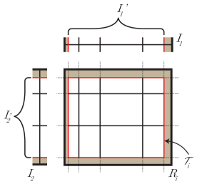
We let for intervals . We let be minus the intervals of the -partition of the coordinate that contain the endpoints of . We note that and that is a union of consecutive intervals in the partition of this coordinate. We claim that this means that is the union of at most intervals of one of the first partitions of the coordinate. This is easy to see by induction on , as is a union of consecutive intervals in the partition union at most one interval of the on either end. The one-dimensional intervals on the top and left of Figure 2 show an illustration of this.
In order to produce , we write each as a union of at most intervals from the relevant partitions. We let be the set of rectangles obtained by taking the product of one rectangle from each of these sets. It is then clear that partitions into at most pieces. Figure 2 shows an illustration of this. We now note that
Thus, satisfies all of the desired properties, and taking the union of the will yield an appropriate . This completes the proof of Lemma 2.8. ∎
3 Sample Complexity Lower Bound
In this section, we prove the sample complexity lower bound of Theorem 1.1. The structure of this section is as follows: We begin (Proposition 3.2) by providing a new proof that samples are required to test uniformity of a -histogram in one dimension. The purpose of reproving this previously known result is so that we may later generalize it to higher dimensions. We then proceed by describing a basic construction that yields a slightly improved lower bound (Proposition 3.3). Finally, we present a more sophisticated construction that suffices to establish our final lower bound in Theorem 3.4.
Basic Background.
Recall the definition of the -metric. Notice that, for fixed , is an inner product on distributions . Furthermore, by the Cauchy-Schwarz inequality it follows that if and are probability distributions then
This metric is useful for determining whether or not distributions can be distinguished. In particular, if and can be distinguished from a single sample, it must be the case that is much bigger than . Formally, we have:
Lemma 3.1.
Suppose that and are probability distributions. Suppose furthermore that there is an algorithm that given a random sample from accepts with probability at least , and given a random sample from rejects with probability at least . Then, it holds that .
Proof.
Let be the set on which the algorithm accepts. We then have that and . Therefore, we have that
∎
3.1 Lower Bound for Uniformity Testing of Univariate Histograms
We start by using Lemma 3.1 to prove a lower bound on the number of samples required to test uniformity of univariate -histograms. We build on this argument in the following subsections to establish our final multidimensional lower bound.
The idea is to use a standard adversary argument, using Lemma 3.1 to show that it is impossible to distinguish samples taken from a distribution from a particular ensemble, from those taken from the uniform distribution.
Proposition 3.2.
If there exists an algorithm that given independent samples from an unknown -histogram, , on and accepts with at least probability if and rejects with at least probability if , then .
Proof.
We assume that is even. Divide into equally sized bins. Let be a distribution over histograms where in each bin either on the first half and on the second half of the bin, or visa versa independently for each bin. Note that a sample from is always a -histogram with . Let be the distribution on obtained by randomly picking a distribution from and then taking independent samples from .
Given that an algorithm to distinguish the uniform distribution from -histograms far from it exists, such a distribution can distinguish a single sample from from a sample from . Therefore, by Lemma 3.1, we must have that We will now try to bound this quantity.
Note that is a mixture of the distributions where is drawn from . Therefore, by linearity of the -metric, we have that
where the last equality is by noting that the corresponding integral decomposes as a product.
We now need to think about the distribution of when and are drawn independently from . We note that for each bin the quantity is either or with equal probability and independently for each bin. Therefore,
where are i.i.d. random variables . Therefore,
To bound this quantity, we use the fact that, for each , the moment of a Rademacher random variable is less than or equal to the corresponding moment of the standard Gaussian. We thus have that
where the are i.i.d. random variables. We can bound this latter quantity as follows:
Hence, a testing algorithm can only exist when
or equivalently when This completes the proof of Proposition 3.2. ∎
3.2 First Attempt: Basic Multidimensional Lower Bound
In this subsection, we build on the univariate construction of the previous subsection to obtain a slightly improved lower bound in dimensions. We achieve this by modifying our ensemble in order to force any testing algorithm to guess the dimensions of the rectangles involved in the partition. Specifically, we prove the following:
Proposition 3.3.
If there exists an algorithm that, given independent samples from a -histogram, , on with , accepts with at least probability if and rejects with at least probability if , then .
Proof.
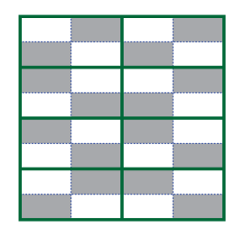
We first assume that is a power of , namely . Since this can always be achieved by decreasing by a factor of at most , this should not affect the final bound. We define an ensemble similarly to how we did so in the proof of Proposition 3.2. To define a distribution in , first we randomly and uniformly pick a -tuple of non-negative integers summing to . We call this the defining vector of . We next divide into bins by producing a grid We cut each bin into equal sub-bins by diving it in half along each dimension. We divide these sub-bins into two classes based on their parity. We then let on the sub-bins of a random parity and on the other sub-bins, where the choices are independent for each bin. We note that a drawn from is always a -histogram that is -far from the uniform distribution . An illustration is given in Figure 3.
We let be the distribution on obtained by drawing a random from and taking independent samples from . Once again, it suffices to bound from below . We similarly have that
We note that if and have the same defining vectors, then the contribution to from each bin is randomly and independently . Therefore, by the arguments of the previous subsection, if we condition on and having the same defining vectors, the expectation of is at most . On the other hand, if and have different defining vectors, we claim that . In fact, we make the stronger claim that if is the intersection of a defining bin of and a defining bin of , then . This is because without loss of generality we may assume that ’s associated is smaller than ’s associated . This in turn means that given any point in , the entire width of along the first axis will be in the same sub-bin for , but will pass through two sub-bins of opposite parity for . Thus, the average of over this line will be , and thus the integral over of is the same as the integral of .
Now since there are different possible defining vectors, we have that
In order for this to be at least , it must be the case that
or
This completes the proof of Proposition 3.3. ∎
3.3 Second Attempt: Proof of Final Sample Lower Bound
Unfortunately, the lower bound of Proposition 3.3 only saves us a factor. This is essentially because a testing algorithm only needs to correctly guess one of poly-logarithmically many defining vectors, and once it has guessed the correct one, it only needs to see a signal large enough that the probability of error is only inverse poly-logarithmic. This can be done by increasing the number of samples by only a doubly logarithmic factor. In order to do better, we will need a slightly more complicated construction, where we chop our domain into pieces and fill each piece with rectangles, but where different pieces might have rectangles of different sizes.
Theorem 3.4.
If there exists an algorithm that, given independent samples from a -histogram, , on with , accepts with at least probability if , and rejects with at least probability if , then .
Proof.
We first assume that can be written in the form , where . We note that (perhaps decreasing by a constant factor) we can achieve this with , and therefore we can assume this throughout the rest of the argument.
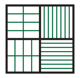
We describe a new ensemble over -histograms on in the following way: First, divide into equal volume boxes in some arbitrary way. For each box , pick a member from , the ensemble from the proof of Proposition 3.3, independently for different . We let the restriction of to be rescaled such that it assigns total mass , and such that the domain of definition is , rather than . An example element of is illustrated in Figure 4.
Similarly, it suffices to show that if is below our desired sample lower bound then
is less than .
We note that for and drawn from the quantity is distributed as with and drawn from . This is except with probability and otherwise is distributed as , where the are i.i.d. random variables. Notice that these are independent for different and sum to . Therefore,
where the are i.i.d., equal to with probability , and otherwise. Therefore, we have that
Once again, this expectation is only increased if the are replaced by standard Gaussians, and so is at most
with i.i.d. standard normals. Noting that we still have a sum of many independent Gaussians, this simplifies to
In order for this to be at least , it must be the case that
or equivalently that
This completes the proof of Theorem 3.4. ∎
Remark 3.5.
We note that our lower bounds for uniformity testing of histograms on can be made to work for histograms on , assuming that . In particular, our lower bound construction requires first dividing our domain into equal boxes, and then subdividing each of these boxes into equal boxes in such a way that the number of subdivisions in each dimension is a power of . For simplicity, let us assume that is a power of . In that case, we can first cut each edge of our original box into equal pieces and then further subdivide each side into equal pieces. We note that all of the histograms in our adversarial family are consistent with this partition of our cube into fewer than boxes. Therefore, by the inverse of the reduction above, our lower bound can be made to work on rather than . A more elaborate construction can show that our lower bounds apply for domain for any .
4 Conclusions and Future Directions
In this work, we gave a computationally efficient and sample near-optimal algorithm for the problem of testing the identity of multidimensional histogram distributions in any fixed dimension. Our nearly matching upper and lower bounds have interesting consequences regarding the relation of learning and identity testing for this important nonparametric family of distributions.
A natural direction for future work is to generalize our results to the problem of testing equivalence between two unknown multidimensional histograms. The one-dimensional version of this problem was resolved in [DKN15a, DKN17]. Additional ideas are required for this setting, as the algorithm and analysis in this work exploit the a priori knowledge of the explicit distribution.
Another direction for future work concerns characterizing the sample and computationally complexity of identity testing -dimensional -histograms when the dimension and the number of rectangles are comparable, e.g., or even . We believe that understanding these parameter regimes requires different ideas.
References
- [ADH+15] J. Acharya, I. Diakonikolas, C. Hegde, J. Li, and L. Schmidt. Fast and Near-Optimal Algorithms for Approximating Distributions by Histograms. In 34th ACM SIGMOD-SIGACT-SIGAI Symposium on Principles of Database Systems, PODS 2015, pages 249–263, 2015.
- [ADK15] J. Acharya, C. Daskalakis, and G. Kamath. Optimal testing for properties of distributions. In Advances in Neural Information Processing Systems (NIPS), pages 3591–3599, 2015.
- [ADLS16] J. Acharya, I. Diakonikolas, J. Li, and L. Schmidt. Fast algorithms for segmented regression. In Proceedings of the 33nd International Conference on Machine Learning, ICML 2016, pages 2878–2886, 2016.
- [ADLS17] J. Acharya, I. Diakonikolas, J. Li, and L. Schmidt. Sample-optimal density estimation in nearly-linear time. In Proceedings of the Twenty-Eighth Annual ACM-SIAM Symposium on Discrete Algorithms, SODA 2017, pages 1278–1289, 2017. Full version available at https://arxiv.org/abs/1506.00671.
- [BBBB72] R.E. Barlow, D.J. Bartholomew, J.M. Bremner, and H.D. Brunk. Statistical Inference under Order Restrictions. Wiley, New York, 1972.
- [BC17] T. Batu and C. L. Canonne. Generalized uniformity testing. In 58th IEEE Annual Symposium on Foundations of Computer Science, FOCS 2017, pages 880–889, 2017.
- [BCG01] N. Bruno, S. Chaudhuri, and L. Gravano. Stholes: A multidimensional workload-aware histogram. In Proceedings of the 2001 ACM SIGMOD international conference on Management of data, pages 211–222, 2001.
- [BFR+00] T. Batu, L. Fortnow, R. Rubinfeld, W. D. Smith, and P. White. Testing that distributions are close. In IEEE Symposium on Foundations of Computer Science, pages 259–269, 2000.
- [BKR04] T. Batu, R. Kumar, and R. Rubinfeld. Sublinear algorithms for testing monotone and unimodal distributions. In ACM Symposium on Theory of Computing, pages 381–390, 2004.
- [Can15] C. L. Canonne. A survey on distribution testing: Your data is big. but is it blue? Electronic Colloquium on Computational Complexity (ECCC), 22:63, 2015.
- [Can16] C. L. Canonne. Are few bins enough: Testing histogram distributions. In Proceedings of the 35th ACM SIGMOD-SIGACT-SIGAI Symposium on Principles of Database Systems, PODS 2016, pages 455–463, 2016.
- [CDGR16] C. L. Canonne, I. Diakonikolas, T. Gouleakis, and R. Rubinfeld. Testing shape restrictions of discrete distributions. In 33rd Symposium on Theoretical Aspects of Computer Science, STACS 2016, pages 25:1–25:14, 2016.
- [CDKS17a] C. L. Canonne, I. Diakonikolas, D. M. Kane, and A. Stewart. Testing bayesian networks. In Proceedings of the 30th Conference on Learning Theory, COLT 2017, pages 370–448, 2017.
- [CDKS17b] C. L. Canonne, I. Diakonikolas, D. M. Kane, and A. Stewart. Testing conditional independence of discrete distributions. CoRR, abs/1711.11560, 2017. In STOC’18.
- [CDS17] C. L. Canonne, I. Diakonikolas, and A. Stewart. Fourier-based testing for families of distributions. CoRR, abs/1706.05738, 2017. In NeurIPS 2018.
- [CDSS13] S. Chan, I. Diakonikolas, R. Servedio, and X. Sun. Learning mixtures of structured distributions over discrete domains. In SODA, pages 1380–1394, 2013.
- [CDSS14a] S. Chan, I. Diakonikolas, R. Servedio, and X. Sun. Efficient density estimation via piecewise polynomial approximation. In STOC, pages 604–613, 2014.
- [CDSS14b] S. Chan, I. Diakonikolas, R. Servedio, and X. Sun. Near-optimal density estimation in near-linear time using variable-width histograms. In NIPS, pages 1844–1852, 2014.
- [CDVV14] S. Chan, I. Diakonikolas, P. Valiant, and G. Valiant. Optimal algorithms for testing closeness of discrete distributions. In SODA, pages 1193–1203, 2014.
- [CGHJ12] G. Cormode, M. Garofalakis, P. J. Haas, and C. Jermaine. Synopses for massive data: Samples, histograms, wavelets, sketches. Found. Trends databases, 4:1–294, 2012.
- [CMN98] S. Chaudhuri, R. Motwani, and V. R. Narasayya. Random sampling for histogram construction: How much is enough? In SIGMOD Conference, pages 436–447, 1998.
- [DDK18] C. Daskalakis, N. Dikkala, and G. Kamath. Testing Ising models. In SODA, 2018.
- [DDS12] C. Daskalakis, I. Diakonikolas, and R.A. Servedio. Learning -modal distributions via testing. In SODA, pages 1371–1385, 2012.
- [DDS+13] C. Daskalakis, I. Diakonikolas, R. Servedio, G. Valiant, and P. Valiant. Testing -modal distributions: Optimal algorithms via reductions. In SODA, pages 1833–1852, 2013.
- [DGPP16] I. Diakonikolas, T. Gouleakis, J. Peebles, and E. Price. Collision-based testers are optimal for uniformity and closeness. Electronic Colloquium on Computational Complexity (ECCC), 23:178, 2016.
- [DGPP17] I. Diakonikolas, T. Gouleakis, J. Peebles, and E. Price. Sample-optimal identity testing with high probability. CoRR, abs/1708.02728, 2017. In ICALP 2018.
- [DHS15] I. Diakonikolas, M. Hardt, and L. Schmidt. Differentially private learning of structured discrete distributions. In NIPS, pages 2566–2574, 2015.
- [DK16] I. Diakonikolas and D. M. Kane. A new approach for testing properties of discrete distributions. In FOCS, pages 685–694, 2016. Full version available at abs/1601.05557.
- [DKN15a] I. Diakonikolas, D. M. Kane, and V. Nikishkin. Optimal algorithms and lower bounds for testing closeness of structured distributions. In IEEE 56th Annual Symposium on Foundations of Computer Science, FOCS 2015, pages 1183–1202, 2015.
- [DKN15b] I. Diakonikolas, D. M. Kane, and V. Nikishkin. Testing identity of structured distributions. In Proceedings of the Twenty-Sixth Annual ACM-SIAM Symposium on Discrete Algorithms, SODA 2015, pages 1841–1854, 2015.
- [DKN17] I. Diakonikolas, D. M. Kane, and V. Nikishkin. Near-optimal closeness testing of discrete histogram distributions. In 44th International Colloquium on Automata, Languages, and Programming, ICALP 2017, pages 8:1–8:15, 2017.
- [DKS16a] I. Diakonikolas, D. M. Kane, and A. Stewart. Efficient robust proper learning of log-concave distributions. CoRR, abs/1606.03077, 2016.
- [DKS16b] I. Diakonikolas, D. M. Kane, and A. Stewart. Statistical query lower bounds for robust estimation of high-dimensional gaussians and gaussian mixtures. CoRR, abs/1611.03473, 2016. In Proceedings of FOCS’17.
- [DKS18] I. Diakonikolas, D. M. Kane, and A. Stewart. Sharp bounds for generalized uniformity testing. In Advances in Neural Information Processing Systems 31, NeurIPS 2018, pages 6204–6213, 2018.
- [DL04] L. Devroye and G. Lugosi. Bin width selection in multivariate histograms by the combinatorial method. Test, 13(1):129–145, 2004.
- [DLS18] I. Diakonikolas, J. Li, and L. Schmidt. Fast and sample near-optimal algorithms for learning multidimensional histograms. In Sébastien Bubeck, Vianney Perchet, and Philippe Rigollet, editors, Proceedings of the 31st Conference On Learning Theory, volume 75 of Proceedings of Machine Learning Research, pages 819–842. PMLR, 2018.
- [DP17] C. Daskalakis and Q. Pan. Square Hellinger subadditivity for Bayesian networks and its applications to identity testing. In Proceedings of the 30th Conference on Learning Theory, COLT 2017, pages 697–703, 2017.
- [FD81] D. Freedman and P. Diaconis. On the histogram as a density estimator:l2 theory. Zeitschrift für Wahrscheinlichkeitstheorie und Verwandte Gebiete, 57(4):453–476, 1981.
- [GGI+02] A. C. Gilbert, S. Guha, P. Indyk, Y. Kotidis, S. Muthukrishnan, and M. Strauss. Fast, small-space algorithms for approximate histogram maintenance. In STOC, pages 389–398, 2002.
- [GGR98] O. Goldreich, S. Goldwasser, and D. Ron. Property testing and its connection to learning and approximation. Journal of the ACM, 45:653–750, 1998.
- [GJ14] P. Groeneboom and G. Jongbloed. Nonparametric Estimation under Shape Constraints: Estimators, Algorithms and Asymptotics. Cambridge University Press, 2014.
- [GKS06] S. Guha, N. Koudas, and K. Shim. Approximation and streaming algorithms for histogram construction problems. ACM Trans. Database Syst., 31(1):396–438, 2006.
- [GKTD00] D. Gunopulos, G. Kollios, V. J. Tsotras, and C. Domeniconi. Approximating multi-dimensional aggregate range queries over real attributes. In Proceedings of the 2000 ACM SIGMOD International Conference on Management of Data, pages 463–474, 2000.
- [Gol17] O. Goldreich. Introduction to Property Testing. Forthcoming, 2017.
- [Gre56] U. Grenander. On the theory of mortality measurement. Skand. Aktuarietidskr., 39:125–153, 1956.
- [ILR12] P. Indyk, R. Levi, and R. Rubinfeld. Approximating and Testing -Histogram Distributions in Sub-linear Time. In PODS, pages 15–22, 2012.
- [JKM+98] H. V. Jagadish, N. Koudas, S. Muthukrishnan, V. Poosala, K. C. Sevcik, and T. Suel. Optimal histograms with quality guarantees. In VLDB, pages 275–286, 1998.
- [Kle09] J. Klemela. Multivariate histograms with data-dependent partitions. Statistica Sinica, 19(1):159–176, 2009.
- [LN96] G. Lugosi and A. Nobel. Consistency of data-driven histogram methods for density estimation and classification. Ann. Statist., 24(2):687–706, 04 1996.
- [Mut05] S. Muthukrishnan. Data streams: Algorithms and applications. Found. Trends Theor. Comput. Sci., 1(2):117–236, 2005.
- [NP33] J. Neyman and E. S. Pearson. On the problem of the most efficient tests of statistical hypotheses. Philosophical Transactions of the Royal Society of London. Series A, Containing Papers of a Mathematical or Physical Character, 231(694-706):289–337, 1933.
- [Pan08] L. Paninski. A coincidence-based test for uniformity given very sparsely-sampled discrete data. IEEE Transactions on Information Theory, 54:4750–4755, 2008.
- [Pea00] K. Pearson. On the criterion that a given system of deviations from the probable in the case of a correlated system of variables is such that it can be reasonably supposed to have arisen from random sampling. Philosophical Magazine Series 5, 50(302):157–175, 1900.
- [PI97] V. Poosala and Y. E. Ioannidis. Selectivity estimation without the attribute value independence assumption. In Proceedings of the 23rd International Conference on Very Large Data Bases, VLDB ’97, pages 486–495, San Francisco, CA, USA, 1997. Morgan Kaufmann Publishers Inc.
- [RS96] R. Rubinfeld and M. Sudan. Robust characterizations of polynomials with applications to program testing. SIAM J. on Comput., 25:252–271, 1996.
- [Rub12] R. Rubinfeld. Taming big probability distributions. XRDS, 19(1):24–28, 2012.
- [Sco79] D. W. Scott. On optimal and data-based histograms. Biometrika, 66(3):605–610, 1979.
- [Sco92] D.W. Scott. Multivariate Density Estimation: Theory, Practice and Visualization. Wiley, New York, 1992.
- [TGIK02] N. Thaper, S. Guha, P. Indyk, and N. Koudas. Dynamic multidimensional histograms. In SIGMOD Conference, pages 428–439, 2002.
- [VV14] G. Valiant and P. Valiant. An automatic inequality prover and instance optimal identity testing. In FOCS, 2014.
- [WN07] R. Willett and R. D. Nowak. Multiscale poisson intensity and density estimation. IEEE Transactions on Information Theory, 53(9):3171–3187, 2007.
Appendix
Appendix A Proof of Theorem 2.3
We use the flattening method developed in [DK16]. We begin by giving the definition of a split distribution from that work:
Definition A.1.
Given a distribution on and a multiset of elements of , define the split distribution on as follows: For , let denote plus the number of elements of that are equal to . Thus, We can therefore associate the elements of to elements of the set . We now define a distribution with support , by letting a random sample from be given by , where is drawn randomly from and is drawn randomly from .
We recall a basic fact about split distributions:
Fact A.2 (Fact 2.5, [DK16]).
Let and be probability distributions on , and be a given multiset of . Then: (i) We can simulate a sample from or by taking a single sample from or , respectively. (ii) It holds .
We also recall an optimal -closeness tester under the promise that one of the distributions has small -norm:
Lemma A.3 ([CDVV14]).
Let and be two unknown distributions on . There exists an algorithm that on input , and , draws samples from each of and and, with probability at least , distinguishes between the cases that and
We now have all the necessary tools to describe and analyze our -identity tester. The pseudo-code of our algorithm follows:
Input: sample access to discrete distribution , , and ,
and explicit distribution .
Output: “YES” if ; “NO” if
-
1.
Let be the multiset obtained by taking copies of .
-
2.
Use the -tester of Lemma A.3 to distinguish between the cases that and and return the result.
We now provide the simple analysis. Note that and that assigns probability mass at most to each domain element. Therefore, we have that By Lemma A.3 — applied for and in place of — we obtain that the -tester in Step 2 of the above pseudo-code requires samples from and . Since is explicitly given, so is and therefore we can straightforwardly generate samples from for free. By Fact A.2, we can generate a sample from given a sample from . Hence, our algorithm uses samples from . This completes the analysis of the sample complexity.
We now prove correctness. If , then by Fact A.2 we have that and the algorithm will return “YES” with appropriate probability. On the other hand, if , then by definition of the metric it follows that , for . Since elements contribute to total -error at least , by the Cauchy-Schwarz inequality, we have that
where we used the fact that . Therefore, in this case, the algorithm returns “NO” with appropriate probability. This completes the proof of Theorem 2.3.