A Model of Sunspot Number with Modified Logistic Function

Abstract

Solar cycles are studied with the Version 2 monthly smoothed international sunspot number, the variations of which are found to be well represented by the modified logistic differential equation with four parameters: maximum cumulative sunspot number or total sunspot number $x_{m}$, initial cumulative sunspot number $x_{0}$, maximum emergence rate $r_{0}$, and asymmetry $\alpha$. A two-parameter function is obtained by taking $\alpha$ and $r_{0}$ as fixed value. In addition, it is found that $x_{m}$ and $x_{0}$ can be well determined at the start of a cycle. Therefore, a prediction model of sunspot number is established based on the two-parameter function. The prediction for cycles $4-23$ shows that the solar maximum can be predicted with average relative error being 8.8% and maximum relative error being 22% in cycle 15 at the start of solar cycles if solar minima are already known. The quasi-online method for determining solar minimum moment shows that we can obtain the solar minimum 14 months after the start of a cycle. Besides, our model can predict the cycle length with the average relative error being 9.5% and maximum relative error being 22% in cycle 4. Furthermore, we predict the sunspot number variations of cycle 24 with the relative errors of the solar maximum and ascent time being 1.4% and 12%, respectively, and the predicted cycle length is 11.0 (95% confidence interval is 8.3$-$12.9) years. The comparison to the observation of cycle 24 shows that our prediction model has good effectiveness.

1 Introduction

Sunspot number is a good indicator of solar activity and its change follows an 11-year cycle. Solar activity has influence on the galactic cosmic ray intensity (e.g., McDonald, 1998; Qin & Shen, 2017; Shen & Qin, 2018) that has impact on the health of astronauts and safety of spacecraft. It is also suggested that solar activity may affect Earth’s climate (e.g., Haigh, 2007). There is evidence that the energy spectrum of ground-level enhancement (GLE) of solar energetic particle events is relevant with the 10.7 cm solar radio flux (Wu & Qin, 2018) that is highly correlated with sunspot number (e.g., Holland & Vaughan, 1984; Hathaway, 2015), so that the prediction of the time profile of sunspot number is helpful for estimating the spectra of potential GLEs. In addition, the fact that sunspot number is related to other solar parameters may guide us to better understand the origin of solar cycles.

In order to describe the variations of sunspot number in one solar cycle, Stewart & Panofsky (1938) adopted Pearson’s Type III distribution function with a power law for the rising phase and an exponential for the decline phase. Furthermore, Hathaway et al. (1994) constructed a quasi-Planck function similar to that of Stewart & Panofsky (1938) but with a fixed (cubic) power law for the rising phase and a Gaussian for the decline phase, which is given by (Hathaway et al., 1994; Hathaway, 2015):

$$f\left(t\right)=a\left(t-t_{0}\right)^{3}\left[\exp{\left(\frac{t-t_{0}}{b}\right)^{2}}-c\right]^{-1}$$ (1)

with four parameters, namely, amplitude $a$, starting time $t_{0}$, rise time $b$, and asymmetry $c$. They found that the asymmetry $c$ can be taken as a fixed value and the rise time $b$ is relevant with the amplitude $a$, so that the function could be reduced to a two-parameter form and the sunspot number could still be fitted well. They found that the amplitude can be estimated at the start of a solar cycle by using the correlation between the amplitude and the length of the previous cycle, and the relative error is within about 30%. At some time $\Delta t$ that a solar cycle has progressed one can use this model to fit the observed data and thus one can predict the sunspot number for the rest of the cycle. They concluded that the accuracy of the predicted amplitude is within about $20$% and $10$% if $\Delta t=30$ and $42$ months, respectively. Volobuev (2009) suggested a function that is similar to Maxwell distribution with three parameters to represent the sunspot number (e.g., Roshchina & Sarychev, 2011), and they also obtained a two-parameter form by reducing one of the parameters. Note that, they considered it to be one-parameter fit because the parameter of starting time was neglected to fit. They found that the fitting effects of their model were similar to that of Hathaway et al. (1994). What’s more, they concluded that their empirical model did better than dynamo ones in fitting the sunspot number. By introducing an asymmetry factor $\alpha$ to describe the asymmetry of the sunspot number during a solar cycle, Du (2011) introduced a modified Gaussian function

$$f\left(t\right)=A\exp{\left(\frac{-\left(t-t_{m}\right)^{2}}{2B^{2}\left[1+\alpha\left(t-t_{m}\right)\right]^{2}}\right)}$$ (2)

with four parameters, among which they found that $B$ and $\alpha$ can be obtained by quadratic functions of $t_{m}$, and thus the number of parameters is reduced to two. Based on the two-parameter function, they concluded that the accuracy of predicted maximum sunspot number is within $15$% if $\Delta t=25$ months.

Gnevyshev (1963) found that during solar maximum sunspot number usually has double-peak with a gap in between, which is called Gnevyshev gap. In order to fit this phenomenon Sabarinath & Anilkumar (2008) suggested the modified binary mixture of the Laplace distribution functions

$$f\left(t\right)=\frac{A_{1}}{2S_{1}}\exp{\left(\frac{-|t-M_{1}|}{S_{1}}\right)}+\frac{A_{2}}{2S_{2}}\exp{\left(\frac{-|t-M_{2}|}{S_{2}}\right)}$$ (3)

with six parameters as the model of sunspot number. They also obtained a two-parameter function by using empirical values for $M_{1}$, $M_{2}$, $S_{1}$, and $S_{2}$. Recently, Li et al. (2017) proposed a simplified binary mixture of Gaussian functions as follows:

$$f\left(t\right)=A_{1}\exp{\left(\frac{-\left(t-M_{1}\right)^{2}}{S_{1}}\right)}+A_{2}\exp{\left(\frac{-\left(t-M_{2}\right)^{2}}{S_{2}}\right)}$$ (4)

with six parameters too, which, however, shows better results in the double-peak to fit monthly smoothed sunspot number data. In addition, they found that the function could be reduced to a three-parameter form since the parameters $M_{2}$, $S_{1}$, and $A_{2}$ could be represented by $M_{1}$.

It is shown that empirical functions can be used to represent the variations of sunspot number during a solar cycle with demonstrated prediction power, but they usually do not obtain a good prediction result for a solar cycle until 2 to 3 years that the solar cycle has progressed, i.e., $\Delta t=2$ to $3$ years (Hathaway et al., 1994; Du, 2011; Hathaway, 2015). In this paper we use the modified logistic differential equation to reproduce the variations of sunspot number during solar cycles, and thus a prediction model is established with good effectiveness. In section 2, sunspot data are presented. In section 3, our new sunspot number model with modified logistic function is presented. In section 4, we show the results of the new model. In section 5, the prediction ability of our model is presented. And conclusions are presented in section 6.

2 Sunspot data

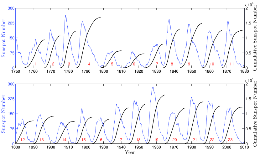
Figure 1: Blue and black curves are monthly smoothed sunspot number and cumulative sunspot number, respectively, for cycles $1-23$. The numbers in the figure indicate the cycle number.

In this work, we use the Versions 1 and 2 (Clette et al., 2015) monthly and monthly smoothed international sunspot number, which can be downloaded from http://www.sidc.be/silso/. Monthly smoothed sunspot number, which is obtained by using the standard smoothing with a 13-month running mean centered on the month of interest with half weights for the months at the start and end (e.g., Hathaway, 2015), is adopted to study the shape of solar cycles. The solar maximum is obtained by taking the mathematical maximum of the monthly smoothed sunspot number in a solar cycle, and the solar minimum is obtained by taking the mathematical minimum of the monthly smoothed sunspot number in the period from the previous solar maximum to current one. Note that, if the minimum/maximum value is occurred more than once in a period, the first occurrence is taken as the epoch of the minimum/maximum (e.g., Kakad, 2011). For example, the minimum value between the solar maximum epoch of cycle 22 and that of cycle 23 is 11.2 that occurred in May 1996 and August 1996, we choose May 1996 as the solar minimum epoch of solar cycle 23. The blue and black curves in Figure 1 represent monthly smoothed sunspot numbers of Version 2 and their cumulative values for solar cycles, respectively. In other words, the blue curves are the time derivative of the black ones.

3 Sunspot number model with modified logistic function

3.1 Logistic function

Logistic function is proposed by Verhulst (1838) for modeling population growth, and the function has been successfully used in many fields such as statistics, machine learning, chemistry, physics, economics, and sociology. In the model, the growth of population is related to the number of the current population, which can be written as:

$$\frac{dx}{dt}=rx,$$ (5)

where $x$ and $r$ are the current population and growth rate, respectively. Due to the limitation of environmental factors, the growth rate decreases with the increase of population, which has a maximum value $x_{m}$. Consequently, the growth rate $r$ can be written as:

$$r(x)=r_{0}-kx,$$ (6)

where $r_{0}$ and $k$ are constants with $r_{0}$ being called intrinsic growth rate. When the population reaches its maximum value $x_{m}$, the growth rate $r$ becomes zero, i.e., $r(x_{m})=0$. Therefore, the constant $k$ could be eliminated, and Equation (6) is rewritten as:

$$r(x)=r_{0}\left(1-\frac{x}{x_{m}}\right).$$ (7)

Substituting Equation (7) into Equation (5), the differential equation of population is given by:

$$\frac{dx}{dt}=r_{0}\left(1-\frac{x}{x_{m}}\right)x.$$ (8)

Using the initial condition $x|_{t=0}=x_{0}$, the integral equation of population is derived as:

$$x\left(t\right)=x_{m}\left[1+\left(\frac{x_{m}}{x_{0}}-1\right)e^{-r_{0}t}\right]^{-1},$$ (9)

which is called logistic function.

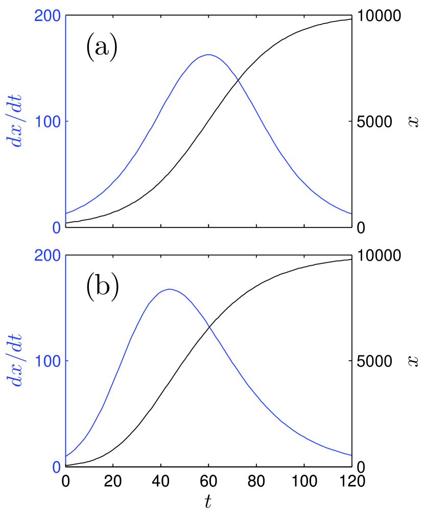
Figure 2: (a) Black and blue curves are logistic function and its derivative, respectively, with $x_{0}$=200, $r_{0}$=0.065, and $x_{m}$=10000. (b) Same as Panel (a) but for modified logistic model with $\alpha=0.2$, $x_{0}$=60, $r_{0}$=0.25, and $x_{m}$=10000.

In Figure 2(a), the black curve shows the logistic function, and the blue curve is the derivative of the black one. It can be seen that the black curve in Figure 2(a) (logistic function) is similar to the black curve in Figure 1 (cumulative sunspot numbers), so that one may use the logistic model to study the variations of solar cycles. However, the shape of logistic differential equation (Equation 8) in Figure 2(a) is symmetrical about its peak, while the shape of solar cycles is usually asymmetrical about its peak. Therefore, the logistic function needs to be modified to show asymmetry.

3.2 Modified logistic function

In order to obtain an asymmetrical logistic differential equation, we replace $x$ with $x^{\alpha}$ in Equation (6) to get:

$$r(x)=r_{0}-kx^{\alpha},$$ (10)

where $\alpha$ is a positive constant. It is noted that in the new Equation (10) the relationship between $r$ and $x$ is no longer linear. The modified differential and integral equations corresponding to Equations (8) and (9) are derived as:

$$\frac{dx}{dt} = r_{0}\left(1-\frac{x^{\alpha}}{x_{m}^{\alpha}}\right)x,$$ (11)

$$x\left(t\right) = x_{m}{\left[1+\left(\frac{x_{m}^{\alpha}}{x_{0}^{\alpha}}-1\right)e^{-\alpha r_{0}t}\right]^{-1/\alpha}},$$ (12)

which is very similar to the generalized logistic function (Richards, 1959; Birch, 1999; Balakrishnan, 2010). In Figure 2(b), the black and blue curves show the modified logistic function and its differential results with $\alpha=0.2$, respectively. We can see that the blue curve shows asymmetry about its peak, i.e., it increases rapidly before the peak while decreases slowly after the peak.

3.3 Models of sunspot number

The Equations (8) and (11) could be rewritten as follows:

$$f\left(x\right) = r_{0}\frac{x}{x_{m}}\left(x_{m}-x\right)=r_{0}\frac{x}{x_{m}}x_{r},$$ (13)

$$f\left(x\right) = r_{0}\frac{x}{x_{m}}\frac{x_{m}^{\alpha}-x^{\alpha}}{x_{m}^{\alpha-1}}=r_{0}\frac{x}{x_{m}}x_{r}^{\prime},$$ (14)

where $dx/dt$ is replaced with $f$ that denotes the sunspot number. The parameters $x$ and $x_{m}$ represent current population and maximum population, respectively, in Ecology. However, in this work we call $x$ and $x_{m}$ as the current cumulative sunspot number and maximum cumulative sunspot number or total sunspot number of a solar cycle. Thus, the term $x_{r}=x_{m}-x$ in Equation (13) indicates the residual sunspot number, which changes from $x_{m}$ to zero. In other words, the remaining sunspot number that the Sun will produce in the solar cycle is $x_{r}=x_{m}-x$. In the modified Equation (14), the term $x_{r}=x_{m}-x$ in Equation (13) is modified as $x_{r}^{\prime}=\left(x_{m}^{\alpha}-x^{\alpha}\right)/x_{m}^{\alpha-1}$, which also changes from $x_{m}$ to zero. Thus the term $x_{r}^{\prime}$ represents the modified residual sunspot number. With the definition of $x_{r}=x_{m}-x$, the term $r_{0}\left(x/x_{m}\right)$ could be called as emergence rate of sunspot which changes from zero to $r_{0}$, so that $r_{0}$ indicates the maximum emergence rate of sunspot. In addition, the parameters $x_{0}$ and $\alpha$ can be called initial cumulative sunspot number and asymmetry, respectively. Finally, the cumulative sunspot number $x\left(t_{e}\right)$ at the end of solar cycle $t_{e}$ expressed by Equation (12) is indicated by $x_{e}$. Note that the variable $t$ in Equation (12) represents the months that a solar cycle has progressed. Thus, we obtain the model of sunspot number with a modified logistic differential equation expressed with Equation (14).

4 Results

4.1 Fitting results

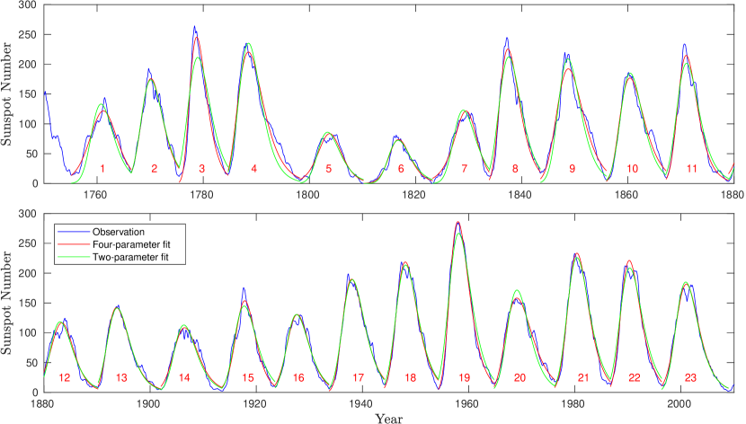
Figure 3: Monthly smoothed sunspot number curve (blue) and the fitting results by the four-parameter modified logistic differential equation (red) and the two-parameter modified logistic differential equation (green), for cycles $1-23$.

We fit the Version 2 monthly smoothed sunspot number data with the model from the modified logistic differential equation for solar cycles from $1$ to $23$, using the non-linear least squares technique based on BFGS algorithm that is an iterative method for solving unconstrained nonlinear optimization problems (Fletcher, 1987) to optimize the free parameters. In this work, the initial values of $\alpha$ and $r_{0}$ are all set to 0.2, and that of $x_{m}$ is set to the observed total sunspot numbers of a cycle. Besides, the initial value of $x_{0}$ can be obtained by combining Equation (14) with the conditions $x|_{t=0}=x_{0}$ and $f(x_{0})=S_{0}$, which is the monthly smoothed sunspot number of the first month of a cycle. Based on the configuration of the initial values, the fitting shows good stability and convergence can be achieved for all of the cycles. The red curves in Figure 3 exhibit the fitting results, and the blue curves are the observations. From the figure we can see that the model can fit sunspot number data very well. The four fitting parameters $\alpha$, $r_{0}$, $x_{0}$, and $x_{m}$ with their uncertainties and the value $x_{e}$ are shown in Table 1.

4.2 Evaluating of the fitting results

In order to evaluate the fitting results, we calculate the fitting deviation $\sigma$ (Li, 1999)

$$\sigma=\sqrt{\frac{\sum_{i=1}^{N}\left(S_{i}-f_{i}\right)^{2}}{N}},$$ (15)

and the correlation coefficient $CC$ (Bevington & Robinson, 2003)

$$CC=\sqrt{1-\frac{\sum_{i=1}^{N}\left(S_{i}-f_{i}\right)^{2}}{\sum_{i=1}^{N}\left(S_{i}-\overline{S}\right)^{2}}},$$ (16)

where $S_{i}$ and $f_{i}$ represent observed and fitted sunspot numbers, respectively. Besides, we use the Anderson-Darling distance $A^{2}$ that is the basis of Anderson-Darling test to measure the goodness-of-fit,

$$A^{2}=n\int_{-\infty}^{\infty}\frac{\left(F_{n}\left(t\right)-F\left(t\right)\right)^{2}}{F\left(t\right)\left(1-F\left(t\right)\right)}dF\left(t\right),$$ (17)

where $F$ is the theoretical distribution and $F_{n}$ is the empirically observed distribution. Equation (17) shows that the Anderson-Darling distance $A^{2}$ places more weight on observations in the tails of the distribution. The procedure we calculate $A^{2}$ is as follows: Firstly, we should consider the curve of sunspot numbers as a distribution, i.e., the months $t_{i}$ from the beginning of a solar cycle is an observed sample value and $S_{i}$ or $f_{i}$ is the number of sample $t_{i}$. Secondly, we calculate the cumulative distribution function $\Phi$ according to the fitted curve. Lastly, we use the discrete formula to calculate the Anderson-Darling distance

$$A^{2}=-n-\sum\limits_{j=1}^{n}\frac{2j-1}{n}\left[\ln{\left(\Phi\left(Y_{j}\right)\right)}+\ln{\left(1-\Phi\left(Y_{n+1-j}\right)\right)}\right].$$ (18)

Here, $Y$ denotes sample value and $n$ is the total number of samples.

The results of evaluating indices, $A^{2}$, $\sigma$, and $CC$, are also listed in Table 1.

4.3 Features of solar cycles

For a solar cycle, the most important features are the cycle length $T_{c}$, the ascent time $T_{a}$, the descent time $T_{d}$, the solar maximum $S_{m}$, and the solar minimum $S_{0}$. In the following, we give the expressions of the features about the four logistic parameters. Note that the units of $T_{c}$, $T_{a}$, and $T_{d}$ are years.

Firstly, $S_{m}$ and $T_{a}$ can be derived by solving the equation $df/dt=0$,

$$S_{m} = \frac{\alpha}{1+\alpha}\left(\frac{1}{1+\alpha}\right)^{1/\alpha}r_{0}x_{m},$$ (19)

$$T_{a} = \left(12\alpha r_{0}\right)^{-1}\ln{\frac{x_{m}^{\alpha}/x_{0}^{\alpha}-1}{\alpha}}.$$ (20)

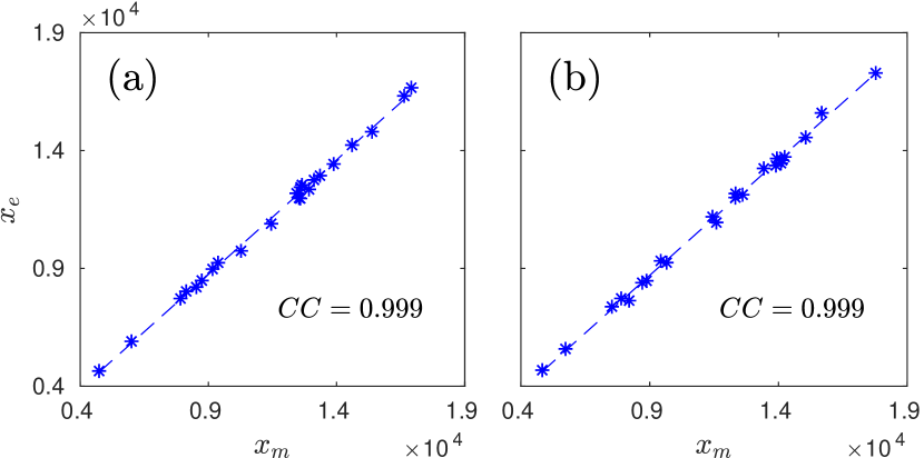
Figure 4: $x_{e}$ as a function of $x_{m}$. Dashed line indicates the linear fitting between $x_{e}$ and $x_{m}$ with correlation coefficient $CC=0.999$. Panels (a) and (b) show the fitting results with the sunspot number models of four- and two-parameter modified logistic differential equation, respectively.

Secondly, when a cycle reaches its end, the variables $t$ and $x$ in Equation (12) becomes $t_{e}$ and $x_{e}$, respectively, where $x_{e}$ is the fitted cumulative sunspot number at the end of the cycle, and thus we can obtain the value of $t_{e}$ if $x_{e}$ is already known. Figure 4(a) shows the relationship between the parameters $x_{e}$ and $x_{m}$ for solar cycles 1$-$23. The linear fitting is shown as a dashed line

$$x_{e}=0.9722x_{m}-6.93$$ (21)

with correlation coefficient $CC=0.999$ and significant at nearly 100% confidence level. Therefore, $x_{e}$ can be estimated by the linear Equation (21), and $T_{c}$ can be expressed as:

$$T_{c}\equiv\frac{t_{e}}{12}=\left(12\alpha r_{0}\right)^{-1}\ln{\frac{x_{m}^{\alpha}/x_{0}^{\alpha}-1}{x_{m}^{\alpha}/x_{e}^{\alpha}-1}}.$$ (22)

Thirdly, $T_{d}$ can be obtained by subtracting $T_{a}$ from $T_{c}$,

$$T_{d}=\left(12\alpha r_{0}\right)^{-1}\ln{\frac{\alpha}{x_{m}^{\alpha}/x_{e}^{\alpha}-1}}.$$ (23)

Lastly, combining the initial condition $x|_{t=0}=x_{0}$ with Equation (14), $S_{0}$ can be presented as:

$$S_{0}=r_{0}\frac{x_{0}}{x_{m}}\frac{x_{m}^{\alpha}-x_{0}^{\alpha}}{x_{m}^{\alpha-1}}.$$ (24)

So that, if we have the fitting results of the four logistic parameters, we can get the feature parameters of the solar cycles as shown above. The absolute relative errors of $S_{m}$ and $T_{a}$ are listed in Table 1, it can be seen that the relative error is generally in low level.

4.4 Two-parameter function

The variances and covariances denoted as $\sigma_{ij}$ $(i,j=\alpha,r_{0},x_{0},x_{m})$ of the best fit parameter values are also presented in Table 1. We can see that the covariance between parameters $\alpha$ and $r_{0}$ are large (negative) relative to their variances for all of the cycles. Thus, an increase in $\alpha$ could lead to a decrease in $r_{0}$ without changing the overall quality of the fit substantially, which makes the parameters hard to interpret. Besides, the covariance between parameters $\alpha$ and $x_{0}$ are also large relative to their variances for some cycles. Therefore, the parameter $\alpha$ should be eliminated.

From Table 1 we can see that for the fitting results the mean and standard deviation of the asymmetry $\alpha$ are 0.317 and 0.339, respectively, and the mean and standard deviation of the maximum emergence rate $r_{0}$ are 0.479 and 0.480, respectively. Though for solar cycles $1-23$, $\alpha$ ranges from 0.0274 to 1.28, we find that the fitting results are also very good if a suitable fixed value of $\alpha$ is chosen for all of the cycles. Next, we set $\alpha$ as a constant $0.2$ and a three-parameter function is obtained. After fitting the three-parameter function to the sunspot number data of solar cycles $1-23$, we get the mean and standard deviation of $r_{0}$ as 0.224 and 0.029, respectively, which indicates that the new model is more stable than the four-parameter one. Therefore, $r_{0}$ could be fixed to 0.224 for all of the cycles. Therefore, the four-parameter modified logistic function is reduced to a two-parameter one as

$$f\left(x\right) = 0.224\frac{x}{x_{m}}\frac{x_{m}^{0.2}-x^{0.2}}{x_{m}^{-0.8}}$$ (25)

$$x\left(t\right) = x_{m}{\left[1+\left(\frac{x_{m}^{0.2}}{x_{0}^{0.2}}-1\right)e^{-0.0448t}\right]^{-5}}.$$ (26)

We fit the two-parameter modified logistic differential equation to the sunspot number data of solar cycles $1-23$, the results are exhibited by the green curves in Figure 3. It is shown that the two-parameter function can fit sunspot number data very well. Figure 4(b) shows the relationship between the parameters $x_{e}$ and $x_{m}$ fitted by the two-parameter function for solar cycles 1$-$23. The linear fitting is shown as a dashed line

$$x_{e}=0.9778x_{m}-95.46$$ (27)

with correlation coefficient $CC=0.999$ and significant at nearly 100% confidence level. Therefore, with two-parameter function, $T_{c}$ can also be estimated by Equations (22) and (27). The fitting parameters and their uncertainties, the evaluating indices, and the absolute relative errors of $S_{m}$ and $T_{a}$ are listed in Table 2. It can be seen that the fitting results of two-parameter function is similar to that of four-parameter one, so that the two-parameter function is also suitable for representing the sunspot number variations of solar cycles. Table 2 also presented the variances and covariances of the two best fit parameter values, and we can find that the covariance $\sigma_{x_{0}x_{m}}$ is small for all of the cycles.

A model with less parameters is beneficial for prediction. On the one hand, when a solar cycle has progressed for 2 to 3 years, i.e., $\Delta t=2$ to 3 years, some models can be used to fit the data available to predict the behaviour of the remaining cycle (e.g., Du, 2011; Hathaway, 2015). In general, the model with fewer parameters would obtain better prediction results if there are less data available to fit. On the other hand, if we want to predict the sunspot number variations at the start of a solar cycle, only very few parameters can be estimated. Therefore, to reduce to two parameters is important for us to construct the prediction model based on the modified logistic differential equation.

4.5 Comparison of fitting effects with other functions

Schwarz (1978) proposed the index $BIC$, the Bayesian information criterion or Schwarz criterion, with the lower value preferred, to establish whether one model is significantly better than another,

$$BIC=\ln{\left(N\right)}k-2\ln{\hat{\left(L\right)}},$$ (28)

where $N$ is the number of months in a cycle while $k$ and $\hat{L}$ are the number of parameters and value of the likelihood function of a model, respectively.

Table 3 illustrates the fitting effects of three kinds of modified logistic differential equations, quasi-Plank function Equation (1), and modified Gaussian function Equation (2) for fitting Versions 1 and 2 sunspot number from cycles 1 to 23. Column 7 of Table 3 shows the average of $BIC$.

Table 3 shows that the fitting effects of four-parameter modified logistic differential equation are similar with those of four-parameter modified Gaussian function, and the performance of three-parameter modified logistic differential equation is similar with that of three-parameter quasi-Plank function. In fact, the difference between the fitting results of the five models is not significant.

5 Prediction ability

5.1 Prediction model

In order to use the two-parameter function to predict the variations of sunspot numbers, we have to estimate the two parameters, i.e., $x_{0}$ and $x_{m}$.

For estimating $x_{m}$, we use Shannon entropy (also named as information entropy) as the potential predictor. Shannon entropy is proposed by Shannon (Shannon, 1948) last century and applied to space physics recently (e.g., Laurenza et al., 2012; Qin & Zhao, 2013; Kakad et al., 2015, 2017a). It is a commonly used quantity to characterize the inherent randomness in the system. Kakad et al. (2017a) divided every solar cycle to 5 phases each of which had an equal length of $T_{c}/5$, then they calculated the value of Shannon entropy for each phase using daily sunspot number. Based on the Shannon entropy, they predicted the maximum sunspot numbers for solar cycle 25. We follow Kakad et al. 2017a to calculate the Shannon entropy. However, we use monthly sunspot number instead of daily one so that the calculation can be extended before solar cycle 10. The Shannon entropy values calculated by Version 2 sunspot number are listed in Table 4 for cycles $1-23$, in which the Shannon entropy values are denoted as $E_{i}$ where $i=1-5$ denoting the phase number. The table also includes the data $T_{c}$ in the last column. Due to the fact that $S_{m}$ is highly correlated with $x_{m}$ ($r=0.97$ and significant at nearly 100% confidence level for two-parameter fitting results) and the fact that $S_{m}$ is inversely proportional to the length of the previous cycle (Hathaway et al., 1994), we use $E_{i}^{n-3}$, $E_{i}^{n-2}$, $E_{i}^{n-1}$, and $T_{c}^{n-1}$ as potential predictors to estimate $x_{m}^{n}$. Here the superscript denotes the cycle number. The stepwise regression method is used to deal with the multi-variable linear regression. We find that $x_{m}^{n}$ can be expressed as:

$$x_{m}^{n}=g^{n} \equiv -3509E_{4}^{n-3}+3097E_{2}^{n-2}+4327E_{5}^{n-2}-3190E_{1}^{n-1}$$ (29)

$$+3189E_{4}^{n-1}+1397E_{5}^{n-1}-624T_{c}^{n-1}-11862.$$

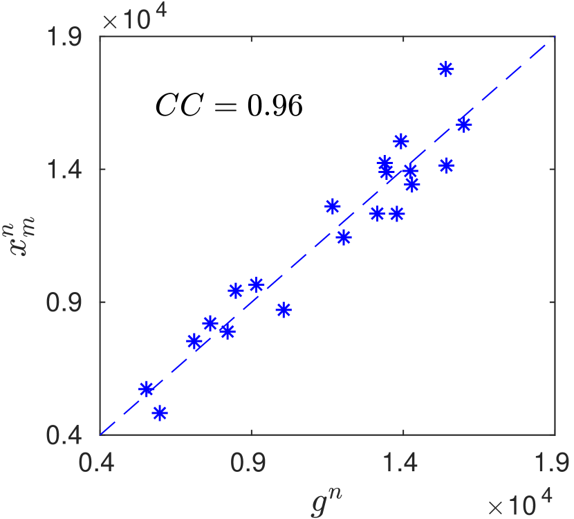
Figure 5: Parameter $x_{m}$ as a function of $g^{n}$ which depends on the Shannon entropy values of the previous three cycles and the length of last cycle. Here, $n$ denotes cycle number.

Figure 5 shows the relationship between the fitted value of $x_{m}^{n}$ and $g^{n}$ from linear equation (29). The dashed line indicates the linear fitting between $x_{m}$ and $g^{n}$ with the correlation coefficient being $0.96$ and significant at nearly 100% confidence level. Note that $g^{n}$ depends on the Shannon entropy in solar cycles $n-3$, $n-2$, and $n-1$, and $T_{c}$ in solar cycle $n-1$. Therefore, $x_{m}$ can be predicted at the start of the cycle.

The other parameter $x_{0}$ can be solved by taking the known quantities $S_{0}$, which is the sunspot number of the first month, i.e., solar minimum, and $x_{m}$ into Equation (24). Note that, the value of $S_{0}$ of cycle 6 is 0, thus the corresponding $x_{0}$ is also equals to 0, causing the sunspot number not to growth according to Equation (11). Therefore, $S_{0}$ of cycle 6 is assigned a value of 0.2, which is the minimum observed value except $0$ for all of the cycles. So that the sunspot number variations of a solar cycle can be predicted at the start of the cycle. The prediction model in this work is denoted as TMLP (Two-parameter Modified Logistic Prediction) model, hereafter.

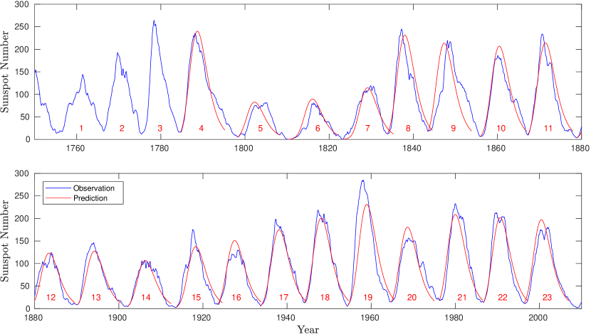
Figure 6: Blue curves are the monthly smoothed sunspot number for cycles $1-23$, and the red curves are the TMLP predicting results based on the two-parameter modified logistic differential equation for cycles $4-23$.

Figure 6 shows the prediction results by TMLP for Version 2 sunspot number from cycles $4-23$. The predicted cycle lengths are calculated by Equation (22). The evaluating indices and the absolute relative error of $S_{m}$, $T_{a}$, and $T_{c}$ are exhibited in Table 5. It is noted that to calculate the evaluating indices with Equations (15$-$17) the cycle length has to be correct, so the observed cycle length is used. From Figure 6 and Table 5 we can see that the prediction results are good except for cycles 5, 9, and 19. The average relative error of $S_{m}$ is 8.8% and the maximum one is 22% in cycle 15. For $T_{a}$, the average relative error is 17% and the maximum one is 71% in cycle 5, during which the sunspot number increases in the beginning but decreases after about 1 year. If solar cycle 5 is removed the average relative error of $T_{a}$ is 14%. The average relative error of $T_{c}$, which is not predicted by other fitting functions in the literature, is 9.5%.

5.2 Quasi-online determination of solar minimum moment

The above prediction is based on the condition that the solar minimum of a new cycle is already known, and thus the moment of solar minimum needs to be determined by using a quasi-online method. In fact, the goodness of prediction result strongly depends on the accurate determination of the moment and amplitude of the solar minimum. Therefore, we introduce a quasi-online method to determine the moment of solar minimum in the following.

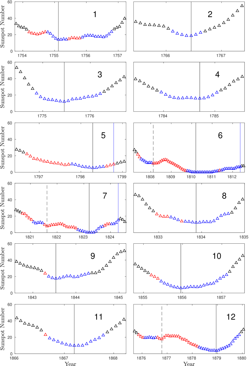
Figure 7: Triangles are monthly smoothed sunspot numbers for cycles 1$-$12, and the blue and red triangles are the potential periods of solar minimum. Red and blue indicate the trend of sunspot number is less and not less than 0. The black dashed and solid lines represent the potential solar minimum, and the blue lines indicate the position of the upper limit of $CI_{t_{e}}$.

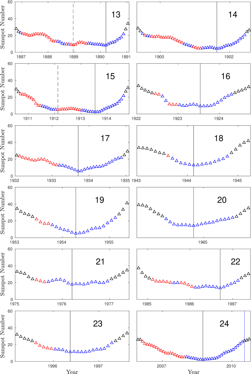
Figure 8: Same as Figure 7 but for cycles 13$-$24.

Firstly, the mean and standard deviation of the amplitudes of solar minima for cycles 1$-$23 are 9.6 and 5.6 respectively, so that the confidence interval (CI) of the amplitude of solar minimum at 99% significant level is $CI_{S}=(-5,24)$. Secondly, the mean and standard deviation of the end time of cycles 1$-$23 are 132 months and 14 months, respectively, and thus the CI of end time at 99% significant level is $CI_{t_{e}}=(95,169)$. The blue and red triangles in Figures 7 and 8 show the periods that meet the above two conditions for cycles 1$-$24, which can be called potential periods of solar minimum. The blue vertical lines in the figures indicate the position of the upper limit of $CI_{t_{e}}$.

We define that a potential solar minimum should have sunspot number less than that in the previous months and less than or equal to that in the next 8 months during the potential period of solar minimum. Based on the standards, the potential minima are obtained and presented by the black dashed and solid lines in Figures 7 and 8, where the solid lines indicate the solar minima while the dashed lines indicate the local minima but not the solar minima.

In order to determine whether a potential minimum is a solar minimum, we use the trend of sunspot number, which is defined as the slope of the linear fitting for the current month and the next 14 months monthly sunspot number. In Figures 7 and 8, the blue triangles indicate that the trend is greater than or equal to 0, and the red triangles denote that the trend is less than 0. We can find that the trends of all of the black dashed lines are less than 0 while those of black solid lines are greater than or equal to 0. Therefore, a potential minimum is determined as a solar minimum if the trend is greater than or equal to 0. This is a quasi-online method from which we can obtain the moment of solar minimum of a new cycle 14 months after the solar minimum. For Version 1 sunspot number, the method is valid for solar cycles 1-24.

5.3 Comparison of prediction ability with other functions

Since the prediction models established by Hathaway et al. (1994) and Du (2011) are based on Version 1 sunspot number, we adopt the above procedure in subsections 5.1 and 5.2 to establish a new prediction model with Version 1 sunspot number for comparison purpose. The equations corresponding to Equations (27) and (29) are given by:

$$x_{e}=0.9750x_{m}-40.13$$ (30)

and

$$x_{m}^{n}=g^{n} \equiv 1793E_{2}^{n-2}-3198E_{4}^{n-2}+2457E_{5}^{n-2}$$ (31)

$$+2472E_{4}^{n-1}+2302E_{5}^{n-1}-747T_{c}^{n-1}-12297.$$

The prediction results are exhibited in Table 6. Note that, Hathaway et al. (1994) predicted the amplitude $a$ rather than the sunspot maximum, and the predicted $a$ and starting time of a solar cycle are used to predict the rest behavior of the cycle. The comparison shows that our prediction model can obtain a good prediction result earlier than other models for predicting Version 1 sunspot number. What’s more, our prediction model can predict the cycle length simultaneously.

5.4 Prediction of solar cycle 24

Solar cycle 24 starts in December 2008 and has progressed $\sim 9$ years, which is long enough so that the parameters of the fitting function can be determined with high accuracy (e.g., Hathaway et al., 1994; Du, 2011). Thus, Equations (1), (2) and (14) can be used to estimate the sunspot number in the remaining part of the cycle by fitting the $\sim 9$ years data of cycle 24, and the estimated value can be used to compare with the prediction result by TMLP.

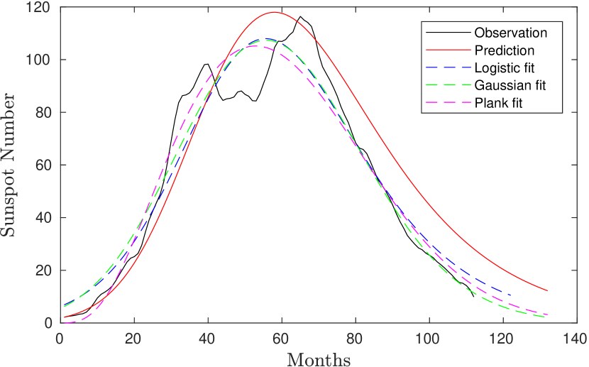
Figure 9: Monthly smoothed sunspot number curve (black line), the fitting results by the four-parameter modified logistic differential equation (blue dashed line), the four-parameter modified Gaussian function (green dashed line), the three-parameter quasi-Plank function (pink dashed line), and the TMLP predicting result (red line), for cycle 24. The cycle lengths of the red line and the blue dashed line are obtained by Equation (22) while those of the green and pink dashed line are assigned to 11 years.

The red and black curves in Figure 9 show the TMLP result and the observation for solar cycle 24, respectively. The pink, green and blue dashed curves indicate the fitting results by the quasi-Plank function Equation (1) (Hathaway et al., 1994), modified Gaussian function Equation (2) (Du, 2011) and the four-parameter modified logistic differential equation Equation (14), respectively. The cycle length from Equation (22) by fitting Equation (14) to $\sim 9$ years observed data and that of the prediction result by TMLP are 10.1 and 11.0 years, respectively. Note that, the cycle lengths of Equation (1) and Equation (2) are taken as 11 years. In order to estimate the error of prediction result, the CI of prediction result at 95% significant level should be obtained by calculating the prediction results of cycles 4$-$23. The mean and standard error of the prediction results of cycles 4$-$23 are -3.3% and 10.7%, respectively, thus the CI at 95% significant level are (-24.3%, 17.7%). Therefore, the predicted cycle length of cycle 24 by the TMLP is 11.0 (95% CI is 8.3 to 12.9) years.

The TMLP prediction result is consistent with the observation for the first 40 months of the cycle, and the sunspot number from TMLP prediction is higher than other curves after about 70 months but without larger error, i.e., the relative errors of $S_{m}$ and $T_{a}$ are 1.4% and 12%, respectively.

6 Conclusions

In this paper, we use the logistic function to study the time profile of monthly smoothed sunspot number. Due to the fact that the variations of sunspot number is asymmetrical in cycles, we introduce an asymmetry $\alpha$ to modify the logistic function. There are three parameters in addition in the function, namely, maximum cumulative sunspot number or total sunspot number $x_{m}$, initial cumulative sunspot number $x_{0}$, and maximum emergence rate $r_{0}$. By using these parameters we can give the features of solar cycles. We find that the modified logistic differential equation can fit the variations of sunspot number of solar cycles very well. The fitting results show that if we choose $\alpha=0.2$ and $r_{0}=0.224$, the four-parameter function is reduced to a two-parameter one.

Although the fitting results of the four-parameter function are slightly better than those of the two-parameter one, it is hard to establish a prediction model of sunspot number with four parameters. Therefore, we use the two-parameter modified logistic differential equation to construct the prediction model of the sunspot number in solar cycles. At the start of a cycle the parameter $x_{m}$ is estimated with a linear expression of the Shannon entropy values of the three previous cycles and the last cycle length. The correlation coefficient of the linear regression is 0.96, and the regression is significant at nearly 100% confidence level. The other parameter $x_{0}$ could be solved by taking the known quantities $S_{0}$, the sunspot number of the first month, and $x_{m}$ into Equation (24). Therefore, the sunspot number variations in a solar cycle can be predicted at the start of the cycle by the two-parameter modified logistic differential equation if the solar minimum is already known. Furthermore, we introduce a quasi-online method to determine the moment of solar minimum when 14 months after a new cycle starts. The prediction model is called TMLP in this paper, and its predicting results of solar cycles $4-23$ are all good except for cycles 5, 9, and 19. For Version 2 sunspot number, the average relative error of the solar maximum is 8.8%. The average relative errors of the ascent time is 17%, however, it would be reduced to 14% if cycle 5 is removed. In addition, the average relative error of cycle length, which is not predicted by other fitting functions in the literature, is 9.5%. In order to compare the prediction ability of TMLP with other fitting functions, we also establish a prediction model and obtain its prediction results for Version 1 sunspot number. The comparison shows that TMLP can obtain a good prediction result earlier than other fitting functions and predict the cycle length simultaneously.

Furthermore, using the TMLP, we get the prediction of the sunspot number variations of solar cycle 24, which is compared with the observation and the fitting results by the three-parameter quasi-Plank function (Hathaway et al., 1994), four-parameter modified Gaussian function (Du, 2011) and the four-parameter modified logistic differential equation. The comparison indicates that the sunspot number predicted by TMLP is consistent with the observation at the first 40 months, but is relatively larger than other curves after about 70 months. The relative errors of the solar maximum and ascent time are 1.4% and 12%, respectively. The TMLP model also predicts that the length of cycle 24 is 11.0 (95% CI is 8.3 to 12.9) years, which is slightly larger than the fitting results of the four-parameter modified logistic differential equation. The predicted cycle length of cycle 24 is similar with other works, such as 11.33 years of Uzal et al. (2012), 11.3 years of Pishkalo (2014), and 11.01 years of Kakad et al. (2017b).

We plan to predict sunspot number variations of solar cycle 25 when we can determine the solar minimum, i.e., 14 months after the solar minimum of the cycle.

Table 1: Fitted parameters of the four-parameter modified logistic differential equation, the variances and covariances of these parameters, the evaluating indices, and the absolute relative error of cycle features for cycles $1-23$.

Cycle No.	$\alpha$	$r_{0}$	$x_{0}$	$x_{m}$	$\sigma^{2}_{\alpha\alpha}$	$\sigma^{2}_{r_{0}r_{0}}$	$\sigma^{2}_{x_{0}x_{0}}$	$\sigma^{2}_{x_{m}x_{m}}$	$\sigma^{2}_{\alpha r_{0}}$	$\sigma^{2}_{\alpha x_{0}}$	$\sigma^{2}_{\alpha x_{m}}$	$\sigma^{2}_{r_{0}x_{0}}$	$\sigma^{2}_{r_{0}x_{m}}$	$\sigma^{2}_{x_{0}x_{m}}$	$x_{e}$	$A^{2}$	$\sigma$	$CC$	$\frac{\delta S_{m}}{S_{m}}$	$\frac{\delta T_{a}}{T_{a}}$
1	9.12 $\pm$ 1.17 E-1	5.06 $\pm$ 0.46 E-2	2.74 $\pm$ 0.48 E+2	1.03 $\pm$ 0.01 E+4	1.4 E-2	2.1 E-5	2.3 E+3	1.7 E+4	-5.3 E-4	5.2 E+0	3.5 E-1	-2.1 E-1	-8.6 E-2	2.0 E+3	9.74 E+3	71	8.5	0.973	15%	4.1%
2	2.64 $\pm$ 0.61 E-1	1.79 $\pm$ 0.37 E-1	1.49 $\pm$ 0.34 E+2	1.15 $\pm$ 0.01 E+4	3.8 E-3	1.3 E-3	1.2 E+3	1.7 E+4	-2.2 E-3	1.9 E+0	-2.1 E-1	-1.2 E+0	-8.7 E-2	9.8 E+2	1.09 E+4	66	9.8	0.983	8.9%	11%
3	3.49 $\pm$ 0.64 E-2	1.57 $\pm$ 0.28 E+0	5.65 $\pm$ 1.35 E+0	1.24 $\pm$ 0.01 E+4	4.0 E-5	7.8 E-2	1.8 E+0	2.1 E+4	-1.8 E-3	3.9 E-3	-1.7 E-2	-2.0 E-1	-1.3 E+0	1.0 E+2	1.22 E+4	16	13	0.987	7.1%	12%
4	2.74 $\pm$ 0.41 E-2	1.31 $\pm$ 0.19 E+0	1.34 $\pm$ 0.15 E+2	1.69 $\pm$ 0.01 E+4	1.7 E-5	3.7 E-2	2.2 E+2	3.7 E+4	-7.9 E-4	1.3 E-2	-1.5 E-2	-8.3 E-1	-1.6 E+0	1.7 E+3	1.67 E+4	58	14	0.982	6.3%	11%
5	8.78 $\pm$ 1.38 E-1	6.11 $\pm$ 0.70 E-2	1.16 $\pm$ 0.29 E+2	6.00 $\pm$ 0.08 E+3	1.9 E-2	4.9 E-5	8.2 E+2	7.7 E+3	-9.5 E-4	3.7 E+0	1.9 E+0	-2.0 E-1	-1.5 E-1	9.3 E+2	5.90 E+3	25	6.6	0.973	2.0%	24%
6	4.30 $\pm$ 0.66 E-1	1.19 $\pm$ 0.15 E-1	2.40 $\pm$ 1.39 E+0	4.74 $\pm$ 0.06 E+3	4.4 E-3	2.4 E-4	1.9 E+0	4.3 E+3	-1.0 E-3	8.7 E-2	2.5 E-1	-2.1 E-2	-1.4 E-1	2.3 E+1	4.65 E+3	8.9	5.1	0.979	8.9%	6.3%
7	1.28 $\pm$ 0.14 E+0	4.84 $\pm$ 0.33 E-2	1.79 $\pm$ 0.31 E+2	8.53 $\pm$ 0.10 E+3	1.8 E-2	1.1 E-5	9.3 E+2	1.0 E+4	-4.4 E-4	3.8 E+0	9.9 E-1	-9.9 E-2	-6.8 E-2	1.0 E+3	8.21 E+3	54	7.4	0.982	2.0%	5.2%
8	4.07 $\pm$ 0.84 E-2	1.15 $\pm$ 0.23 E+0	2.30 $\pm$ 0.41 E+1	1.34 $\pm$ 0.01 E+4	7.1 E-5	5.4 E-2	1.7 E+1	2.2 E+4	-2.0 E-3	1.7 E-2	-4.6 E-2	-5.3 E-1	-2.2 E-1	3.1 E+2	1.29 E+4	25	12	0.985	7.9%	4.7%
9	2.24 $\pm$ 0.58 E-1	1.68 $\pm$ 0.39 E-1	6.49 $\pm$ 2.40 E+1	1.54 $\pm$ 0.02 E+4	3.3 E-3	1.5 E-3	5.8 E+2	4.5 E+4	-2.2 E-3	1.3 E+0	-5.1 E-1	-8.9 E-1	-6.5 E-2	1.1 E+3	1.48 E+4	63	15	0.971	13%	13%
10	3.14 $\pm$ 0.63 E-2	1.20 $\pm$ 0.24 E+0	1.57 $\pm$ 0.30 E+1	1.29 $\pm$ 0.01 E+4	4.0 E-5	5.6 E-2	9.0 E+0	2.3 E+4	-1.5 E-3	7.2 E-3	-4.7 E-2	-3.1 E-1	3.5 E-2	2.5 E+2	1.24 E+4	44	11	0.980	5.0%	5.6%
11	1.60 $\pm$ 0.39 E-1	3.12 $\pm$ 0.71 E-1	3.82 $\pm$ 1.17 E+1	1.27 $\pm$ 0.01 E+4	1.5 E-3	5.0 E-3	1.4 E+2	1.5 E+4	-2.8 E-3	4.3 E-1	-1.1 E-1	-7.9 E-1	-8.9 E-2	2.9 E+2	1.25 E+4	6.7	10	0.990	8.2%	8.7%
12	7.19 $\pm$ 1.56 E-1	7.29 $\pm$ 1.21 E-2	2.43 $\pm$ 0.63 E+2	8.13 $\pm$ 0.13 E+3	2.4 E-2	1.4 E-4	3.9 E+3	1.7 E+4	-1.9 E-3	9.2 E+0	3.7 E+0	-7.3 E-1	-3.9 E-1	3.2 E+3	8.03 E+3	43	9.7	0.970	6.1%	13%
13	4.08 $\pm$ 0.46 E-2	1.03 $\pm$ 0.11 E+0	5.28 $\pm$ 0.37 E+1	9.38 $\pm$ 0.05 E+3	2.1 E-5	1.3 E-2	1.4 E+1	3.2 E+3	-5.1 E-4	7.0 E-3	-6.4 E-3	-2.0 E-1	-1.0 E-1	1.1 E+2	9.24 E+3	11	4.4	0.995	3.0%	9.3%
14	3.66 $\pm$ 0.97 E-1	1.20 $\pm$ 0.27 E-1	1.06 $\pm$ 0.34 E+2	7.91 $\pm$ 0.11 E+3	9.1 E-3	7.2 E-4	1.1 E+3	1.2 E+4	-2.6 E-3	3.0 E+0	1.0 E+0	-8.7 E-1	-4.2 E-1	1.1 E+3	7.72 E+3	49	8.6	0.973	1.3%	9.1%
15	4.86 $\pm$ 0.80 E-1	1.16 $\pm$ 0.15 E-1	8.27 $\pm$ 2.22 E+1	9.16 $\pm$ 0.12 E+3	6.3 E-3	2.3 E-4	4.9 E+2	1.6 E+4	-1.2 E-3	1.6 E+0	-4.2 E-1	-3.3 E-1	-7.2 E-2	5.9 E+2	8.97 E+3	18	10	0.980	13%	5.7%
16	4.02 $\pm$ 0.85 E-1	1.21 $\pm$ 0.22 E-1	1.22 $\pm$ 0.32 E+2	8.74 $\pm$ 0.10 E+3	7.2 E-3	4.6 E-4	1.0 E+3	1.1 E+4	-1.8 E-3	2.6 E+0	4.4 E-1	-6.6 E-1	-2.2 E-1	8.2 E+2	8.48 E+3	38	8.1	0.982	0.39%	14%
17	5.24 $\pm$ 0.77 E-2	8.06 $\pm$ 1.15 E-1	9.29 $\pm$ 1.41 E+0	1.25 $\pm$ 0.00 E+4	5.9 E-5	1.3 E-2	2.0 E+0	7.3 E+3	-8.9 E-4	7.5 E-3	-3.8 E-2	-1.2 E-1	2.0 E-1	4.8 E+1	1.20 E+4	57	6.6	0.994	4.4%	15%
18	1.25 $\pm$ 0.34 E-1	3.63 $\pm$ 0.91 E-1	4.00 $\pm$ 1.12 E+1	1.39 $\pm$ 0.01 E+4	1.1 E-3	8.3 E-3	1.2 E+2	1.5 E+4	-3.0 E-3	3.5 E-1	-2.2 E-1	-9.6 E-1	3.1 E-1	2.2 E+2	1.34 E+4	58	9.7	0.991	0.020%	17%
19	6.94 $\pm$ 0.86 E-2	6.97 $\pm$ 0.83 E-1	1.95 $\pm$ 0.24 E+1	1.66 $\pm$ 0.00 E+4	7.4 E-5	6.9 E-3	5.6 E+0	7.3 E+3	-7.1 E-4	1.6 E-2	-4.1 E-2	-1.6 E-1	1.8 E-1	6.2 E+1	1.63 E+4	18	7.3	0.997	0.45%	6.7%
20	4.44 $\pm$ 0.82 E-2	7.87 $\pm$ 1.43 E-1	5.91 $\pm$ 0.63 E+1	1.26 $\pm$ 0.01 E+4	6.8 E-5	2.0 E-2	4.0 E+1	1.1 E+4	-1.2 E-3	2.7 E-2	-4.3 E-2	-5.1 E-1	2.2 E-1	3.2 E+2	1.20 E+4	65	7.3	0.989	1.0%	5.7%
21	2.29 $\pm$ 0.43 E-1	2.11 $\pm$ 0.35 E-1	5.31 $\pm$ 1.48 E+1	1.46 $\pm$ 0.01 E+4	1.8 E-3	1.2 E-3	2.2 E+2	1.5 E+4	-1.5 E-3	5.9 E-1	-4.5 E-2	-5.0 E-1	-1.2 E-1	3.2 E+2	1.42 E+4	48	10	0.992	0.22%	9.8%
22	1.20 $\pm$ 0.41 E-1	4.06 $\pm$ 1.30 E-1	4.88 $\pm$ 1.51 E+1	1.31 $\pm$ 0.01 E+4	1.6 E-3	1.7 E-2	2.3 E+2	1.9 E+4	-5.3 E-3	5.7 E-1	-2.5 E-1	-1.8 E+0	3.7 E-1	3.8 E+2	1.28 E+4	42	12	0.987	4.1%	11%
23	3.63 $\pm$ 0.47 E-1	1.27 $\pm$ 0.14 E-1	1.03 $\pm$ 0.20 E+2	1.26 $\pm$ 0.01 E+4	2.2 E-3	2.0 E-4	3.9 E+2	1.0 E+4	-6.6 E-4	8.7 E-1	7.5 E-2	-2.7 E-1	-9.7 E-2	4.5 E+2	1.24 E+4	20	7.9	0.992	0.70%	18%
avg.	3.17 E-1	4.79 E-1														39	9.3	0.984	5.2%	10%
s.d.	3.39 E-1	4.80 E-1														21	2.6	0.008	4.5%	4.9%

Table 2: Same as Table 1 but for the two-parameter function.

Cycle No.	$x_{0}$	$x_{m}$	$\sigma_{x_{0}x_{0}}$	$\sigma_{x_{m}x_{m}}$	$\sigma_{x_{0}x_{m}}$	$x_{e}$	$A^{2}$	$\sigma$	$CC$	$\frac{\delta S_{m}}{S_{m}}$	$\frac{\delta T_{a}}{T_{a}}$
1	2.50 $\pm$ 0.37 E+0	8.88 $\pm$ 0.16 E+3	1.2 E-1	2.3 E+4	6.1 E+0	8.47 E+3	191	17	0.890	7.6%	12%
2	1.33 $\pm$ 0.06 E+2	1.16 $\pm$ 0.01 E+4	3.1 E+1	1.0 E+4	1.1 E+2	1.09 E+4	93	10	0.982	9.9%	11%
3	2.05 $\pm$ 0.17 E+2	1.41 $\pm$ 0.02 E+4	2.6 E+2	6.8 E+4	9.8 E+2	1.35 E+4	219	27	0.941	20%	16%
4	1.40 $\pm$ 0.09 E+2	1.57 $\pm$ 0.01 E+4	6.8 E+1	3.2 E+4	2.9 E+2	1.56 E+4	347	20	0.961	0.027%	11%
5	4.64 $\pm$ 0.43 E+0	5.73 $\pm$ 0.07 E+3	1.8 E-1	6.2 E+3	4.9 E+0	5.58 E+3	46	7.9	0.961	4.8%	32%
6	1.86 $\pm$ 0.15 E-1	4.83 $\pm$ 0.05 E+3	2.2 E-4	2.9 E+3	1.1 E-1	4.68 E+3	36	5.4	0.977	11%	5.1%
7	1.66 $\pm$ 0.17 E+0	8.20 $\pm$ 0.11 E+3	2.9 E-2	1.3 E+4	2.3 E+0	7.63 E+3	185	12	0.957	3.2%	16%
8	1.62 $\pm$ 0.09 E+2	1.41 $\pm$ 0.01 E+4	8.2 E+1	3.0 E+4	3.4 E+2	1.36 E+4	98	18	0.970	13%	8.9%
9	1.06 $\pm$ 0.10 E+1	1.39 $\pm$ 0.01 E+4	8.3 E-1	3.2 E+4	2.4 E+1	1.37 E+4	84	19	0.949	4.9%	11%
10	3.48 $\pm$ 0.23 E+1	1.23 $\pm$ 0.01 E+4	5.1 E+0	1.9 E+4	5.4 E+1	1.20 E+4	46	14	0.967	0.68%	7.3%
11	1.18 $\pm$ 0.06 E+2	1.34 $\pm$ 0.01 E+4	3.1 E+1	1.7 E+4	1.5 E+2	1.32 E+4	63	14	0.982	14%	11%
12	4.55 $\pm$ 0.34 E+1	7.89 $\pm$ 0.10 E+3	1.2 E+1	1.1 E+4	6.4 E+1	7.73 E+3	27	11	0.964	4.8%	22%
13	1.26 $\pm$ 0.04 E+2	9.43 $\pm$ 0.05 E+3	1.4 E+1	3.4 E+3	4.7 E+1	9.32 E+3	30	5.9	0.992	3.4%	6.8%
14	2.88 $\pm$ 0.21 E+1	7.53 $\pm$ 0.09 E+3	4.6 E+0	9.1 E+3	3.5 E+1	7.38 E+3	30	9.6	0.966	5.5%	5.7%
15	4.80 $\pm$ 0.31 E+1	9.66 $\pm$ 0.12 E+3	9.3 E+0	1.4 E+4	6.7 E+1	9.24 E+3	89	12	0.971	18%	2.0%
16	5.44 $\pm$ 0.28 E+1	8.71 $\pm$ 0.08 E+3	7.6 E+0	6.9 E+3	4.2 E+1	8.39 E+3	49	8.3	0.981	0.36%	16%
17	4.36 $\pm$ 0.15 E+1	1.26 $\pm$ 0.00 E+4	2.2 E+0	6.3 E+3	2.1 E+1	1.21 E+4	45	7.9	0.992	4.8%	19%
18	9.36 $\pm$ 0.36 E+1	1.42 $\pm$ 0.01 E+4	1.2 E+1	1.1 E+4	7.0 E+1	1.37 E+4	86	11	0.989	2.3%	18%
19	1.57 $\pm$ 0.07 E+2	1.78 $\pm$ 0.01 E+4	4.4 E+1	2.5 E+4	2.2 E+2	1.73 E+4	129	17	0.984	6.4%	2.1%
20	4.43 $\pm$ 0.32 E+1	1.14 $\pm$ 0.01 E+4	8.3 E+0	1.6 E+4	6.0 E+1	1.12 E+4	44	14	0.959	9.6%	5.7%
21	7.10 $\pm$ 0.29 E+1	1.51 $\pm$ 0.01 E+4	7.5 E+0	1.2 E+4	5.6 E+1	1.46 E+4	106	12	0.989	3.0%	9.8%
22	1.67 $\pm$ 0.09 E+2	1.39 $\pm$ 0.01 E+4	6.6 E+1	2.1 E+4	2.6 E+2	1.34 E+4	135	15	0.977	1.9%	13%
23	3.26 $\pm$ 0.14 E+1	1.23 $\pm$ 0.00 E+4	1.9 E+0	7.8 E+3	2.1 E+1	1.22 E+4	15	8.9	0.990	2.6%	22%
avg.							95	13	0.969	6.6%	12%
s.d.							78	5.2	0.022	5.5%	7.1%

Table 3: Comparison of fitting effects between the modified logistic differential equation with modified Gaussian function and quasi-Plank function.

Sunspot	Function	Number of	$\overline{A^{2}}$	$\overline{\sigma}$	$\overline{r}$	$\overline{BIC}$	$\overline{\delta R_{m}/R_{m}}$	$\overline{\delta T_{a}/T_{a}}$
Version		Parameters
V1	L	4	24	5.8	0.984	851	5.3%	10%
	L	3	39	6.4	0.980	874	5.5%	12%
	L	2	59	8.0	0.969	917	6.8%	12%
	G	4	53	5.2	0.986	823	5.2%	9.4%
	P	3	25	6.8	0.978	885	7.7%	13%
V2	L	4	39	9.3	0.984	981	5.2%	10%
	L	3	64	10	0.980	1004	5.3%	12%
	L	2	95	13	0.969	1048	6.6%	12%
	G	4	89	8.4	0.986	953	5.1%	9.5%
	P	3	42	11	0.978	1014	7.6%	13%

Table 4: Shannon entropy of each phase, which are calculated by the monthly sunspot number, and cycle length for solar cycles $1-23$.

Cycle No.	$E_{1}$	$E_{2}$	$E_{3}$	$E_{4}$	$E_{5}$	$T_{c}$
1	5.0	5.9	5.9	6.4	5.2	11.3
2	5.6	6.7	7.6	6.8	6.0	9.0
3	5.8	7.4	6.5	6.7	4.7	9.3
4	6.3	6.6	5.8	6.0	5.3	13.6
5	5.1	5.3	5.5	4.8	4.4	11.9
6	4.0	5.2	6.6	6.0	5.1	13.0
7	5.4	6.0	6.1	6.9	5.6	10.7
8	6.3	7.4	6.9	6.9	5.7	9.7
9	5.6	7.2	6.9	6.4	5.4	12.4
10	4.9	6.5	6.5	6.2	5.6	11.3
11	6.2	7.2	6.4	6.0	4.7	11.8
12	5.6	6.5	6.3	5.7	4.6	11.3
13	5.9	6.6	6.1	6.1	4.5	11.8
14	5.7	6.6	7.2	6.3	4.4	11.5
15	5.4	6.3	7.2	6.2	5.3	10.0
16	5.5	6.4	6.2	6.5	4.7	10.2
17	5.1	6.7	7.1	6.7	6.2	10.4
18	5.8	6.7	7.2	6.2	5.7	10.2
19	5.6	7.0	6.7	6.0	5.4	10.5
20	5.2	6.5	5.5	5.9	5.3	11.4
21	5.7	6.9	7.0	6.5	5.1	10.5
22	5.8	6.7	6.7	6.2	5.2	9.7
23	5.6	6.7	6.6	5.8	4.7	12.6

Table 5: Predicted parameters from TMLP model, the evaluating indices, and the absolute relative error of cycle features for cycles $4-23$.

Cycle No.	$x_{0}$	$x_{m}$	$A^{2}$	$\sigma$	$CC$	$\frac{\delta S_{m}}{S_{m}}$	$\frac{\delta T_{a}}{T_{a}}$	$\frac{\delta T_{c}}{T_{c}}$
4	1.13 E+2	1.60 E+4	2.2 E+2	21	0.957	2.0%	15%	22%
5	3.75 E+1	5.53 E+3	4.5 E+2	18	0.768	1.1%	71%	16%
6	1.09 E+0	5.97 E+3	1.2 E+2	14	0.821	10%	5.7%	8.8%
7	1.08 E+0	7.63 E+3	3.1 E+2	13	0.944	3.9%	13%	14%
8	8.41 E+1	1.54 E+4	3.4 E+2	30	0.909	5.5%	18%	11%
9	1.29 E+2	1.42 E+4	2.1 E+3	50	0.574	2.9%	20%	16%
10	3.88 E+1	1.38 E+4	4.5 E+1	19	0.940	11%	7.4%	1.9%
11	6.72 E+1	1.43 E+4	2.5 E+2	22	0.954	8.4%	18%	8.3%
12	2.40 E+1	8.21 E+3	1.7 E+2	14	0.938	1.0%	11%	4.6%
13	5.88 E+1	8.48 E+3	7.3 E+1	14	0.952	13%	4.2%	13%
14	3.02 E+1	7.10 E+3	2.7 E+1	10	0.961	0.50%	3.9%	9.3%
15	1.55 E+1	9.15 E+3	5.4 E+2	22	0.906	22%	14%	11%
16	6.62 E+1	1.01 E+4	4.5 E+1	15	0.937	16%	19%	2.3%
17	3.80 E+1	1.17 E+4	4.8 E+1	12	0.982	12%	19%	4.4%
18	9.12 E+1	1.34 E+4	8.3 E+1	13	0.983	8.1%	19%	3.5%
19	3.21 E+1	1.54 E+4	1.3 E+3	50	0.849	19%	16%	7.1%
20	1.04 E+2	1.20 E+4	3.7 E+2	21	0.906	15%	6.5%	9.5%
21	1.31 E+2	1.39 E+4	2.1 E+2	24	0.953	10%	2.2%	1.4%
22	9.60 E+1	1.34 E+4	3.3 E+2	21	0.956	5.1%	21%	8.6%
23	7.80 E+1	1.31 E+4	2.0 E+2	19	0.953	9.3%	35%	16%
avg.			3.6 E+2	21	0.907	8.8%	17%	9.5%
s.d.			4.9 E+2	11	0.095	6.2%	15%	5.6%

Table 6: Comparison of prediction results between TMLP with modified Gaussian function and quasi-Plank function.

Function	$\Delta t$ (month)	$\delta R_{m}/R_{m}$	$\delta a/a$	$\delta T_{c}/T_{c}$
L	15	12%	—	9.2%
G	25	15%	—	—
P	30	—	20%	—
P	42	—	10%	—

References

- Balakrishnan (2010) Balakrishnan, N. 2010, Handbook of the logistic distribution, 2nd Edition (Boca Raton, CRC Press)
- Bevington & Robinson (2003) Bevington, P. R., & Robinson, D. K. 2003, Data Reduction and Error Analysis for the Physical Sciences, ed. P. R. Bevington & K. D. Robinson (3rd ed.; Boston, MA: McGraw-Hill)
- Birch (1999) Birch, C. 1999, Annals of Botany, 83, 713
- Clette et al. (2015) Clette, F., Cliver, E. W., Lefèvre, L., Svalgaard, L., & Vaquero, J. M. 2015, SpWea, 13, 529
- Du (2011) Du, Z. 2011, Sol. Phys., 273, 231
- Fletcher (1987) Fletcher, R. 1987, Practical methods of optimization, 2nd Edition (New York, Wiley)
- Gnevyshev (1963) Gnevyshev, M. N. 1963, SvA, 7, 311
- Haigh (2007) Haigh, J. D. 2007, LRSP, 4
- Hathaway (2015) Hathaway, D. H. 2015, LRSP, 12
- Hathaway et al. (1994) Hathaway, D. H., Wilson, R. M., & Reichmann, E. J. 1994, Sol. Phys., 151, 177
- Holland & Vaughan (1984) Holland, R. L., & Vaughan, W. W. 1984, J. Geophys. Res., 89, 11
- Kakad (2011) Kakad, B. 2011, Sol. Phys., 270, 393
- Kakad et al. (2015) Kakad, B., Kakad, A., & Ramesh, D. S. 2015, JSWSC, 5, A29
- Kakad et al. (2017a) Kakad, B., Kakad, A., & Ramesh, D. S. 2017a, Sol. Phys., 292, 1
- Kakad et al. (2017b) Kakad, B., Kakad, A., & Ramesh, D. S. 2017b, Sol. Phys., 292, 181,
- Laurenza et al. (2012) Laurenza, M., Consolini, G., Storini, M., & Damiani, A. 2012, ASTRA, 8, 19
- Li et al. (2017) Li, F. Y., Xiang, N. B., Kong, D. F., & Xie, J. L. 2017, ApJ, 834, 192
- Li (1999) Li, K. 1999, A&A, 345, 1006
- McDonald (1998) McDonald, F. B. 1998, Space Sci. Rev., 83, 33
- Pishkalo (2014) Pishkalo, M. I. 2014, Sol. Phys., 289, 1815
- Qin & Shen (2017) Qin, G., & Shen, Z.-N. 2017, ApJ, 846, 56
- Qin & Zhao (2013) Qin, G., & Zhao, L.-L. 2013, arxiv:1312.2296
- Richards (1959) Richards, F. J. 1959, Journal of Experimental Botany, 10, 290
- Roshchina & Sarychev (2011) Roshchina, E. M., & Sarychev, A. P. 2011, SoSyR, 45, 539
- Sabarinath & Anilkumar (2008) Sabarinath, A., & Anilkumar, A. K. 2008, Sol. Phys., 250, 183
- Schwarz (1978) Schwarz, Gideon E. 1978, Annals of Statistics, 6, 461
- Shannon (1948) Shannon, C. E. 1948, Bell Syst. Tech. J., 27, 379
- Shen & Qin (2018) Shen, Z.-N., & Qin, G. 2018, ApJ, 854, 137
- Stewart & Panofsky (1938) Stewart, J. Q., & Panofsky, H. A. A. 1938, ApJ, 88, 385
- Uzal et al. (2012) Uzal, L. C., Piacentini, R. D., & Verdes, P. F. 2012, Sol. Phys., 279, 551
- Verhulst (1838) Verhulst, P. F. 1838, Correspondance Mathématique et Physique, 10, 113
- Volobuev (2009) Volobuev, D. M. 2009, Sol. Phys., 258, 319
- Wu & Qin (2018) Wu, S.-S., & Qin, G. 2018, JGRA, 123, 76