Motion of a superconducting loop in an inhomogeneous magnetic field:
a didactic experiment
Abstract
We present an experiment conductive to an understanding of both Faraday’s law and the properties of the superconducting state. It consists in the analysis of the motion of a superconducting loop moving under the influence of gravity in an inhomogeneous horizontal magnetic field. Gravity, conservation of magnetic flux, and friction combine to give damped harmonic oscillations. The measured frequency of oscillation and the damping constant as a function of the magnetic field strength (the only free parameter) are in good agreement with the theoretical model.
pacs:
01.50.Pa, 01.40.GmI Introduction
High temperature superconductors have not only brought new applications and an increase of the general interest in superconductivity, but also the possibility to introduce with relative ease university students to actual experiments.
A number of didactic experiments have been described in the literature esperimenti and laboratory kits are available for many of them kits .
The following experiment can help students get acquainted with superconductivity by describing and visualizing in a fascinating way one of the most well known aspects of superconductivity: magnetic levitation induced by super-currents. While conceptually simple, the complexity of the apparatus –even in its simpler high temperature version– makes it suitable for a graduate lab; to make it more accessible, video recordings can be made that could be used for in class presentations.
Due to Faraday’s law, a time dependent magnetic field induces currents in a conducting circuit. The same result is obtained when the circuit moves in an inhomogeneous magnetic field. In the case of an ohmic conductor, these currents are heavily damped by the circuit resistance , as the damping time constant L/R – being the circuit inductance– is usually very small. However in the case of a superconducting loop the situation is different. In fact in this case –as the resistance is vanishingly small– the induced currents are persistent and the magnetic flux through the loop is therefore constant.
Allowing a conducting loop to fall under the influence of gravity in a decreasing inhomogeneous magnetic field, the induced current causes a force on the loop opposing its downwards acceleration. In the case the loop is superconducting, the only damping is mechanical and for suitably chosen parameters such that the magnetic force is strong enough to reverse the acceleration of the loop, the loop itself hangs unsupported while oscillating around its equilibrium point for sufficiently long times to allow detection of the oscillations. Note that this is a very different kind of “levitation” from the one seen in the didactic levitation experiments usually found in the literature esperimenti , which is due to the Meissner effect meissner (expulsion of the magnetic field from the superconductor).
II Theoretical model
In our experiment the loop moved in liquid helium (LHe) and not in vacuum, as discussed by Romer rom , and thus his model must be modified to take into account the dissipation due to the viscosity of the medium and the friction between the loop and parts of the apparatus. Using a high temperature conductor permits to avoid the use of LHe; in the following sections we shall indicate in italics changes in the apparatus and procedure for this simpler experiment.
Let’s consider a rectangular loop of height and width that moves in a given medium under the influence of gravity (directed downward) in a magnetic field (directed out of the page) as in Figure 1.
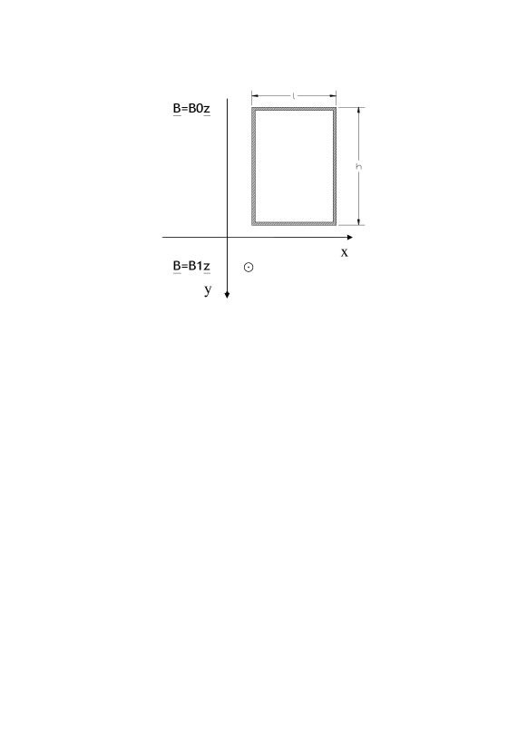
Let’s moreover assume that:
1. the magnetic field is horizontal, uniform and of constant magnitude for and for (note that the axis is pointing downward);
2. The loop is kept vertical and its motion is along the vertical axis so that the magnetic force is also vertical and the problem can be considered to be one dimensional;
3. for simplicity, all damping effects, even those due to friction with the apparatus, are described as a single viscous force linear in the loop vertical velocity where the dot denotes, as usual, differentiation with respect to time.
Suppose the loop is released from rest with its lower edge in with no initial current. As it falls down, it progressively leaves the region with magnetic field and enters the zone with field and a current begins to circulate, in order to maintain constant the initial magnetic flux. When the lower edge of the loop is in , the concatenated outward flux of is given by:
| (1) |
where is the current (taken positive if flowing counterclockwise) and is the self-inductance of the loop. Therefore, denoting by the mass and by the resistance of the loop, from Faraday’s law we have:
| (2) |
Note that when the loop leaves the region , the current does not depend on any longer but becomes constant: for and for . Care must therefore be taken to design the experiment to avoid these discontinuities and keep the motion of the loop within and . We now write Newton’s law of motion for the loop, subjected to the three forces gravitational, magnetic, and viscous:
| (3) |
where is the usual gravitational acceleration on the earth surface. Differentiating equation (2) and using equations (2) and (3) to eliminate , we obtain for the well known equation of damped harmonic oscillations:
| (4) |
with:
The equation for is in general more complicated than above, depending on a time-dependent driving force. Luckily superconductivity simplifies things: when , equation 2 reduces to the proportionality relation . Since we have chosen both initial conditions and to be zero, the same proportionality relation holds between and , and the resulting equation of motion is again the equation for damped harmonic motion:
| (5) |
the only difference with eq. 4 being in the driving term that is now just itself. If we now suppose that the damping is less than critical, i.e. if , equation 5 has the following solution:
| (6) |
where
| (7) | |||
| (8) |
If this is this case, as stated in the introduction, the loop performs oscillations with a frequency and damping time constant which is almost entirely due to mechanical friction (some tiny electrical dissipation is present when using a type II superconductor, such as Niobium).
Note that the initial amplitude of the oscillations is
| (9) |
which means that to keep the loop in the region of validity of eq. 6, we need
| (10) |
III Experimental set up
The experiment has been performed with a superconducting loop cut out of a niobium (Nb) sheet weakly alloyed with 1% titanium, immersed in a LHe bath at , well below the Nb critical temperature (about ). In order to minimize the cryogenic losses of LHe, we used a cryostat where the helium vessel was surrounded by a vessel filed with liquid nitrogen (LN); both vessels were moreover double wall ones, with a vacuum chamber as insulation. A schematic view is shown in Figure 2.
A HTS (High Temperature Superconductor) material could be used for the superconducting loop. The most suitable candidate is the YBCO (Yttrium based copper oxide) coated conductor, since it is produced in thin sheets so it is relatively easier to obtain a small loop without resistive joints. YBCO has a critical temperature of , therefore the experiment could be done directly in liquid nitrogen, highly simplifying the cryostat and also reducing the cost of the experiment. Using an YBCO loop may enable even to design the experiment without cryogenic fluid: the loop could be placed in an inner chamber without cryogen and cooled by the LN surrounding the chamber via radiation and conduction (the loop could be in a N or He atmosphere). As a further advantage, in this configuration the friction would be greatly reduced (no liquid in the experiment chamber, only gas). The cooling of the chamber via a cryocooler, beside eliminating the need of cryogenic fluid, greatly reduce the complexity and operational risk. Use of a cryocooler would facilitate the carrying out of the experiment at variable temperature. In this case it would also be easy to show what happens when the temperature is slowly increased above the critical temperature.
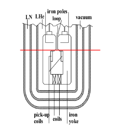
In the inner zone of the cryostat we placed an electromagnet, which generated the needed magnetic field. The poles of the magnet were apart and the cross-section of the gap was . To measure the magnetic field in operation condition, a cryogenic Hall probe was placed in a sample holder that could be moved –acting from outside the cryostat– along the axis of the magnet to map the field itself. The superconducting loop, cut from a Nb sheet, had the following dimensions: , . Its mass was and its self-inductance was ; the minimum value of required to keep the loop in the operation region is therefore about . Two guides kept the loop away from the edges of the magnet poles and limited unwanted lateral movements. They were made of G10 fiberglass and, to reduce friction, they were covered with Molykote (bi-solphure of molybdenus with some graphite powder).
To reduce the boiling of LHe in the zone of the moving loop (that could disturb the oscillations and their visibility), the two coils of the magnet have been wound using very low resistivity wires so as to give the minimum heat production once the magnetic field, suitable to keep frequency of oscillations in a “reasonable” range, has been turned on. For , the calculated evaporation, due to the heat production of the coils, was about .
Care has also been taken of always being below the critical magnetic field (which for Nb is about with a density of current of ). The “reasonable” frequency of oscillation has been chosen to be about , so that the motion could be video-recorded, both for didactic purposes (e.g. in–class presentations) and as a set up and measuring tool, as we shall explain in the following. For this purpose, a common video recorder was used.
The cryostat was designed with a double optical window, through the LN vessel and the LHe chamber, to allow a direct observation of the oscillating loop in the magnet gap between poles. The video camera could be placed in front of it, as a visual aid when setting up the experiment and to record the oscillations of the loop.
The motion of the loop was detected measuring the voltage induced in two pick-up coils by the magnetic flux that was generated by the supercurrents in the moving loop. These coils consisted of windings of diameter copper wire surrounding an area of , for a total thickness of . They were placed just below the magnet poles, where the motion of the loop took place. The voltage in the coils was registered by an oscilloscope (National VP-5730A ID4N0073B12). As the current in the pick-up coils was neglible, so were the heating around them and the braking effect due to the magnetic field they generated.
IV Experimental procedure
The experiment can be divided into four time–ordered steps.
1. The loop was placed inside the magnet gap and kept in position by a thin nylon thread fastened to the top of the cryostat.
2. The electromagnet was switched on at a given magnetic field.
3. Vacuum was made in the vacuum chamber; the external section of the cryostat was then filled with liquid nitrogen; finally, LHe was poured into the inner zone so that the transition of the loop to the superconducting state could take place.
Let us notice that steps and had to precede step because we had to place the loop in position, and in the desired magnetic field, while it was still warm. The reason why the loop had to become superconducting when the magnetic field was already linked to the loop itself is that inserting an already superconducting loop in a field region would have induced a super-current tending to expel the loop itself.
4. The thread, used to hang the loop in the proper position, was suddenly disconnected from the top of the cryostat, so that the loop was let free to fall down. As predicted the loop started to oscillate before stopping at the equilibrium position.
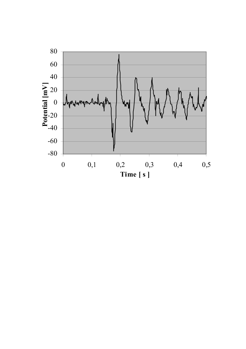
The use of the video camera was fundamental since it helped to control the filling of the cryostat and the positioning of the loop during the setup, and to afterwards check the motion of the loop itself during the experiment. Moreover, looking at the motion frame after frame, we could also get some rough measurements of the frequencies of oscillation of the loop. Of course, more refined measurements were made by means of the pick-up coils, connected to the digital oscilloscope, as described in Section III. The plots generated by the oscilloscope (see Figure 3) showed the typical behavior of damped harmonic motions: the time between two maxima was the period of the oscillation while the damping constant could be evaluated from the decreasing amplitude of the peaks.
Unfortunately the video camera and the pick-up coils could not be used at the same time, since the light source, essential to illuminate the inner cryostat, caused too much noise in the signal coming from the pick-up coils. Therefore, for each value of the magnetic field, the experiment had to be divided into two parts: the first one used the video camera for a first analysis of the motion; the second one, without the camera but with the pick-up coils switched on, measured the frequencies from the pick-up coils signal.
V Data analysis and results
We now discuss the results of the experiment, comparing the measured oscillation frequencies with the ones predicted by our model. To determine these latter values, the quantity is crucial. For our purposes the magnetic field could be considered uniform inside the magnet: for a typical operating value , is uniform up to all through the magnet gap.
The situation was different outside the magnet poles, where the magnetic field varied with the position up to . Since our model assumes a magnetic field of uniform strength outside the region between the magnet poles, a suitable average had to be considered. Our choice was to perform a spatial average limited to the region accessed by the loop. The vertical range of motion outside the magnet gap has been visually assessed with the help of the video camera to be . For this and similar measurements, a graduated scale, calibrated to match a scale placed in the cryostat before filling it and then removed, was attached to the camera monitor.
The oscillation frequencieswere measured for values of , varying from to . For each value of the field, to tests were conducted. Measurements taken in the range were dropped for two reasons; the first one being that was too close to the lower bound to keep the loop in the operating region. The second reason is that the records taken by the video-camera show that at such low values of the loop often went partially off the guides and oscillated on a non-vertical plane, contrary to the assumptions of the theoretical model we used.
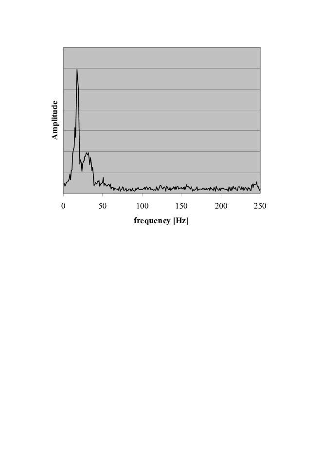
Two analysis methods were used to get the oscillation frequency, both of them from the pick-up coils voltage measurements: spectral analysis, using the Microsoft Excel Fourier analysis instrument (Figure 4 shows a typical example of the spectra we obtained) and the direct measurement on the plot of the oscillation period (“plot method”). The “plot method” has been mainly used as control of the numerical procedure.
The calculated spectra showed various peaks of different amplitude but only the first two in each plot were clearly stronger than the others: see Figure 4. We consistently chose the frequency of the lowest frequency peak as the oscillation frequency of the loop, even in the two cases ( and ) when the two strongest peaks had nearly the same amplitude. The second peak does not usually appear to be harmonic of the first one; we therefore surmise it might be due to the non-uniformity of the field.
The experimental damping time–constant was again obtained in two ways: through the “plot method”, i.e. measuring, from the plots of the pick-up coils voltage, the time it takes for the oscillations to decay to half their initial amplitude, and –when the shape of the main spectral peak was regular enough– through a measure of its half width. As in the previous case, the second method was used for control of the procedure.
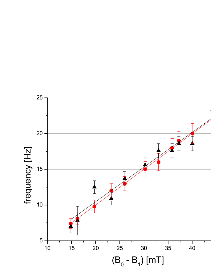
Our results are summarized in Table 1 and Figure 5, where we compare our experimental frequencies to the “theoretical” frequencies, evaluated from equation 7, with calculated as explained above and using the experimental values of The listed error for the “theoretical” frequencies is due to the uncertainties in these two quantities. In particular, for low magnetic fields it is mainly due to the error in the measurements of , while for large magnetic fields it is mainly due to the uncertainty in the value of .
The agreement between the two sets of data in Figure 5 is almost everywhere good; the least square fitting for the experimental data gives a slope of () in good agreement with that obtained from the fitting of the “theoretical” data: ().
| Magnet | Theoretical | Spectrum | analysis | ||
|---|---|---|---|---|---|
| current | model | First | peak | ||
| 0.9 | 14.84 | 7.4 | 0.7 | 7.0 | 0.9 |
| 1.0 | 16.24 | 8.1 | 0.8 | 7.8 | 2.0 |
| 1.25 | 19.74 | 9.8 | 0.9 | 12.5 | 0.9 |
| 1.5 | 23.24 | 12 | 1.0 | 10.9 | 0.9 |
| 1.7 | 26.04 | 13 | 1.0 | 13.7 | 1.0 |
| 2.0 | 30.24 | 15 | 1.1 | 15.6 | 1.0 |
| 2.2 | 33.04 | 16 | 1.2 | 17.6 | 1.0 |
| 2.4 | 35.84 | 18 | 1.3 | 17.6 | 1.0 |
| 2.5 | 37.24 | 19 | 1.3 | 18.6 | 1.0 |
| 2.7 | 40.04 | 20 | 1.4 | 18.6 | 1.0 |
| 3.0 | 44.24 | 22 | 1.5 | 23.4 | 1.0 |
VI Conclusions
Due to easy to perform experiments and the availability of cheap laboratory kits, superconductivity has recently become part of undergraduate lab courses and courses for future physics teachers. Here, we have described a didactic experiment that has the advantage of combining superconductivity with another common lab topic –damped harmonic oscillations– thus giving students the opportunity to deepen their understanding of both. Besides giving the students the chance to tackle many different physics topics such as magnetism, superconductivity, electric currents and oscillations, the experiment we propose involves different detecting devices and data analysis techniques that could easily be presented to students in an almost peer to peer instruction mode.
The experimental data we collected show that the theoretical model we adopted is sufficiently good and that it is therefore suitable for a discussion with college students on superconductivity, Faraday’s law and oscillatory motion based on it and on our experimental set-up. Clearly we could try to improve our model and the fitting of the data but, for that purpose, more refined mathematics should be used and it is our opinion that it could obscure more than lighten the physics involved.
Following the present technical analysis, we are planning to soon report on the in-class experimentation that we are organizing and that will help us decide whether our experiment can help students to get closer to the fascinating phenomena of superconductivity through an “unusual” application.
VII Acknowledgments
We are very grateful to Mr. Castellazzi and Mr. Ormenese of Videotime s.p.a. for their precious help and also to the technicians of L.A.S.A. laboratory for their work and kind suggestions. We also thank Mr. Giuseppe Baccaglioni of L.A.S.A.for having built the pick-up coils and measured the self inductance of the loop.
References
- (1) Several didactic experiments are listed in section VIII-B of N.P. Butch, M.C. de Andrade and M.B. Maple, “Resource Letter Scy-3: Superconductivity”; Am. J. Phys. 76, 106 (2008); http://dx.doi.org/10.1119/1.2802574. More recent papers are e.g.: C.P. Strehlow and M.C. Sullivan, “A classroom demonstration of levitation and suspension of a superconductor over a magnetic track”; Am. J. Phys. 77, 847 (2009); http://dx.doi.org/10.1119/1.3095809, M.R. Osorio, D.E. Lahera and H. Suderow, “Magnetic levitation on a type-I superconductor as a practical demonstration experiment for students”; European Journal of Physics, Volume 33, Number 5, p 1383 (2012), A. Bonanno, G. Bozzo, M. Camarca and P. Sapia, “An innovative experiment on superconductivity, based on video analysis and non-expensive data acquisition”; European Journal of Physics, Volume 36, Number 4, 045010 (2015).
- (2) Several links to providers of kits are available at the “play” page of superconductors.org: http://superconductors.org/play.htm.
- (3) W.Meissner and R. Ochsenfeld, “Ein neuer Effekt bei Eintritt der Supraleitf higkeit”. Naturwissenschaften 21 (44) 787–788 (1933). doi:10.1007/BF01504252.
- (4) D. McAllister, “Magnetic levitation”; Eur. J. Phys., 9, 232-233, 1988.
- (5) R. Romer, “The motion of a superconducting loop in an inhomogeneous magnetic field: the harmonic oscillator equation in an unfamiliar setting”; Eur. J. Phys., 11, 103-106, 1990.