Sensing Hidden Vehicles by Exploiting Multi-Path V2V Transmission

Abstract

This paper presents a technology of sensing hidden vehicles by exploiting multi-path vehicle-to-vehicle (V2V) communication. This overcomes the limitation of existing RADAR technologies that requires line-of-sight (LoS), thereby enabling more intelligent manoeuvre in autonomous driving and improving its safety. The proposed technology relies on transmission of orthogonal waveforms over different antennas at the target (hidden) vehicle. Even without LoS, the resultant received signal enables the sensing vehicle to detect the position, shape, and driving direction of the hidden vehicle by jointly analyzing the geometry (AoA/AoD/propagation distance) of individual propagation path. The accuracy of the proposed technique is validated by realistic simulation including both highway and rural scenarios.

I Introduction

Autonomous driving (auto-driving) is a disruptive technology that will reduce car accidents, traffic congestion, and greenhouse gas emissions by automating the transportation process. One primary operation of auto-driving is vehicular positioning, namely positioning nearby vehicles and even detecting their shapes [1]. The positioning includes both absolute and relative positioning and we focus on relative vehicular positioning in this work. Among others (e.g., cameras and ultrasonic sensing), two existing technologies, namely RADAR and LiDAR (Light Detection and Ranging), are capable of accurate vehicular positioning. RADAR can localize objects as well as estimate their velocities via sending a designed waveform and analyzing its reflection by the objects. Recent breakthroughs in millimeter-wave radar [2] or multiple-input multiple-output (MIMO) radar [3] improves the positioning accuracy substaintially. On the other hand, a LiDAR [4] steers ultra-sharp laser beams to scan the surrounding environment and generate a high resolution three-dimensional (3D) map for navigation. However, RADAR and LiDAR share the common drawback that positioning requires the target vehicles to be visible with line-of-sight (LoS) since neither microwave nor laser beams can penetrate a large solid object such as a truck. Furthermore, hostile weather conditions also affect the effectiveness of LiDAR as fog, snow or rain can severely attenuate a laser beam. On the other hand, detecting hidden vehicles with non-line-of-sight (NLoS) is important for intelligent auto-driving (e.g., overtaking) and accidence avoidance in complex scenarios such as Fig. 1.

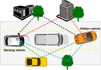
Figure 1: Hidden vehicle scenario with multi-path NLoS channels.

The drawback of existing solutions motivates the current work on developing a technology for sensing hidden vehicles. It relies on V2V transmission to alleviate the severe signal attenuation due to round-trip propagation for RADAR and LiDAR. By designing hidden vehicle sensing, we aim at tackling two main challenges: 1) the lack of LoS and synchronization between sensing and hidden vehicles and 2) simultaneous detection of position, shape, and orientation of driving direction of hidden vehicles.

While LiDAR research focuses on mapping, there exist a rich set of signal processing techniques for positioning using RADAR [5]. They can be largely separated into two themes. The first is time-based ranging by estimating time-of-arrival (ToA) or time-difference-of-arrival (TDoA) [6]. The time-based ranging detects distances but not positions. Most important, the techniques are effective only if there exist LoS paths between sensing and target vehicles. The second theme is positioning using multi-antenna arrays via detecting angle-of-arrival (AoA) and angle-of-departure (AoD) [7]. In addition, there also exist hybrid designs such as jointly using ToA/AoA/AoD [8]. The techniques make the strong assumption that perfect synchronization between transmitters and receivers, which limits their versatility in auto-driving. Furthermore, neither time-based ranging nor array-based positioning is capable of additional geometric information on target vehicles such as their shapes and orientation. In summary, prior designs are insufficient for tackling the said challenges which is the objective of the current work.

The paper presents a technology for hidden vehicle sensing by exploiting multi-path V2V transmission. The technology requires a hidden vehicle to be provision with an array with antennas distributed as multiple clusters over the vehicle body. Furthermore, the vehicle transmits a set of orthogonal waveforms over different antennas. Then by analyzing the multi-path signal observed from a receive array, the geometry (AoA/AoD/propagation distance) of individual path is estimated at the sensing vehicle. Using optimization theory, novel technique is proposed to infer from the multi-path geometric information the position, shape, and orientation of the hidden vehicles. Comprehensive simulation is performed based on practical vehicular channel model including both highway and rural scenarios. Simulation results show the effectiveness of the proposed technology in sensing hidden vehicles.

II System Model

We consider a two-vehicle system where a sensing vehicle (SV) attempts to detect the position, shape, and orientation of a hidden vehicle (HV) blocked by obstacles such as trucks or buildings (see Fig. 1). For the task of only detecting the position and orientation (see Section III), it is sufficient for HV to have an array of collocated antennas (with negligible half-wavelength spacing). On the other hand, for the task of simultaneous detection of position, shape, and orientation (see Section IV), the antennas at the HV are assumed to be distributed as multiple clusters of collocated antennas over HV body. For simplicity, we consider $4$-cluster arrays with clusters at the vertices of a rectangle. Then sensing reduces to detect the positions and shape of the rectangle, thereby also yields the orientation of HV. The relevant technique can be easily extended to a general arrays topology. Last, the SV is provisioned with a $1$-cluster array.

II-A Multi-Path NLoS Channel

The channel between the SV and HV contains NLoS and multi-paths reflected by a set of scatterers. Following the typical assumption for V2V channels, only the received signal from paths with single-reflections is considered at the SV while higher order reflections are neglected due to severe attenuation [9]. Propagation is assumed to be constrained within the horizontal plane to simplify exposition. Consider a 2D Cartesian coordinate system where the SV array is located at the origin and the $X$-axis is aligned with the orientation of SV. Consider a typical $1$-cluster array at the HV. Each NLoS signal path from the HV antenna cluster to the SV array is characterized by the following five parameters (see Fig. 2): the AoA at SV denoted by $\theta$; the AoD at HV denoted by $\varphi$; the orientation of the HV denoted by $\omega$; and the propagation distance denoted by $d$ which includes the propagation distance before refection, denoted by $\nu$, and the remaining distance $d-\nu$. The AoD and AoA are defined as azimuth angles relative to driving directions of HV and SV, respectively.

II-B Hidden Vehicle Transmission

Each of $4$-cluster arrays of HV has $M_{t}$ antennas. The HV is assigned four sets of $M_{t}$ orthogonal waveforms for transmission. Each set is transmitted using a corresponding antennas cluster where each antenna transmits an orthogonal waveform. It is assumed that by network coordinated waveform assignment, HV waveform sets are known at the SV that can hence group the signal paths according their originating antennas clusters arrays. Let $s_{m}(t)$ be the continuous-time baseband waveform assigned to the $m$-th HV antenna with the bandwidth $B_{s}$. Then the waveform orthogonality is specified by $\int s_{m_{1}}(t)s^{*}_{m_{2}}(t)dt=\delta(m_{1}-m_{2})$ with the delta function $\delta(x)=1$ if $x=0$ and $0$ otherwise. The transmitted waveform vector for the $k$-th array of HV antennas cluster is $\mathbf{s}^{(k)}(t)=[s^{(k)}_{1}(t),\cdots,s^{(k)}_{M_{t}}(t)]^{\mathrm{T}}$. With the knowledge of $\{\mathbf{s}^{(k)}(t)\}$, the SV with $M_{r}$ antennas scans and retrieves the receive signal due to the HV transmission.

Consider a typical HV antennas cluster array. Based on the far-field propagation model [10] , the cluster response vector is represented as a function of AoD $\varphi$ as

$$\mathbf{a}(\varphi)=[\exp(j2\pi f_{c}\alpha_{1}(\varphi)),\cdots,\exp(j2\pi f_{c}\alpha_{M_{t}}(\varphi))]^{\mathrm{T}},$$ (1)

where $f_{c}$ denotes the carrier frequency and $\alpha_{m}(\varphi)$ refers to the difference in propagation time to the corresponding scatterer between the $m$-th HV antenna and the $1$-st HV antenna in the same cluster, i.e., $\alpha_{1}(\varphi)=0$. Similarly, the response vector of SV array is expressed in terms of AoA $\theta$ as

$$\mathbf{b}(\theta)=[\exp(j2\pi f_{c}\beta_{1}(\theta)),\cdots,\exp(j2\pi f_{c}\beta_{M_{r}}(\theta))]^{\mathrm{T}},$$ (2)

where $\beta_{m}(\theta)$ refers to the difference of propagation time from the scatterer to the $m$-th SV antenna than the $1$-st SV antenna. We assume that SV has prior knowledge of the response functions $\mathbf{a}(\varphi)$ and $\mathbf{b}(\theta)$. This is feasible by standardizing the vehicular arrays’ topology. In addition, the Doppler effect is ignored based on the assumption that the Doppler frequency shift is much smaller than the waveform bandwidth and thus does not affect waveform orthogonality.

Let $k$ with $1\leq k\leq 4$ denote the index of HV arrays and $P^{(k)}$ denote the number of received paths originating from the $k$-th antennas cluster array. The total number of paths arriving at SV is $P=\sum_{k=1}^{4}P^{(k)}$. Represent the received signal vector at SV as $\mathbf{r}(t)=[r_{1}(t),\cdots,r_{M_{r}}(t)]^{\mathrm{T}}$. It can be expressed in terms of $\mathbf{s}(t)$, $\mathbf{a}(\varphi)$ and $\mathbf{b}(\theta)$ as

$$\mathbf{r}(t)=\sum_{k=1}^{4}\sum_{p=1}^{P^{(k)}}\gamma_{p}^{(k)}\mathbf{b}\left(\theta_{p}^{(k)}\right)\mathbf{a}^{\mathrm{T}}\left(\varphi_{p}^{(k)}\right)\mathbf{s}\left(t-\lambda_{p}^{(k)}\right)+\mathbf{n}(t),$$

where $\gamma_{p}^{(k)}$ and ${\lambda_{p}^{(k)}}$ respectively denote the complex channel coefficient and ToA of path $p$ originating from the $k$-th HV array, and $\mathbf{n}(t)$ represents channel noise. Without synchronization between HV and SV, SV has no information of HV’s transmission timing. Therefore, $\lambda_{p}^{(k)}$ differs from the corresponding propagation delay, denoted by ${\tau_{p}^{(k)}}$, due unknown clock synchronization gap between HV and SV denoted by $\Gamma$. Consequently, $\tau_{p}^{(k)}=\lambda_{p}^{(k)}-\Gamma$.

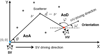
Figure 2: NLoS signal model.

II-C Estimations of AoA, AoD, and ToA

The sensing techniques in the sequel assume that the SV has the knowledge of AoA, AoD, and ToA of each receive NLoS signal path, say path $p$, denoted by $\left\{\theta_{p},\varphi_{p},\lambda_{p}\right\}$ where $p\in\mathcal{P}=\{1,2,\cdots,P\}$. The knowledge can be acquired by applying classical parametric estimation techniques briefly sketched as follows. The estimation procedure comprises the following three steps. 1) Sampling: The received analog signal $\mathbf{r}(t)$ and the waveform vector $\mathbf{s}(t)$ are sampled at the Nyquist rate $2B_{s}$ to give discrete-time signal vectors $\mathbf{r}[n]$ and $\mathbf{s}\left[n\right]$, respectively. 2) Matched filtering: The sequence of $\mathbf{r}[n]$ is matched-filtered using $\mathbf{s}\left[n\right]$. The resultant $M_{r}\times M_{t}$ coefficient matrix $\mathbf{y}[z]$ is given by $\mathbf{y}[z]=\sum_{n}\mathbf{r}[n]\mathbf{s}^{*}\left[n-z\right]$. The sequence of ToAs $\{\lambda_{p}\}$ can be estimated by detecting peaks of the norm of $\mathbf{y}[z]$, denoted by $\{z_{p}\}$, which can be converted into time by multiplying the time resolution $\frac{1}{2B_{s}}$. 3) Estimations of AoA/AoD: Given $\{\mathbf{y}[z_{p}]\}$, AoAs and AoDs are jointly estimated using a 2D-multiple signal classification (MUSIC) algorithm [11]. The estimated AoA $\theta_{p}$, AoD $\varphi_{p}$, ToA $\lambda_{p}$ jointly characterize the $p$-th NLoS path.

II-D Hidden Vehicle Sensing Problem

The SV attempts to sense the HV’s position, shape, and orientation. The position and shape of HV can be obtained by using parameters of AoA $\theta$, AoD $\varphi$, orientation $\omega$, distances $d$ and $\nu$, length and width of configuration of $4$-cluster arrays denoted by $L$ and $W$, respectively. Noting the first two parameters are obtained based on the estimations in Section II-C and the goal is to estimate the remaining five parameters.

III Sensing Hidden Vehicles with Colocated Antennas

Consider the case that the HV has an array with colocated antennas ($1$-cluster array). SV is capable of detecting the HV position, specified by the coordinate ${\mathbf{p}}=(x,y)$, and orientation, specified $\omega$ in Fig. 2. The prior knowledge that the SV has for sensing is the parameters of $P$ NLoS paths estimated as described in Section II-C. Each path, say path $p$, is characterized by the parametric set $\{\theta_{p},\varphi_{p},\lambda_{p}\}$. Then the sensing problem in the current case can be represented as

$$\quad\bigcup_{p\in\mathcal{P}}\{\theta_{p},\varphi_{p},\lambda_{p}\}\Rightarrow\{{\mathbf{p}},\omega\}.$$ (3)

The problem is solved in the following subsections.

III-A Sensing Feasibility Condition

In this subsection, it is shown that for the sensing to be feasible, there should exist at least four NLoS paths. To this end, based on the path geometry (see Fig. 2), we can obtain the following system of equations:

$$\begin{cases}x_{p}=\nu_{p}\cos(\theta_{p})-(d_{p}-\nu_{p})\cos(\varphi_{p}+\omega)\\ =\nu_{1}\cos(\theta_{1})-(d_{1}-\nu_{1})\cos(\varphi_{1}+\omega),\\ y_{p}=\nu_{p}\sin(\theta_{p})-(d_{p}-\nu_{p})\sin(\varphi_{p}+\omega)\\ =\nu_{1}\sin(\theta_{1})-(d_{1}-\nu_{1})\sin(\varphi_{1}+\omega),\end{cases}p\in\mathcal{P}.$$ (P1)

The number of equations in P1 is $2(P-1)$, and the above system of equations has a unique solution when the dimensions of unknown variables are less than $2(P-1)$. Since the AoAs $\{\theta_{p}\}$ and AoDs $\{\varphi_{p}\}$ are known, the number of unknowns is $(2P+1)$ including the propagation distances $\{d_{p}\}$, $\{\nu_{p}\}$, and orientation $\omega$. To further reduce the number of unknowns, we use the propagation time difference between signal paths also known as TDoAs, denoted by $\{\rho_{p}\}$, which can be obtained from the difference of ToAs as $\rho_{p}=\lambda_{p}-\lambda_{1}$ where $\rho_{1}=0$. The propagation distance of signal path $p$, say $d_{p}$, is then expressed in terms of $d_{1}$ and $\rho_{p}$ as

$$d_{p}=c(\lambda_{p}-\Gamma)=c(\lambda_{1}-\Gamma)+c(\lambda_{p}-\lambda_{1})=d_{1}+c\rho_{p},$$ (4)

for $p=\{2,\cdots,P\}$. Substituting the above $(P-1)$ equations into P1 eliminates the unknowns $\{d_{2},\cdots,d_{P}\}$ and hence reduces the number of unknowns from $(2P+1)$ to $(P+2)$. As a result, P1 has a unique solution when $2(P-1)\geq P+2$.

Proposition 1 (Sensing feasibility condition).

To sense the position and orientation of a HV with $1$-cluster array, at least four NLoS signal paths are required: $P\geq 4$.

Remark 1 (Asynchronization and TDoA).

Recall that one sensing challenge is asynchronization between HV and SV represented by $\Gamma$, which is a latent variable we cannot observe explicitly. Considering TDoA helps solve the problem by avoiding the need of considering $\Gamma$ by exploiting the fact that all NLoS paths experience the same synchronization gap.

III-B Hidden Vehicle Sensing without Noise

Consider the case of a high receive signal-to-noise ratio (SNR) where noise can be neglected. Then the sensing problem in (3) is translated to solve the system of equations in P1. One challenge is that the unknown orientation $\omega$ introduces nonlinear relations, namely $\cos(\varphi_{p}+\omega)$ and $\sin(\varphi_{p}+\omega)$, in the equations. To overcome the difficulty, we adopt the following two-step approach: 1) Estimate the correct orientation $\omega^{*}$ via its discriminant introduced in the sequel; 2) Given $\omega^{*}$, the equations becomes linear and thus can be solved via least-square (LS) estimator, giving the position ${\mathbf{p}}^{*}$. To this end, the equations in P1 can be arranged in a matrix form as

$$\mathbf{A}(\omega)\mathbf{z}=\mathbf{B}(\omega),$$ (P2)

where $\mathbf{z}=(\mathbf{v},d_{1})^{\mathrm{T}}\in\mathds{R}^{(P+1)\times 1}$ and $\mathbf{v}=\{\nu_{1},\cdots,\nu_{P}\}$. For matrix $\mathbf{A}(\omega)$, we have

$$\mathbf{A}(\omega) =\begin{bmatrix}\mathbf{A}^{(\cos)}(\omega)\\ \mathbf{A}^{(\sin)}(\omega)\end{bmatrix}\in\mathds{R}^{2(P-1)\times(P+1)},$$ (5)

where $\mathbf{A}^{(\cos)}(\omega)$ is

$$\begin{bmatrix}a_{1}^{(\cos)}&-a_{2}^{(\cos)}&0&\cdots&0&a_{1,2}^{(\cos)}\\ a_{1}^{(\cos)}&0&-a_{3}^{(\cos)}&\cdots&0&a_{1,3}^{(\cos)}\\ \vdots&\vdots&\vdots&\ddots&\vdots&\vdots\\ a_{1}^{(\cos)}&0&0&\cdots&-a_{P}^{(\cos)}&a_{1,P}^{(\cos)}\\ \end{bmatrix}$$ (6)

with $a_{p}^{(\cos)}=\cos(\theta_{p})+\cos(\varphi_{p}+\omega)$ and $a_{1,p}^{(\cos)}=\cos(\varphi_{p}+\omega)-\cos(\varphi_{1}+\omega)$, and $\mathbf{A}^{(\sin)}(\omega)$ is obtained by replacing all $\cos$ operations in (6) with $\sin$ operations. Next,

$$\mathbf{B}(\omega)=\begin{bmatrix}\mathbf{B}^{(\cos)}(\omega)\\ \mathbf{B}^{(\sin)}(\omega)\end{bmatrix}\in\mathds{R}^{2(P-1)\times 1},$$ (7)

where

$$\mathbf{B}^{(\cos)}(\omega)=\begin{bmatrix}c\rho_{2}\cos(\varphi_{2}+\omega)\\ c\rho_{3}\cos(\varphi_{3}+\omega)\\ \vdots\\ c\rho_{P}\cos(\varphi_{P}+\omega)\\ \end{bmatrix},$$ (8)

and $\mathbf{B}^{(\sin)}(\omega)$ is obtained by replacing all $\cos$ in (8) with $\sin$.

1) Computing $\omega^{*}$: Note that P2 becomes an over-determined linear system of equations if $P\geq 4$ (see Proposition 1), providing the following discriminant of orientation $\omega$. Since the equations in (5) are based on the geometry of multi-path propagation and HV orientation as illustrated in Fig. 2, there exists a unique solution for the equations. Then we can obtain from (5) the following result useful for computing $\omega^{*}$.

Proposition 2 (Discriminant of orientation).

With $P\geq 4$, a unique $\omega^{*}$ exists when $\mathbf{B}(\omega^{*})$ is orthogonal to the null column space of $\mathbf{A}(\omega^{*})$ denoted by $\mathsf{null}(\mathbf{A}(\omega^{*})^{\mathrm{T}})\in\mathds{R}^{2(P-1)\times(P-3)}$:

$$\mathsf{null}(\mathbf{A}(\omega^{*})^{\mathrm{T}})^{\mathrm{T}}\mathbf{B}(\omega^{*})=\mathbf{0}.$$ (9)

Given this discriminant, a simple 1D search can be performed over the range $[0,2\pi]$ to find $\omega^{*}$.

2) Computing ${\mathbf{p}}^{*}$: Given the $\omega^{*}$, P2 can be solved by

$$\mathbf{z}^{*}=\left[\mathbf{A}(\omega^{*})^{\mathrm{T}}\mathbf{A}(\omega^{*})\right]^{-1}\mathbf{A}(\omega^{*})^{\mathrm{T}}\mathbf{B}(\omega^{*}).$$ (10)

Then the estimated HV position ${\mathbf{p}}^{*}$ can be computed by substituting (9) and (10) into (4) and P1.

III-C Hidden Vehicle Sensing with Noise

In the presence of significant channel noise, the estimated AoAs/AoDs/ToAs contain errors. Consequently, HV sensing is based on the noisy versions of matrix $\mathbf{A}(\omega)$ and $\mathbf{B}(\omega)$, denoted by $\tilde{\mathbf{A}}(\omega)$ and $\tilde{\mathbf{B}}(\omega)$, which do not satisfy the equations in P2 and (9). To overcome the difficulty, we develop a sensing technique by converting the equations into minimization problems whose solutions are robust against noise.

1) Computing $\omega^{*}$: Based on (9), we formulate the following problem for finding the orientation $\omega$:

$$\omega^{*}=\arg\min_{\omega}\left[\mathsf{null}(\tilde{\mathbf{A}}(\omega)^{\mathrm{T}})^{\mathrm{T}}\tilde{\mathbf{B}}(\omega)\right].$$ (11)

Solving the problem relies on a 1D search over $[0,2\pi]$.

2) Computing ${\mathbf{p}}^{*}$: Next, given $\omega^{*}$, the optimal $\mathbf{z}^{*}$ can be derived by using the LS estimator that minimizes the squared Euclidean distance as

$$\mathbf{z}^{*} =\arg\min_{\mathbf{z}}\|\tilde{\mathbf{A}}(\omega^{*})\mathbf{z}-\tilde{\mathbf{B}}(\omega^{*})\|^{2}$$

$$=\left[\tilde{\mathbf{A}}(\omega^{*})^{\mathrm{T}}\tilde{\mathbf{A}}(\omega^{*})\right]^{-1}\tilde{\mathbf{A}}(\omega^{*})^{\mathrm{T}}\tilde{\mathbf{B}}(\omega^{*}),$$ (12)

which has the same structure as (10). Last, the origins of all paths $\{(x_{p},y_{p})\}_{p\in\mathcal{P}}$ can be computed using the parameters $\{\mathbf{z}^{*},\omega^{*}\}$ as illustrated in P1. Averaging these origins gives the estimate of the HV position ${\mathbf{p}}^{*}=(x^{*},y^{*})$ with $x^{*}=\frac{1}{P}\sum_{p=1}^{P}x_{p}$ and $y^{*}=\frac{1}{P}\sum_{p=1}^{P}y_{p}$.

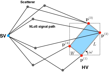
Figure 3: Rectangular configuration of $4$-cluster arrays at HV.

IV Sensing Hidden Vehicles with Multi-Cluster Arrays

Consider the case that the HV arrays consists of four antenna clusters located at the vertices of a rectangle with length $L$ and width $W$ (see Fig. 3). The vertex locations are represented as $\{{\mathbf{p}}^{(k)}=(x^{(k)},y^{(k)})^{\mathrm{T}}\}_{k=1}^{4}$. Recall that the SV can differentiate the origin from which signal is transmitted due to the usage of different orthogonal waveform set for each array. Let each path be ordered based on HV arrays’ index such that $\mathcal{P}=\{\mathcal{P}^{(1)},\mathcal{P}^{(2)},\mathcal{P}^{(3)},\mathcal{P}^{(4)}\}$ where $\mathcal{P}^{(k)}$ represents the set of received signals from the $k$-th array. Note that the vertices determines the shape and their centroid of HV location. Therefore, the sensing problem is represented as

$$\bigcup\nolimits_{k=1}^{4}\bigcup\nolimits_{p\in\mathcal{P}^{(k)}}\{\theta_{p},\varphi_{p},\lambda_{p}\}\Rightarrow\{\{{\mathbf{p}}^{(k)}\}_{k=1}^{4},\omega\}.$$ (13)

Next, we present a sensing technique exploiting prior knowledge of the HV $4$-cluster arrays’ configuration, which is more efficient than separately estimating the four positions $\{{\mathbf{p}}^{(k)}\}_{k=1}^{4}$ using the technique in the preceding section.

IV-A Sensing Feasibility Condition

Assume that $\mathcal{P}^{(1)}$ is not empty and $1\in\mathcal{P}^{(1)}$ without loss of generality. Based on the rectangular configuration of $\{\mathbf{p}^{(k)}\}_{k=1}^{4}$ (see Fig. 3), a system of equations is formed:

$$\!\!\!\!\begin{cases}\nu_{p}\cos(\theta_{p})-(d_{p}-\nu_{p})\cos(\varphi_{p}+\omega)+\eta_{p}(\omega,L,W)\\ =\nu_{1}\cos(\theta_{1})-(d_{1}-\nu_{1})\cos(\varphi_{1}+\omega),\\ \nu_{p}\sin(\theta_{p})-(d_{p}-\nu_{p})\sin(\varphi_{p}+\omega)+\zeta_{p}(\omega,L,W)\\ =\nu_{1}\sin(\theta_{1})-(d_{1}-\nu_{1})\sin(\varphi_{1}+\omega),\end{cases}$$ (P3)

where

$$\eta_{p}(\omega,L,W)=\left\{\begin{aligned} &0,&&\textrm{$p\in\mathcal{P}^{(1)}$}\\ &L\cdot\cos(\omega),&&\textrm{$p\in\mathcal{P}^{(2)}$}\\ &L\cdot\cos(\omega)-W\cdot\sin(\omega),&&\textrm{$p\in\mathcal{P}^{(3)}$}\\ &-W\cdot\sin(\omega),&&\textrm{$p\in\mathcal{P}^{(4)}$}\end{aligned}\right.$$ (14)

and $\zeta_{p}(\omega,L,W)$ is obtained via replacing all $\cos$ and $\sin$ in $\eqref{funcLW1}$ with $\sin$ and $-\cos$, respectively. Recall $P=|\mathcal{P}|=\sum_{k=1}^{4}|\mathcal{P}^{(k)}|$. Compared with P1, the number of equations in P3 is the same as $2(P-1)$ while the number of unknowns increases from $P+2$ to $P+4$ because $L$ and $W$ are also unknown. Consequently, P3 has a unique solution when $2(P-1)\geq P+4$.

Proposition 3 (Sensing feasibility condition).

To sense the position, shape, and orientation of a HV with $4$-cluster arrays, at least six paths are required: $P\geq 6$.

Remark 2 (Advantage of array-configuration knowledge).

The separate positioning of individual HV $4$-cluster arrays requires at least $16$ NLoS paths (see Proposition 1). On the other hand, the prior knowledge of rectangular configuration of antenna clusters leads to the relation between their locations, reducing the number of required paths for sensing.

IV-B Hidden Vehicle Sensing

Consider the case that noise is neglected. P2 is rewritten to the following matrix form:

$$\hat{\mathbf{A}}(\omega)\hat{\mathbf{z}}={\mathbf{B}}(\omega),$$ (P4)

where $\hat{\mathbf{z}}=(\mathbf{v},d_{1},L,W)^{\mathrm{T}}\in\mathds{R}^{(P+3)\times 1}$ with $\mathbf{v}$ following the index ordering of $\mathcal{P}$, and ${\mathbf{B}}(\omega)$ is given in (7). For matrix $\hat{\mathbf{A}}(\omega)$, we have

$$\hat{\mathbf{A}}(\omega) =\begin{bmatrix}\mathbf{A}(\omega)&\mathbf{L}(\omega)&\mathbf{W}(\omega)\end{bmatrix}\in\mathds{R}^{2(P-1)\times(P+3)}.$$ (15)

Here, $\mathbf{A}(\omega)$ is specified in (5) and $\mathbf{L}(\omega)\in\mathds{R}^{2(P-1)\times 1}$ is given as $[\mathbf{L}^{(\cos)}(\omega),\mathbf{L}^{(\sin)}(\omega)]^{\mathrm{T}}$ where

$$\mathbf{L}^{(\cos)}(\omega) =[\underbrace{0,\cdots,0}_{|\mathcal{P}^{(1)}|-1},\underbrace{-\cos(\omega),\cdots,-\cos(\omega)}_{|\mathcal{P}^{(2)}|+|\mathcal{P}^{(3)}|},\underbrace{0,\cdots,0}_{|\mathcal{P}^{(4)}|}]^{\mathrm{T}},$$

and $\mathbf{L}^{(\sin)}(\omega)$ is obtained by replacing all $\cos(\omega)$ in $\mathbf{L}^{(\cos)}(\omega)$ with $\sin(\omega)$. Similarly, $\mathbf{W}(\omega)$ is given as $[\mathbf{W}^{(\sin)}(\omega),\mathbf{W}^{(\cos)}(\omega)]^{\mathrm{T}}$ where

$$\mathbf{W}^{(\sin)}(\omega) =[\underbrace{0,\cdots,0}_{|\mathcal{P}^{(1)}|+|\mathcal{P}^{(2)}|-1},\underbrace{\sin(\omega),\cdots,\sin(\omega)}_{|\mathcal{P}^{(3)}|+|\mathcal{P}^{(4)}|}]^{\mathrm{T}},$$

and $\mathbf{W}^{(\cos)}(\omega)$ is obtained by replacing all $\sin$ in $\mathbf{W}^{(\sin)}(\omega)$ with $-\cos$.

1) Computing $\omega^{*}$: Noting that P4 is over-determined when $P\geq 6$, the resultant discriminant of the orientation $\omega$ is similar to Proposition 2 and given as follows.

Proposition 4 (Discriminant of orientation).

With $P\geq 6$, the unique $\omega^{*}$ exists when $\hat{\mathbf{B}}(\omega^{*})$ is orthogonal to the null column space of $\hat{\mathbf{A}}(\omega^{*})$ denoted by $\mathsf{null}(\hat{\mathbf{A}}(\omega^{*})^{\mathrm{T}})\in\mathds{R}^{2(P-1)\times(P+1)}$:

$$\mathsf{null}(\hat{\mathbf{A}}(\omega^{*})^{\mathrm{T}})^{\mathrm{T}}\hat{\mathbf{B}}(\omega^{*})=\mathbf{0}.$$ (16)

Given this discriminant, a simple 1D search can be performed over the range $[0,2\pi]$ to find $\omega^{*}$.

2) Computing $\{{\mathbf{p}}^{(k)}\}_{k=1}^{4}$: Given the $\omega^{*}$, P4 can be solved by

$$\hat{\mathbf{z}}^{*}=\left[\hat{\mathbf{A}}(\omega^{*})^{\mathrm{T}}\hat{\mathbf{A}}(\omega^{*})\right]^{-1}\hat{\mathbf{A}}(\omega^{*})^{\mathrm{T}}\hat{\mathbf{B}}(\omega^{*}).$$ (17)

HV arrays’ positions $\{{\mathbf{p}}^{(k)}\}_{k=1}^{4}$ can be computed by substituting (16) and (17) into (4) and P3.

Extending the technique to the case with noise is omitted for brevity because it is straightforward by modifying (16) to a minimization problem as in Sec. III-C.

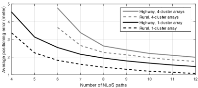
Figure 4: Number of NLoS paths versus average positioning error.

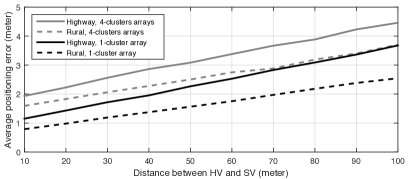
Figure 5: SV-HV distance versus average positioning error.

V Simulation Results

The performance of the proposed technique is validated via realistic simulation. The performance metric for measuring positioning accuracy is defined as the average Euclidean squared distance of estimated arrays’ positions to their true locations: $\frac{1}{4}\sum_{k=1}^{4}\|{\mathbf{p}}^{*(k)}-{\mathbf{p}}^{(k)}\|^{2}$, named average positioning error. We adopt the geometry-based stochastic channel model given in [12] for modelling the practical scatterers distribution and V2V propagation channels, which has been validated by real measurement data. Two scenarios, highway and rural, are considered by following the settings in [12, Table 1]. We set $f_{c}=5.9$ GHz, $B_{s}=100$ MHz, $M_{r}=M_{t}=20$, the per-antenna transmission power is $23$ dBm. The size of HV is $L\times W=3\times 6\leavevmode\nobreak\ \textrm{m}^{2}$ and distance between SV and HV is $50\leavevmode\nobreak\ \textrm{m}$.

Fig. 4 shows the curves of average positioning error versus the number of NLoS paths $P$ received at SV. It is observed that positioning via $1$ and $4$-cluster arrays are feasible when the $P\geq 4$ and $P\geq 6$, respectively, and receiving more paths can dramatically decrease the positioning error. The error for the $4$-cluster arrays is much larger. This is because more clusters results in more noise, which leads to noisy estimations of AoA/AoD/ToAs within signal detection procedure. Also, compared with $1$-cluster array, two more unknown parameters need to be jointly estimated in the case of $4$-cluster arrays, which impacts the positioning performance. Moreover, the positioning accuracy in the rural scenario is better than that in highway scenario. The reason is that the signal propagation loss in highway scenario is higher than that in rural scenario since the distance between vehicle and scatterers can be large, which adds the difficulty for signal detections.

In Fig. 5, the distance between SV and HV versus average positioning error is plotted. It is shown that the positioning error increases when SV-HV distance keeps increasing because the accuracy of signal detection reduces when SV-HV distance becomes larger since higher signal propagation loss. The positioning accuracy in rural scenario is higher than that in highway. The reason is that more paths can be received at SV in rural case due to the denser scatterers exists, resulting in higher positioning accuracy as Fig. 4 displays. Moreover, the error gap between highway and rural cases increases with SV-HV distance. This is because, as the SV-HV distance increases, the power of received signals in highway is weaker than those in rural due to larger propagation loss, leading to inaccurate signal detections.

VI Conclusion Remarks

A novel and efficient technique has been proposed for sensing hidden vehicles. Presently, we are extending the technique to the case where the SV has no knowledge of waveform assignments to different HV arrays, and to 3D propagation.

References

- [1] N. Alam and A. Dempster, “Cooperative positioning for vehicular networks: Facts and future,” IEEE Trans. Intell. Transp. Syst., vol. 14, pp. 1708–1717, Dec. 2013.
- [2] J. Choi and et al., “Millimeter-wave vehicular communication to support massive automotive sensing,” IEEE Commun. Mag., vol. 54, pp. 160–167, Dec. 2016.
- [3] M. Rossi, A. Haimovich, and Y. Eldar, “Spatial compressive sensing for mimo radar,” IEEE Trans. Sig. Proc., vol. 62, pp. 419–430, Jan. 2014.
- [4] B. Schwarz, “Lidar: Mapping the world in 3d,” Nature Photonics, vol. 4, pp. 429–430, Jul. 2010.
- [5] S. Gezici and et al, “Localization via ultra-wideband radios: a look at positioning aspects for future sensor networks,” IEEE Signal Proc. Mag., vol. 22, pp. 70–84, Jul. 2005.
- [6] D.-H. Shin and T.-K. Sung, “Comparisons of error characteristics between toa and tdoa positioning,” IEEE Trans Aerospace Elec. Systems, vol. 38, pp. 307–311, Jan. 2002.
- [7] H. Miao, K. Yu, and M. J. Juntti, “Positioning for NLOS propagation: Algorithm derivations and Cramer-Rao bounds,” IEEE Trans. Veh. Tech., vol. 56, pp. 2568–2580, Sep. 2007.
- [8] A. Shahmansoori and et al, “Position and orientation estimation through millimeter-wave MIMO in 5G systems,” IEEE Trans. Wireless Commun., vol. 17, pp. 1822–1835, Mar. 2018.
- [9] L. Cheng, D. Stancil, and F. Bai, “A roadside scattering model for the vehicle-to-vehicle communication channel,” IEEE J. Sel. Areas Commun., vol. 31, pp. 449–459, Sep. 2013.
- [10] X. Cui, T. Gulliver, J. Li, and H. Zhang, “Vehicle positioning using 5G Millimeter-wave systems,” IEEE Access, vol. 4, pp. 6964–6973, Oct. 2016.
- [11] C. Mathews and M. Zoltowski, “Eigenstructure techniques for 2-D angle estimation with uniform circular arrays,” IEEE Trans. Sig. Proc., vol. 42, pp. 2395–2407, Sep. 1994.
- [12] J. Karedal and et al., “A geometry-based stochastic MIMO model for vehicle-to-vehicle communications,” IEEE Trans. Wireless Commun., vol. 8, pp. 3646–3657, Jul. 2009.