Hamiltonian Monte Carlo for Probabilistic Programs with Discontinuities

Abstract.

Hamiltonian Monte Carlo (HMC) is arguably the dominant statistical inference algorithm used in most popular “first-order differentiable” Probabilistic Programming Languages (PPLs). However, the fact that HMC uses derivative information causes complications when the target distribution is non-differentiable with respect to one or more of the latent variables.

In this paper, we show how to use extensions to HMC to perform inference in probabilistic programs that contain discontinuities. To do this, we design a Simple first-order Probabilistic Programming Language (SPPL) that contains a sufficient set of language restrictions together with a compilation scheme. This enables us to preserve both the statistical and syntactic interpretation of if-else statements in the probabilistic program, within the scope of first-order PPLs. We also provide a corresponding mathematical formalism that ensures any joint density denoted in such a language has a suitably low measure of discontinuities.

1. Introduction

Hamiltonian Monte Carlo (HMC) (Duane et al., 1987; Neal, 2011) is an efficient Markov Chain Monte Carlo (MCMC) algorithm that has been widely used for inference in a wide-range of probabilistic models (Jacobs et al., 2016; Svensson et al., 2017; Doyle et al., 2016). Its superior performance arises from the advantageous properties of the sample paths that it generates via Hamiltonian mechanics. HMC, particularly the No-U-turn sampler (NUTS) (Hoffman and Gelman, 2014) variant, is implemented in many Probabilistic Programming Systems (PPSs)(Eli et al., 2017; Tran et al., 2017; Salvatier et al., 2016; Gelman et al., 2015), and is the main inference engine of both PyMC3 (Salvatier et al., 2016) and Stan (Gelman et al., 2015; Carpenter et al., 2015).

One drawback of using HMC in probabilistic programming is that complications can arise when the target distribution is not differentiable with respect to one or more of its parameters. Developers often impose restrictions on the models that can be encoded to try and avoid these complications, such as preventing the use of discrete variables or only allowing them if they are directly marginalized out.

However, even these restrictions are not sufficient to guarantee the program is discontinuity-free because control flow special forms, such as if-else statements in PPLs, can also induce discontinuities.

Though it turns out, perhaps surprisingly, that HMC still constitutes a valid inference algorithm when the target is discontinuous or even if it has disjoint support, this can substantially reduce the acceptance rate leading to inefficient inference.

To mitigate this issue, several variants of HMC have been developed (Afshar and Domke, 2015; Nishimura et al., 2017) to perform inference on models with discontinuous densities. However, existing systems, like Stan, are not able to support these variants as their compilation procedures do not unearth the required discontinuity information. Creating a system that addresses this issue in an automated way is non-trivial and requires significant heavy lifting from the programming languages perspective.

Therefore, in this extended abstract, we define a carefully designed probabilistic programming language with an accompanying denotational semantics and compiler. Together, these are able to both recover the discontinuity information required to use these HMC variants as inference engines and provide a framework amenable to the theoretical analysis required to demonstrate the correctness of the resulting engines. To ensure that the measure of the set of discontinuities in the target density is of measure zero, we provide a mathematical formalism to compliment our language. This then provides us with a framework in which we can conservatively and correctly employ HMC and its variants. We demonstrate this for the Discontinuous Hamiltonian Monte Carlo  (DHMC) algorithm (Nishimura et al., 2017) and provide an example of our language being employed on models that have non-differentiable densities.

2. A Simple PPL

SPPL uses a Lisp style syntax, like that of Church (Goodman et al., 2008), Anglican (Wood et al., 2014) and Venture (Mansinghka et al., 2014). The syntax of expressions $e$ in our language is given as follows:

$${{{{\begin{array}[]{@{}r@{}c@{}l@{}}e&\,::=&x\mid c\mid\,(p\ e\,\ldots\,e)\,\mid\,(\texttt{\leavevmode\lstinline{{\lst@@@set@language\lst@@@set@numbers\lst@@@set@frame\lst@@@set@rulecolor\lst@@@set@language\lst@@@set@language\scriptsize{\@listingGroup{ltx_lst_keywords3}{\color[rgb]{0.60,0.0,0.0}if}}}}}}\ (<e\ 0)\ e\ e)\,\mid\,(\texttt{\leavevmode\lstinline{{\lst@@@set@language\lst@@@set@numbers\lst@@@set@frame\lst@@@set@rulecolor\lst@@@set@language\lst@@@set@language\scriptsize{\@listingGroup{ltx_lst_keywords3}{\color[rgb]{0.60,0.0,0.0}let}}}}}}\ [x\ e]\ e)\\ &\,\mid&(\texttt{\leavevmode\lstinline{{\lst@@@set@language\lst@@@set@numbers\lst@@@set@frame\lst@@@set@rulecolor\lst@@@set@language\lst@@@set@language\scriptsize{\@listingGroup{ltx_lst_keywords8}{\color[rgb]{0,0.3,0.7}sample}}}}}}\ (d\ e\,\ldots\,e))\,\mid\,(\texttt{\leavevmode\lstinline{{\lst@@@set@language\lst@@@set@numbers\lst@@@set@frame\lst@@@set@rulecolor\lst@@@set@language\lst@@@set@language\scriptsize{\@listingGroup{ltx_lst_keywords8}{\color[rgb]{0,0.3,0.7}observe}}}}}}\ (d\ e\,\ldots\,e)\ c)\vspace{-5pt}\end{array}$$

We use $x$ for a real-valued variable, $c$ for a real number, $p$ for an analytic primitive operation on real, such as $+$ and $\exp{}$, and $d$ for the type of a distribution on $\mathbb{R}$, such as Normal, that has a piece-wise smooth density under analytic partition.

To be less technical, this is restricted on $d$ only allows continuous distribution as primitives. However, one can easily construct discrete distributions as was seen in Figure 1, where Program 1 (a) and 2 (b) define the joint density of the model respectively as following,

$$p_{1}(z,y)= \,p_{B}(z;q)\,p_{\mathcal{N}}(y;1,1)^{\mathbb{I}(z=1)}\,p_{\mathcal{N}}(y;0,1)^{\mathbb{I}(z=0)}$$

$$p_{2}(x,y)= \,p_{U}(x;0,1)\,p_{\mathcal{N}}(y;1,1)^{\mathbb{I}(x>q)}\,p_{\mathcal{N}}(y;0,1)^{\mathbb{I}(x\leq q)}$$

Note that there are no forms for applying general functions in this language and no recursion is possible at all. As a result, all programs written in this language may only have a finite and fixed number of sample and observe statements. This means, among other things, that programs in this language can be compiled to graphical models in which there are finite number of random variable vertices coming from every sample and observe statement. For this reason we will mix our use of the terms graphical model and probabilistic program, or just program, because of their equivalence.

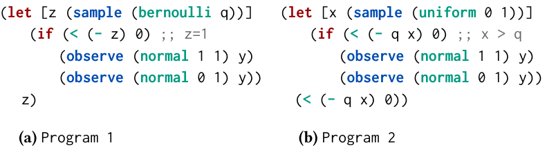
Figure 1. A simple probabilistic program example written in Anglican (a) with Bernoulli distribution as a primitive and an equivalent one in SPPL (b) where the Bernoulli draw is constructed by a Uniform-draw and if-else statement.

The primitives are, by design, restricted to be analytic. Analytic functions are abundant and most primitive functions that we encounter in machine learning applications are analytic, and their composition is also analytic.

Intuitively, programs in SPPL have a joint density in the form as Definition 1 (See Appendix A). It can be understood as a collection of smooth functions in each partition, with no partition overlapping and the union of all partitions is the total space $\mathbb{R}^{k}$. To evaluate the sum, therefore, we just need to evaluate these products at $x$ one-by-one until we find one that returns a non-zero value. Then, we have to compute the function $\color[rgb]{0,0,0}h_{i}$ corresponding to this product at the input $x$.

Theorem 1.

If the density $f:\mathbb{R}^{n}\to\mathbb{R}_{+}$ has the form of Definition 1 and so is piecewise smooth under analytic partition, then there exists a (Borel) measurable subset $A\subseteq\mathbb{R}^{n}$ such that $f$ is differentiable outside of $A$ and the Lebesgue measure of $A$ is zero.

Together with Definition 1 and Theorem 1, we ensures that SPPL conforms to Lemma 1 and Theorems 2 and 3 of DHMC (Nishimura et al., 2017) and so, by design, all requirements for DHMC are trivially met as the density is a piecewise smooth function and all discontinuities are of measure zero.

3. The Compilation Scheme

Accompanying the language, our compilation scheme is designed to establish variables which the density is discontinuous with respect to and provide information for runtime checking on boundary crossing. It works by automatically extracting if predicates and evaluating them with the corresponding random variables. Each predicate is assigned a unique name and corresponding boolean. If the boolean changes value, it indicates the corresponding random variable has crossed the boundary during the update in inference at runtime. The runtime checker will record this information and pass it to the inference engine. Note that the runtime checking can only detect boundary crossing instead of being able to calculate the analytical solution on where the boundaries are exactly. We recognize the former part is sufficient for many specialized inference engines and leave the later part to be implemented as future work.

4. Experiment

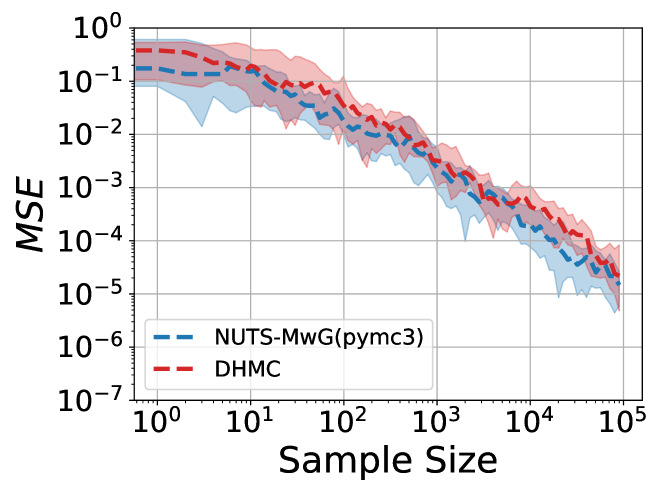
Figure 2. Mean Squared Error for the posterior estimates to true posterior of the cluster means $\mu_{1:2}$. We compare the results from DHMC and NUTS with Metropolis-within-Gibbs(MwG). The median (dashed lines) and $20\%/80\%$ confidence intervals(shaded) over $20$ independent runs are shown.

We now consider a classic Gaussian mixture model (GMM), where one is interested to estimate the mean of each cluster and the cluster assignment for each data. The density of this model contains a mixture of continuous and discrete variables (See details of the model in Appendix C).

We compared the Mean Squared Error (MSE) of the posterior estimates for the cluster means of both an unoptimized version of DHMC and PyMC3 (Salvatier et al., 2016) optimized implementation of NUTS with Metropolis-within-Gibbs(MwG), with the same computation budget. The results are shown in Figure 2 as a function of number of samples. We take $100,000$ samples and discard $10,000$ for burn in. We calculate the $20\%/80\%$ confidence intervals over 20 independent runs and find that both approaches perform consistently well. We find that our unoptimized DHMC implementation, performs comparable to the optimized NUTS with MwG approach.

Appendix A Piecewise Smooth Function

Definition 1.

A function $f:\mathbb{R}^{k}\to\mathbb{R}$ is piecewise smooth under analytic partition if it has the following form:

$$\color[rgb]{0,0,0}f(\color[rgb]{0,0,0}x\color[rgb]{0,0,0})\color[rgb]{0,0,0}=\sum_{i=1}^{N}\left(\prod_{j=1}^{M_{i}}\mathbb{I}(\color[rgb]{0,0,0}p_{i,j}\color[rgb]{0,0,0}(\color[rgb]{0,0,0}x\color[rgb]{0,0,0})\geq\color[rgb]{0,0,0}0)\color[rgb]{0,0,0}\cdot\prod_{l=1}^{O_{i}}\mathbb{I}(\color[rgb]{0,0,0}q_{i,l}\color[rgb]{0,0,0}(\color[rgb]{0,0,0}x\color[rgb]{0.60,0.0,0.0}\color[rgb]{0,0,0})<\color[rgb]{0,0,0}0)\cdot\color[rgb]{0,0,0}h_{i}(\color[rgb]{0,0,0}x\color[rgb]{0,0,0})\right)$$

where

1. the $\color[rgb]{0,0,0}p_{i,j},q_{i,l}\color[rgb]{0,0,0}:\mathbb{R}^{k}\to\mathbb{R}$ are analytic;

2. the $\color[rgb]{0,0,0}h_{i}\color[rgb]{0,0,0}:\mathbb{R}^{k}\to\mathbb{R}$ are smooth;

3. $N$ is a non-negative integer or $\infty$;

4. $M_{i},O_{i}$ are non-negative integers; and

5. the indicator functions

   $$\prod_{j=1}^{M_{i}}\mathbb{I}(\color[rgb]{0,0,0}p_{i,j}\color[rgb]{0,0,0}(\color[rgb]{0,0,0}x\color[rgb]{0,0,0})\geq\color[rgb]{0,0,0}0)\color[rgb]{0,0,0}\cdot\prod_{l=1}^{O_{i}}\mathbb{I}(\color[rgb]{0,0,0}q_{i,l}\color[rgb]{0,0,0}(\color[rgb]{0,0,0}x\color[rgb]{0.60,0.0,0.0}\color[rgb]{0,0,0})<\color[rgb]{0,0,0}0)\cdot\color[rgb]{0,0,0}h_{i}(\color[rgb]{0,0,0}x\color[rgb]{0,0,0})$$

   for the indices $i$ define a partition of $\mathbb{R}^{k}$ as,

   $$\left\{\left\{x\,{\in}\,\mathbb{R}^{k}\;\Big{|}\;\begin{array}[]{@{}l@{}}\color[rgb]{0,0,0}p_{i,j}\color[rgb]{0,0,0}(\color[rgb]{0,0,0}x\color[rgb]{0,0,0})\,{\color[rgb]{0,0,0}\geq}\,\color[rgb]{0,0,0}0,\,\color[rgb]{0,0,0}q_{i,l}(\color[rgb]{0,0,0}x\color[rgb]{0,0,0})\,{\color[rgb]{0,0,0}<}\,\color[rgb]{0,0,0}0\mbox{ for all $j,l$}\end{array}\right\}\Big{|}\,1\,{\leq}\,i\,{\leq}\,N\right\}.$$

Appendix B Proof of Theorem 1

Proof.

Assume that $f$ is piecewise smooth under analytic partition. Thus,

(1) $$f(x)=\sum_{i=1}^{N}\prod_{j=1}^{M_{i}}\mathbb{I}(p_{i,j}(x)\geq 0)\cdot\prod_{l=1}^{O_{i}}\mathbb{I}(q_{i,l}(x)<0)\cdot h_{i}(x)$$

for some $N,M_{i},O_{i}$ and $p_{i,j},q_{i,l},h_{i}$ that satisfy the properties in Definition 1.

We use one well-known fact: the zero set $\{x\in\mathbb{R}^{n}\mid p(x)=0\}$ of an analytic function $p$ is the entire $\mathbb{R}^{n}$ or has zero Lebesgue measure (Mityagin, 2015). We apply the fact to each $p_{i,j}$ and deduce that the zero set of $p_{i,j}$ is $\mathbb{R}^{n}$ or has measure zero. Note that if the zero set of $p_{i,j}$ is the entire $\mathbb{R}^{n}$, the indicator function $[p_{i,j}\geq 0]$ becomes the constant-$1$ function, so that it can be omitted from the RHS of equation (1). In the rest of the proof, we assume that this simplification is already done so that the zero set of $p_{i,j}$ has measure zero for every $i,j$.

For every $1\leq i\leq N$, we decompose the $i$-th region

$$R_{i}=\{x\mid p_{i,j}\geq 0\ \mbox{and}\ q_{i,l}(x)<0\ \mbox{for all $j,l$}\}$$

to

$$\begin{array}[]{l}R^{\prime}_{i}=\{x\mid p_{i,j}>0\ \mbox{and}\ q_{i,l}(x)<0\ \mbox{for all $j,l$}\}\\[2.15277pt] \mbox{and}\ R^{\prime\prime}_{i}=R_{i}\setminus R^{\prime}_{i}.\end{array}$$

Note that $R^{\prime}_{i}$ is open because the $p_{i,j}$ and $q_{i,l}$ are analytic and so continuous, both $\{r\in\mathbb{R}\mid r>0\}$ and $\{r\in\mathbb{R}\mid r<0\}$ are open, and the inverse images of open sets by continuous functions are open. This means that for each $x\in R^{\prime}_{i}$, we can find an open ball at $x$ inside $R^{\prime}_{i}$ so that $f(x^{\prime})=h_{i}(x^{\prime})$ for all $x^{\prime}$ in the ball. Since $h_{i}$ is smooth, this implies that $f$ is differentiable at every $x\in R^{\prime}_{i}$. For the other part $R^{\prime\prime}_{i}$, we notice that

$$R^{\prime\prime}_{i}\subseteq\bigcup_{j=1}^{M_{i}}\{x\mid p_{i,j}(x)=0\}.$$

The RHS of this equation is a finite union of measure-zero sets, so it has measure zero. Thus, $R^{\prime\prime}_{i}$ also has measure zero as well.

Since $\{R_{i}\}_{1\leq i\leq N}$ is a partition of $\mathbb{R}^{n}$, we have that

$$\mathbb{R}^{n}=\bigcup_{i=1}^{N}R^{\prime}_{i}\cup\bigcup_{i=1}^{N}R^{\prime\prime}_{i}.$$

The density $f$ is differentiable on the union of $R^{\prime}_{i}$’s. Also, since the union of finitely or countably many measure-zero sets has measure zero, the union of $R^{\prime\prime}_{i}$’s has measure zero. Thus, we can set the set $A$ required in the theorem to be this second union. ∎

Appendix C Details of GMM

The Gaussian Mixture Model (GMM) can be defined as,

$$\mu_{k} \sim\mathcal{N}(\mu_{0},\sigma_{0}),\;k=1,\dots,K$$

$$z_{n} \sim\text{Categorical}(p_{0}),\;n=1,\dots,N$$

$$y_{n}\,|z_{n},\, \mu_{z_{n}}\sim\mathcal{N}(\mu_{z_{n}},\sigma_{z_{n}}),\;n=1,\dots,N$$

where $\mu_{1:K},z_{1:N}$ are latent variables, $y_{1:N}$ are observed data with $K$ as the number of clusters and $N$ the total number of data. Although Categorical distribution is not in our primitive, we can easily construct it in our language by the combination of uniform draws and nested if expressions.

For our experiment, we considered a simple case with $K=2,\mu_{0}=0,\sigma_{0}=2,\sigma_{z_{1:N}}=1$ and $p_{0}=[0.5,0.5]$, along with $y_{1:N}=[-2.0,-2.5,-1.7,-1.9,-2.2,1.5,2.2,3,1.2,2.8]$ as the synthetic dataset.

References

- (1)
- Afshar and Domke (2015) Hadi Mohasel Afshar and Justin Domke. 2015. Reflection, Refraction, and Hamiltonian Monte Carlo. In Advances in Neural Information Processing Systems. 3007–3015.
- Carpenter et al. (2015) Bob Carpenter, Matthew D Hoffman, Marcus Brubaker, Daniel Lee, Peter Li, and Michael Betancourt. 2015. The Stan Math Library: Reverse-mode Automatic Differentiation in C++. arXiv preprint arXiv:1509.07164 (2015).
- Doyle et al. (2016) Gabriel Doyle, Dan Yurovsky, and Michael C Frank. 2016. A Robust Framework for Estimating Linguistic Alignment in Twitter Conversations. In Proceedings of the 25th international conference on world wide web. International World Wide Web Conferences Steering Committee, 637–648.
- Duane et al. (1987) Simon Duane, Anthony D Kennedy, Brian J Pendleton, and Duncan Roweth. 1987. Hybrid Monte Carlo. Physics letters B (1987).
- Eli et al. (2017) Bingham Eli, Jonathan P Chen, Martin Jankowiak, Theofanis Karaletsos, Fritz Obermeyer, Neeraj Pradhan, Rohit Singh, Paul Szerlip, and Noah Goodman. 2017. Pyro: Deep Probabilistic Programming. https://github.com/uber/pyro.
- Gelman et al. (2015) Andrew Gelman, Daniel Lee, and Jiqiang Guo. 2015. Stan: A Probabilistic Programming Language for Bayesian Inference and Optimization. Journal of Educational and Behavioral Statistics 40, 5 (2015), 530–543.
- Goodman et al. (2008) Noah D. Goodman, Vikash K. Mansinghka, Daniel M. Roy, Keith Bonawitz, and Joshua B. Tenenbaum. 2008. Church: A Language for Generative Models. In In UAI. 220–229.
- Hoffman and Gelman (2014) Matthew D Hoffman and Andrew Gelman. 2014. The No-U-turn Sampler: Adaptively Setting Path Lengths in Hamiltonian Monte Carlo. Journal of Machine Learning Research 15, 1 (2014), 1593–1623.
- Jacobs et al. (2016) Ian J Jacobs, Usha Menon, Andy Ryan, Aleksandra Gentry-Maharaj, Matthew Burnell, Jatinderpal K Kalsi, Nazar N Amso, Sophia Apostolidou, Elizabeth Benjamin, Derek Cruickshank, et al. 2016. Ovarian Cancer Screening and Mortality in the UK Collaborative Trial of Ovarian Cancer Screening (UKCTOCS): A Randomised Controlled Trial. The Lancet 387, 10022 (2016), 945–956.
- Mansinghka et al. (2014) Vikash Mansinghka, Daniel Selsam, and Yura Perov. 2014. Venture: A Higher-order Probabilistic Programming Platform with Programmable Inference. arXiv preprint arXiv:1404.0099 (2014).
- Mityagin (2015) Boris Mityagin. 2015. The Zero Set of a Real Analytic Function. arXiv preprint arXiv:1512.07276 (2015).
- Neal (2011) Radford M Neal. 2011. MCMC Using Hamiltonian dynamics. Handbook of Markov Chain Monte Carlo (2011).
- Nishimura et al. (2017) Akihiko Nishimura, David Dunson, and Jianfeng Lu. 2017. Discontinuous Hamiltonian Monte Carlo for Sampling Discrete Parameters. arXiv preprint arXiv:1705.08510 (2017).
- Salvatier et al. (2016) John Salvatier, Thomas V Wiecki, and Christopher Fonnesbeck. 2016. Probabilistic Programming in Python Using PyMC3. PeerJ Computer Science 2 (2016), e55.
- Svensson et al. (2017) Valentine Svensson, Kedar Nath Natarajan, Lam-Ha Ly, Ricardo J Miragaia, Charlotte Labalette, Iain C Macaulay, Ana Cvejic, and Sarah A Teichmann. 2017. Power Analysis of Single-cell RNA-sequencing Experiments. Nature methods 14, 4 (2017), 381.
- Tran et al. (2017) Dustin Tran, Matthew D Hoffman, Rif A Saurous, Eugene Brevdo, Kevin Murphy, and David M Blei. 2017. Deep Probabilistic Programming. arXiv preprint arXiv:1701.03757 (2017).
- Wood et al. (2014) Frank Wood, Jan Willem Meent, and Vikash Mansinghka. 2014. A New Approach to Probabilistic Programming Inference. In Artificial Intelligence and Statistics.