GW170817 event rules out general relativity in favor of vector gravity

Abstract

The observation of gravitational waves by the three LIGO-Virgo interferometers allows the examination of the polarization of gravitational waves. Here we analyze the binary neutron star event GW170817, whose source location and distance are determined precisely by concurrent electromagnetic observations. Applying a signal accumulation procedure to the LIGO-Virgo strain data, we find ratios of the signals detected by the three interferometers. We conclude that the signal ratios are inconsistent with the predictions of general relativity, but consistent with the recently proposed vector theory of gravity [Phys. Scr. 92, 125001 (2017)]. Moreover, we find that vector gravity yields a distance to the source in agreement with the astronomical observations. If our analysis is correct, Einstein’s general theory of relativity is ruled out in favor of vector gravity at $99\%$ confidence level and future gravitational wave detections by three or more observatories should confirm this conclusion with higher precision.

I Introduction

Recently, joint detection of gravitational waves by two LIGO interferometers in the US and the Virgo interferometer in Italy became a reality Abbo17a ; Abbo17b . This achievement provides the opportunity to measure the polarization of gravitational waves and, e.g., to determine whether gravity is a pure tensor field, as predicted by general relativity Eins15 , or a pure vector field described, for example, by the vector theory of gravity Svid17 ; Svid18 . It has long been realized Eard73 ; Eard73a that determining the tensor versus vector nature of gravitational wave polarization provides a critical test of general relativity. In fact, as C. Will has noted Will14 “If distinct evidence were found of any mode other than the two transverse quadrupolar modes of general relativity, the result would be disastrous for general relativity.”

Einstein’s general relativity is an elegant theory which postulates that space-time geometry itself (as embodied in the metric tensor) is a dynamical gravitational field. However, the beauty of the theory does not guarantee that the theory describes nature. Although it is remarkable that general relativity, born more than 100 years ago, has managed to pass many unambiguous observational and experimental tests, it has undesirable features. For example, general relativity is not compatible with quantum mechanics and it can not explain the value of the cosmological term (dark energy), to name a few.

Recently, a new alternative vector theory of gravity was proposed Svid17 ; Svid18 . The theory assumes that gravity is a vector field in fixed four-dimensional Euclidean space which effectively alters the space-time geometry of the Universe. The direction of the vector gravitational field gives the time coordinate, while perpendicular directions are spatial coordinates. Similarly to general relativity, vector gravity postulates that the gravitational field is coupled to matter through a metric tensor which is, however, not an independent variable but rather a functional of the vector gravitational field.

Despite fundamental differences, vector gravity also passes all available gravitational tests Svid17 . In addition, vector gravity provides an explanation of dark energy as the energy of the longitudinal gravitational field induced by the expansion of the Universe and yields, with no free parameters, the value of $\Omega_{\Lambda}=2/3$ Svid18 which agrees with the results of Planck collaboration Planck14 and recent results of the Dark Energy Survey. Thus, vector gravity solves the dark energy problem.

In order to determine whether the gravitational field has a vector or a tensor character, additional tests are required. Here we conduct such a test based on gravitational-wave strain data released by the LIGO-Virgo collaboration for the GW170817 event LV17 . We find that predictions of vector gravity are compatible with these data. The predictions of general relativity are not compatible with the data and hence, general relativity is ruled out (at 99% confidence level). Our conclusion is opposite to that of the LIGO-Virgo collaboration Max18 . In Section IV we show why we believe the LIGO-Virgo analysis underestimates the LIGO-Livingston strain signal. For the GW170817 source location, that underestimate leads to the erroneous conclusion that the GW170817 data strongly favor tensor polarization of gravitational waves over vector polarization.

Both in general relativity and vector gravity the polarization of gravitational waves emitted by orbiting binary objects is transverse, that is, a gravitational wave (GW) yields motion of test particles in the plane perpendicular to the direction of wave propagation. However, the response of the laser interferometer for the GW is different in the two theories Nish09 ; Chat12 ; Haya13 ; Pitk17 ; Alle18 ; Take18 ; Hagi18 . This difference can be used to test the theories. In particular, previous work Nish09 ; Chat12 ; Haya13 ; Pitk17 ; Alle18 ; Take18 ; Hagi18 shows that if the GW source location is precisely known and if the relative (complex) amplitudes among the three observatories are measured with sufficient precision, then the polarization character of the GWs can be found by relatively straightforward means.

For a weak transverse gravitational wave propagating along the $x-$axis in vector gravity the equivalent metric evolves as Svid17

$$g_{ik}=\eta_{ik}+\left(\begin{array}[]{cccc}0&0&h_{0y}(t,x)&h_{0z}(t,x)\\ 0&0&0&0\\ h_{0y}(t,x)&0&0&0\\ h_{0z}(t,x)&0&0&0\end{array}\right),$$ (1)

where $\eta_{ik}$ is the Minkowski metric. The three-dimensional gravitational field vector of this wave is

$$\mathbf{h}=(0,h_{0y},h_{0z}).$$ (2)

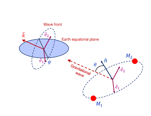
Figure 1: Two stars are orbiting each other and emit gravitational waves which are detected on Earth. Orientation of the orbital plane is described by a unit vector $\hat{n}$ perpendicular to the plane. The angle between $\hat{n}$ and the direction of the wave propagation $\hat{k}$ is the orbit inclination angle $\theta$. The wave polarization vector $\hat{e}_{1}$ is perpendicular to $\hat{k}$ and chosen to be parallel to the orbital plane, while $\hat{e}_{2}=\hat{k}\times\hat{e}_{1}$. The polarization angle $\psi$ is the angle between $\hat{e}_{1}$ and the line formed by intersection of the wave front and Earth’s equatorial plane.

We will consider a general case of a GW propagating along the unit vector $\hat{k}$; the vector $\mathbf{h}$ is perpendicular to $\hat{k}$. To be specific, we consider the generation of GWs by two compact stars with masses $M_{1}$ and $M_{2}$ moving along circular orbits with angular velocity $\Omega(t)$. We assume that the spacing between the stars is much larger than their dimensions and the motion is non-relativistic. For example, the spacing between two neutron stars of equal masses $1$ $M_{\odot}$ moving with orbital frequency $50$ Hz (i.e. the GW frequency is $100$ Hz) is $r=140$ km, which is much larger than the stellar radii $\sim 10$ km. The orbital velocity of the stars is $0.07c$. For such parameters the orbital frequency and the radius change due to emission of GWs only a little during an orbital period and one can use an adiabatic approximation. This example is relevant for the GW170817 event signal at the early inspiral stage which we analyze in this paper. At this stage, the energy loss by the binary system is described by the same quadrupole formula in vector gravity and general relativity, and, hence, both theories yield the same gravitational waveform. Such a waveform is known analytically and is accurate during almost the entire data collection time interval (apart from the last second or so before merger) for the GW170817 event involving low-mass objects.

In contrast to circular-orbit binaries, the velocity on an eccentric orbit changes over its period and the instantaneous orbital frequency also varies substantially. Orbital eccentricity leads to multiple orbital frequency harmonics in the gravitational waveform. However, since GW emission tends to circularize the orbit as it shrinks the binary separation Pete64 , many of the binary GW sources are expected to have small orbital eccentricity by the time they enter the frequency bands of ground-based GW detectors. For example, although the eccentricity of the Hulse-Taylor binary pulsar system is currently $0.6171$ Huls75 it will have an eccentricity of $\sim 10^{-4}$ when it enters the LIGO band Gond17 . Orbital eccentricity was assumed to be zero in the analysis of the detected GW sources Abbo17b ; Abbo18 and we make the same assumption in the present paper.

Neutron stars spin down due to the loss of rotational energy by powering magnetically driven plasma winds. As a consequence, the spin of neutron stars in isolated binary systems is expected to be relatively small by the time of their merger. This is consistent with the spin of neutron stars measured in the Galactic binaries (see Table III in Zhu18 ). Since no evidence for non-zero component spins was found for the binary neutron star merger GW170817 Abbo18 we will disregard effects of the neutron star spins in the present analysis.

We denote unit polarization basis vectors as $\mathbf{\hat{e}}_{1}$ and $\mathbf{\hat{e}}_{2}$. They are perpendicular to $\hat{k}$ and we choose them as shown in Fig. 1. For non-relativistic motion, using formulas of Ref. Svid17 , we obtain for vector GW in the adiabatic approximation far from the binary system

$$\mathbf{h}=A\left[\sin\theta\sin(2\phi)\mathbf{\hat{e}}_{1}+\frac{1}{2}\sin(2\theta)\cos(2\phi)\mathbf{\hat{e}}_{2}\right],$$ (3)

where

$$A=\frac{4GM\Omega^{2}r^{2}}{c^{4}R}=\frac{5^{1/4}G^{5/4}M^{5/3}}{c^{11/4}RM_{c}^{5/12}}\frac{1}{\left(t_{c}-t\right)^{1/4}}$$ (4)

is the GW amplitude which gradually increases with time due to the increase of the orbital velocity of the stars caused by emission of GWs. In Eqs. (3) and (4) $M=M_{1}M_{2}/(M_{1}+M_{2})$ is the reduced stellar mass, $r=r(t)$ is the distance between the stars,

$$\phi(t)=-\left(\frac{c^{3}}{5GM_{c}}\right)^{5/8}\left(t_{c}-t\right)^{5/8}+\phi_{0}$$ (5)

is the star azimuthal angle in the orbital plane, $t_{c}$ is the coalescence time,

$$M_{c}=\frac{\left(M_{1}M_{2}\right)^{3/5}}{(M_{1}+M_{2})^{1/5}}$$ (6)

is the chirp mass of the system, $R$ is the distance to the binary system and $\theta$ is the orbit inclination angle, that is, the angle between the normal to the orbital plane $\hat{n}$ and the direction of the wave propagation $\hat{k}$ (see Fig. 1). Depending on the inclination angle of the orbital plane of the binary stars, the GW in vector gravity can be linearly or elliptically polarized in the same way as electromagnetic waves generated by an oscillating quadrupole.

The signal of the LIGO-like interferometer with perpendicular arms of length $L_{a}$ along the direction of unit vectors $\hat{a}$ and $\hat{b}$ is proportional to the relative phase shift of the laser beam traveling a roundtrip distance $2L_{a}$ along the two arms. The relative phase shift divided by $2L_{a}\omega/c$, where $\omega$ is the angular frequency of the optical field in the interferometer, gives the gravitational wave strain $h(t)$ Svid17 ; Nish09 ; Chat12 ; Haya13 ; Pitk17 ; Alle18

$$h(t)=(\hat{a}\cdot\hat{k})(\hat{a}\cdot\mathbf{h})-(\hat{b}\cdot\hat{k})(\hat{b}\cdot\mathbf{h}).$$ (7)

Using Eqs. (3) and (7) yields the following expression for the interferometer response for the vector GW

$$h(t)=A\left(\sin\theta\sin(2\phi)V_{1}+\frac{1}{2}\sin(2\theta)\cos(2\phi)V_{2}\right),$$ (8)

where $V_{1}$ and $V_{2}$ are the detector response functions for the two basis vector polarizations $\mathbf{\hat{e}}_{1}$ and $\mathbf{\hat{e}}_{2}$

$$V_{1,2}=(\hat{a}\cdot\hat{k})(\hat{a}\cdot\mathbf{\hat{e}}_{1,2})-(\hat{b}\cdot\hat{k})(\hat{b}\cdot\mathbf{\hat{e}}_{1,2}).$$ (9)

If the same binary system emits tensor GWs according to general relativity, the metric oscillates in the $\mathbf{\hat{e}}_{1}-\mathbf{\hat{e}}_{2}$ plane as

$$h_{12}=h_{21}=A\cos\theta\sin(2\phi),$$

$$h_{11}=-h_{22}=\frac{A}{2}\left(1+\cos^{2}\theta\right)\cos(2\phi),$$

and the interferometer response is given by

$$h(t)=A\left(\frac{1}{4}\left(1+\cos^{2}\theta\right)\cos(2\phi)T_{1}+\cos\theta\sin(2\phi)T_{2}\right),$$ (10)

where $T_{1,2}$ are the interferometer response functions for the two basis tensor polarizations

$$T_{1}=(\hat{a}\cdot\mathbf{\hat{e}}_{1})^{2}-(\hat{b}\cdot\mathbf{\hat{e}}_{1})^{2}+(\hat{b}\cdot\mathbf{\hat{e}}_{2})^{2}-(\hat{a}\cdot\mathbf{\hat{e}}_{2})^{2},$$ (11)

$$T_{2}=(\hat{a}\cdot\mathbf{\hat{e}}_{1})(\hat{a}\cdot\mathbf{\hat{e}}_{2})-(\hat{b}\cdot\mathbf{\hat{e}}_{1})(\hat{b}\cdot\mathbf{\hat{e}}_{2}),$$ (12)

and $A(t)$, $\phi(t)$ are given by the same Eqs. (4) and (5) as for vector gravity.

Equations (8) and (10) show that vector GWs emitted parallel to the orbital plane ($\theta=90^{0}$) will produce the same maximum detector response as the general relativistic GWs emitted in the direction perpendicular to the plane ($\theta=0^{0},$ $180^{0}$).

Next we introduce an integrated complex interferometer response

$$I(t)=\int_{t_{0}}^{t_{0}+t}\left(t_{c}-\tau\right)^{1/4}e^{-2i\phi(\tau)}h(\tau)d\tau,$$ (13)

where $t$ is the signal collection time and $h(t)$ is the strain measured by the interferometer that contains both signal and noise. According to Eqs. (4), (8) and (10), the signal contribution to $I(t)$ is proportional to $t$ provided we disregard small correction produced by the fast oscillating term. Thus, signal accumulates with an increase of the collection time $t$. In contrast, noise does not accumulate with $t$ and for large enough $t$ the noise contribution to $I(t)$ can be disregarded. In this case for vector gravity we obtain

$$I_{V}(t)=\alpha\left(-i\sin(\theta)V_{1}+\frac{1}{2}\sin(2\theta)V_{2}\right)t,$$ (14)

while for general relativity

$$I_{T}(t)=\alpha\left(\frac{1}{4}\left(1+\cos^{2}\theta\right)T_{1}-i\cos(\theta)T_{2}\right)t,$$ (15)

where

$$\alpha=\frac{5^{1/4}G^{5/4}M^{5/3}}{2c^{11/4}RM_{c}^{5/12}}$$ (16)

is independent of time and the orientation of the interferometer arms.

Equations (14) and (15) are predictions of vector gravity and general relativity which are valid with high accuracy if the orbital frequency and radius slowly change during an orbital period. Equations (14) and (15) show that the amplitude of $I(t)$ grows linearly with the collection time $t$ and the phase of $I(t)$ is independent of $t$. Both the phase and the amplitude of $I(t)$ depend on the interferometer orientation for the vector and tensor polarizations in a fixed way. This paper tests this dependence. A verified discrepancy between observations and the predictions of a theory rules out the theory.

According to Eqs. (14) and (15), the ratio of the accumulated signals $I(t)$ measured by two interferometers, e.g. LIGO-Hanford and LIGO-Livingston, is a complex number. We denote this ratio as $H/L$. Vector gravity predicts that

$$\frac{H}{L}=\frac{2\sin(\theta)V_{H1}+i\sin(2\theta)V_{H2}}{2\sin(\theta)V_{L1}+i\sin(2\theta)V_{L2}},$$ (17)

while for the tensor polarization of general relativity

$$\frac{H}{L}=\frac{\left(1+\cos^{2}\theta\right)T_{H1}-4i\cos(\theta)T_{H2}}{\left(1+\cos^{2}\theta\right)T_{L1}-4i\cos(\theta)T_{L2}}.$$ (18)

The complex ratio $H/L$ depends on the wave polarization (tensor or vector), the direction of the wave propagation $\hat{k}$, the orientation of the interferometer arms, the orbit inclination angle $\theta$ and the polarization orientation angle $\psi$ defined in Fig. 1.

Taking the Fourier transform of Eqs. (8) and (10), we obtain the interferometer signal in the frequency representation

$$h_{V}(f)=B(f)\left[-i\sin(\theta)V_{1}+\frac{1}{2}\sin(2\theta)V_{2}\right]$$ (19)

for vector gravity, and

$$h_{T}(f)=B(f)\left[\frac{1}{4}\left(1+\cos^{2}\theta\right)T_{1}-i\cos(\theta)T_{2}\right]$$ (20)

for general relativity. Thus, in the frequency representation the ratio of signals $h(f)$ measured by two interferometers is also given by Eqs. (17) and (18). The Fourier representation can be used to check the correctness of the signal ratios obtained by the signal accumulation approach.

For the LIGO-Virgo network, the orientation of the interferometer arms and interferometer positions are accurately known LV16 . If an optical counterpart of the GW source is found then the propagation direction of GW is also accurately known. In this case the orbit inclination angle $\theta$ and polarization angle $\psi$ are the only free parameters in the signal ratios.

The three interferometers of the LIGO-Virgo network yield two independent complex ratios $H/L$ and $V/L$. In an ideal case of strong signals these two complex numbers can be accurately measured and compared with the values predicted by general relativity and vector gravity. The two measured complex numbers $H/L$ and $V/L$ depend on two real variables $\theta$ and $\psi$. Such a system of four equations with two unknowns is overdetermined and in the general case can have a solution only for tensor or vector GWs, but not for both. Thus, GW signals detected by a network of three interferometers can, in principle, decide between tensor polarization (general relativity) and vector polarization (vector gravity).

In the literature it is often mentioned that the arms of the two LIGO interferometers (Livingston and Hanford) are almost co-aligned, and hence, the ratio $H/L$ cannot give any information on the GW polarization. In fact, the angles between the corresponding arms of the two LIGO interferometers are actually not that small (taking the dot product between the arm directions yields angles $13^{\circ}$ and $24^{\circ}$ respectively, and $27^{\circ}$ between the normals to the detector planes) and hence the $H/L$ ratio can impose significant constraints on the GW polarization detected by the LIGO-Virgo network Hilb18 .

The LIGO-Virgo detection of the GW170814 event Abbo17a , attributed to binary black holes, presented the first possibility of testing the polarization properties of GWs. However, for that event, there were no concurrent electromagnetic observations, so the source location precision, although much better than the previous two-observatory detections, was not sufficient to decide between tensor and vector polarizations Max18 ; Hilb18 . The full parameter estimate of Ref. Abbo17a constrained the position of the GW source to a $90\%$ credible area of $60$ deg². It has been shown that vector GW polarization is compatible with the GW170814 event in a considerable part of the $90\%$ credible area Hilb18 . As shown explicitly in Ref. Hilb18 , the uncertainty in the GW170814 sky source location does not permit drawing definite conclusions about the GW polarization. The same would be true for GW170817 (as confirmed in Ref. Max18 , p. 12) absent the precise location information from the concurrent detection of electromagnetic emissions.

On 17 August 2017, the Advanced LIGO and Virgo detectors observed the gravitational wave event GW170817 - a strong signal from the merger of a binary neutron-star system Abbo17b . For the GW170817 event the propagation direction of the GW is accurately known from the precise coordinates of the optical counterpart discovered in close proximity to the galaxy NGC 4993. Namely, at the moment of detection the source was located at the latitude 23.37^∘ S and longitude 40.8^∘ E.

It turns out that for this source location we can distinguish between the predictions of general relativity and vector gravity even if the ratios $H/L$ and $V/L$ are obtained with relatively poor accuracy. In the next section we extract those ratios from the GW strain data released by the LIGO-Virgo collaboration LV17 . In Section III we test vector gravity and general relativity based on the obtained ratios. In Section IV we explain why polarization analysis of GW170817 by the LIGO-Virgo collaboration failed to find inconsistency with general relativity.

II GW170817 event: Data processing and signal extraction

As we have shown in the previous section, the crucial quantities for our analysis are the complex amplitude ratios $H/L$ and $V/L$. Here we use published strain time series for the three detectors LV17 . These data are not normalized to the detector’s noise (“whitened”) and, thus, can be directly used to estimate the GW signal ratios $H/L$ and $V/L$.

We bandpassed the time series data between $40$ Hz and $250$ Hz to eliminate low and high frequency noise, which improves signal processing. A short instrumental noise transient appeared in the LIGO-Livingston detector $1.1$ s before the coalescence time of GW170817. We restrict our analysis to the prior time in order to avoid this “glitch”.

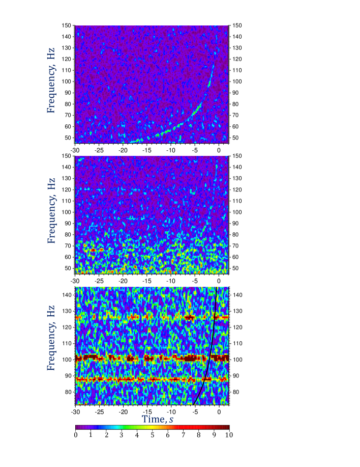
Figure 2: Spectrograms (time-frequency representations) of strain data containing the gravitational-wave event GW170817, observed by the LIGO-Livingston (top), LIGO-Hanford (middle), and Virgo (bottom) detectors. As in Ref. Abbo17b , times are shown relative to August 17, 2017 12:41:04 UTC. The amplitude scale in each spectrogram is the same. The expected position of the Virgo signal is indicated as a black solid line in the Virgo spectrogram.

Using the GW170817 source location information Abbo17b we calculated the arrival time delays of the GWs at the interferometer locations. We find that the GW arrived at the Virgo detector $0.02187$ s earlier than at the LIGO-Livingston location, and $0.00333$ s later at the LIGO-Hanford detector. We adjusted the measured strain time series for these time delays.

In Fig. 2 we plot spectrograms (time-frequency representations) of strain data containing the gravitational-wave event GW170817, observed by the LIGO-Livingston (top), LIGO-Hanford (middle), and Virgo (bottom) detectors. As in Ref. Abbo17b , times are shown relative to August 17, 2017 12:41:04 UTC. The amplitude scale in each detector is the same. In contrast to Ref. Abbo17b , we have not normalized the data to the detector’s noise amplitude spectral density which allows us to estimate the ratios of the signal amplitudes in different detectors. The figure shows that the GW signal is visible in the LIGO-Livingston and LIGO-Hanford spectrograms only in certain frequency ranges. The Virgo signal is not visible. We indicated the expected position of the Virgo signal as a black solid line in the Virgo spectrogram.

We constrain our analysis to GW frequencies below $150$ Hz. As mentioned previously, in this range the orbital inspiral of solar mass neutron stars is accurately described by the adiabatic approximation for which both vector gravity and general relativity predict the same gravitational waveform $s(t)$. In particular, $s(t)$ can be approximated as

$$s(t)\propto\frac{1}{\left(t_{c}-t\right)^{1/4}}\cos\left[2\phi(t)\right],$$ (21)

where

$$\phi(t)=-\left(\frac{c^{3}}{5GM_{c}}\right)^{5/8}\left(t_{c}-t\right)^{5/8}+bt+\phi_{0},$$ (22)

$t_{c}$ is the coalescence time and $M_{c}$ is the chirp mass of the system given by Eq. (6). In Eq. (22) we introduced a small adjustable frequency offset $b$ in order to obtain a better fit of the signal in a broad frequency range. In Eqs. (21) and (22), $M_{c}$, $t_{c}$ and $b$ are free parameters chosen to give the maximum integrated signal (13). For the best fit we found in the detector frame $M_{c}=1.195$ $M_{\odot}$, $t_{c}=0.296$ s and $b=0.83$ rad/s. The value of $M_{c}$ we obtained is close to that reported in Refs. Abbo17b ; Abbo18 .

In Figs. 3, 4 and 5 we plot the absolute value of the integrated interferometer response $|I|$ (given by Eq. (13)) as a function of the coalescence time $t_{c}$ for the three interferometers. The plots have a pronounced peak when $t_{c}=0.296$ s for LIGO-Livingston and LIGO-Hanford detectors. Thus, for these detectors the signal can be found with a high accuracy. For the Virgo detector the integrated signal is barely visible on top of the noise background (see Fig. 5).

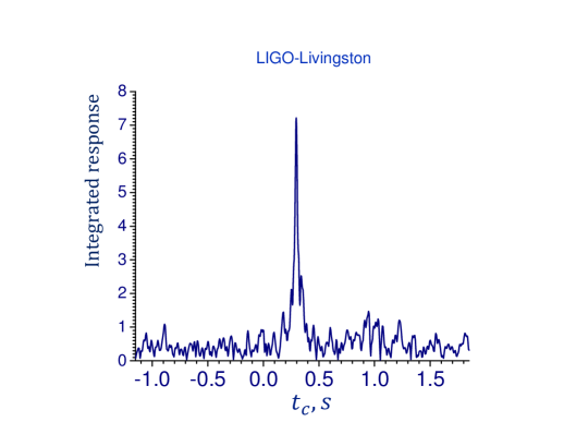
Figure 3: Absolute value of the integrated interferometer response (13) (in arbitrary units) as a function of the coalescence time $t_{c}$ for the LIGO-Livingston detector accumulated from the frequency interval $51-115$ Hz. The response is calculated using the best fit signal phase $\phi(t)$ given by Eq. (22) with $M_{c}=1.195$ $M_{\odot}$ and $b=0.83$ rad/s.

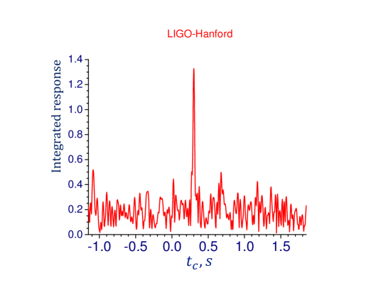
Figure 4: Absolute value of the integrated interferometer response (13) (in arbitrary units) as a function of the coalescence time $t_{c}$ for the LIGO-Hanford detector accumulated from the frequency interval $85-145$ Hz. The response is calculated using the best fit signal phase $\phi(t)$ given by Eq. (22) with $M_{c}=1.195$ $M_{\odot}$ and $b=0.83$ rad/s.

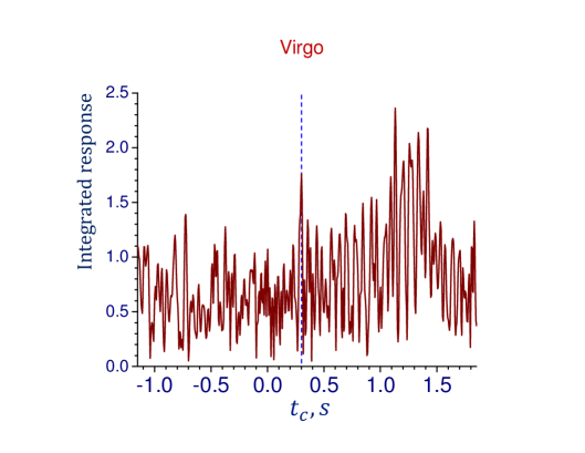
Figure 5: Absolute value of the integrated interferometer response (13) (in arbitrary units) as a function of the coalescence time $t_{c}$ for the Virgo detector accumulated from the frequency interval $73-145$ Hz. The response is calculated using the best fit signal phase $\phi(t)$ given by Eq. (22) with $M_{c}=1.195$ $M_{\odot}$ and $b=0.83$ rad/s. The vertical dashed line marks the expected position of the signal peak.

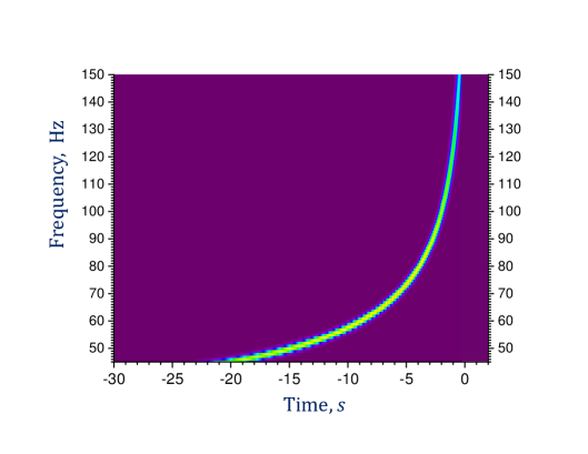
Figure 6: Spectrogram of the best fit gravitational waveform given by Eqs. (21) and (22) with $M_{c}=1.195$ $M_{\odot}$, $t_{c}=0.296$ s and $b=0.83$ rad/s. Color coding is the same as in Fig. 2.

In Fig. 6 we plot a spectrogram of the best fit gravitational waveform given by Eqs. (21) and (22). In the time-frequency representation such an idealized signal is a smooth line. In contrast, the LIGO-Livingston signal contains gaps in the spectrogram at certain frequencies (see Fig. 2 (top) and Fig. 1 in Ref. Abbo17b ). Presumably, these “gaps” are due to real-time noise filtering through various feedback loops and off-line noise subtraction applied to the LIGO-Livingston detector Abbo17b ; Abbo18 . Such a procedure eliminates noise at certain frequencies and, as one can see from the spectrogram, it also reduces the LIGO-Livingston signal at these frequencies. As a consequence, only frequency ranges for which the signal is clearly visible in the spectrogram should be used for the estimate of the LIGO-Livingston signal amplitude (for details see Section IV). We emphasize that the $H/L$ and $V/L$ ratios should be the same throughout the early inspiral stage. We accumulate the LIGO-Livingston signal from the following “good” frequency intervals

$$L:\quad 51\div 57,\quad 71\div 80,\quad 95\div 115\,\text{ Hz.}$$ (23)

This means that when we calculate the integrated interferometer response (13) we integrate only over the time intervals for which the signal passes through the frequency bands (23). This yields a total collection time of about $6$ s. The result for $|I(t)|$ as a function of the collection time $t_{\text{coll}}$ is shown in Fig. 7 (upper curve). The figure shows that the absolute value of the integrated LIGO-Livingston signal $|I(t)|$ approximately follows a straight line, in agreement with Eqs. (14) and (15).

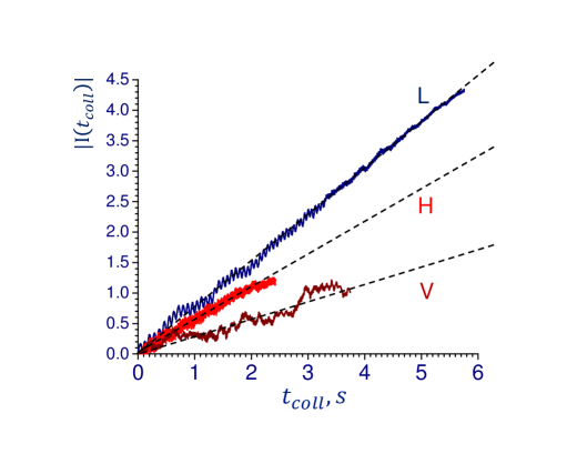
Figure 7: Absolute value of the integrated signal (13) as a function of the collection time $t_{\text{coll}}$ for LIGO-Livingston (upper curve), LIGO-Hanford (middle curve) and Virgo (bottom curve) detectors. The scale of the vertical axis is arbitrary but the same for all three detectors. The signals are collected from the frequency intervals (23), (24) and (25) respectively. The least-squares fits to the data are shown as dashed lines.

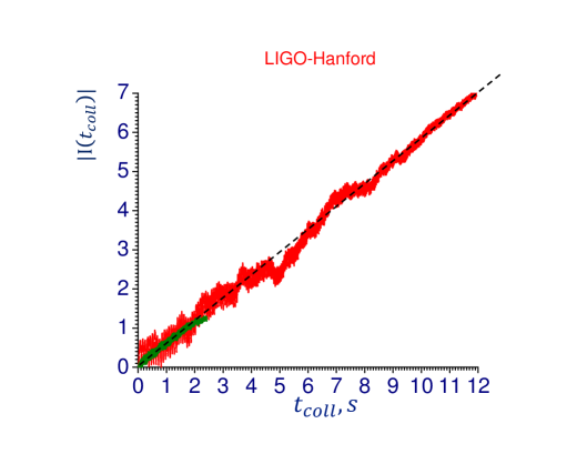
Figure 8: Absolute value of the integrated signal (13) as a function of the collection time $t_{\text{coll}}$ for the LIGO-Hanford detector collected from the frequency intervals (24) (green curve) and $51\div 115\,$ Hz (red curve). The fit to the data is shown as a dashed line.

As we show later in Section IV, the noise filtering has not appreciably affected the LIGO-Hanford signal and hence, in principle, one can use a broad frequency range for the LIGO-Hanford signal collection. However, in our estimate we collect the signal only from frequency intervals with lower noise. Namely, we choose

$$H:\quad 85\div 121,\quad 128\div 145\,\text{ Hz.}$$ (24)

This yields a collection time of about $2.5$ s. The result for the LIGO-Hanford integrated signal $|I(t)|$ is shown as the middle curve in Fig. 7, which also follows a straight line. As a check, in Fig. 8 we show that the LIGO-Hanford signal collection from a broad frequency range of $51\div 115\,$ Hz (collection time $12$ s) yields the same average slope of $|I(t)|$. Thus, the Hanford results obtained using different frequency intervals are consistent with each other.

Due to the larger amplitude noise in the Virgo observatory, the GW signal is not visible in the Virgo spectrogram. To estimate the Virgo signal we integrate the measured strain over the frequency ranges corresponding to the lowest detector noise at the expected time of the signal arrival. Namely, we accumulate signal from the following frequency intervals

$$V:\quad 73\div 85,\quad 89\div 122,\quad 130\div 145\,\text{ Hz}$$ (25)

The result is shown as the bottom curve in Fig. 7. The curve does not follow a straight line and, hence, we cannot estimate the Virgo signal with a good accuracy. However, the plot allows us to place a reliable upper limit on the Virgo signal amplitude.

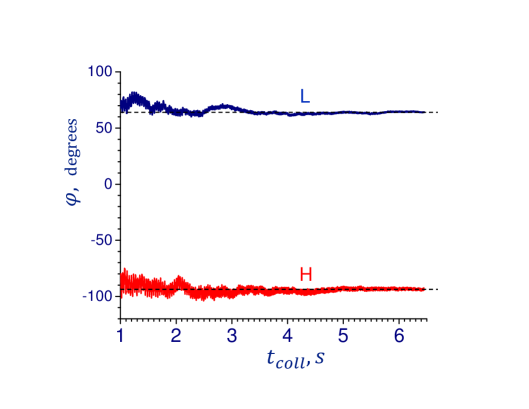
Figure 9: Phase of the integrated signal (13) as a function of the collection time for the LIGO-Livingston (upper curve) and LIGO-Hanford (lower curve) strain data. The signals are collected from the frequency range of $62\div 115\,$ Hz for both detectors. Dashed lines show the best fit phase values. Since we adjusted the measured strain time series for the arrival time delays, they do not contribute to the phase differences.

In Fig. 9 we plot the phase of the integrated signal $I(t)$ as a function of the collection time for the LIGO-Livingston and LIGO-Hanford strain data. Contrary to the amplitude, the phase of the accumulated signal is not affected if the signal is reduced at certain frequencies by the noise filtering. For the phase estimate we collected the interferometer signals in the same frequency range of $62\div 115\,$ Hz (total collection time is $6.5$ s) for both detectors. As expected, the accumulated phase is approximately constant as a function of the collection time and can be obtained with a good accuracy from the plots of Fig. 9.

Figures 7 and 9 yield the following estimates

$$\left|\frac{H}{L}\right|=0.65\pm 0.15,$$ (26)

$$\varphi_{L}-\varphi_{H}=160^{\circ}\pm 15^{\circ},$$ (27)

$$\left|\frac{V}{L}\right|<0.45,$$ (28)

where the uncertainties correspond to $2\sigma$ confidence interval ($95\%$ confidence level). The uncertainties have been calculated by injecting a test signal into the measured strain time series.

According to Eqs. (19) and (20), one can check the consistency of our estimates by calculating the ratio of the Fourier transforms of the signals in different detectors. In order to obtain the signal in the time-frequency representation we calculate the short-time Fourier transform of the measured time series $h(t)$. To do so, we divide time into intervals of length $\Delta t=0.3$ s. This is an optimal value of $\Delta t$; it covers a large enough number of GW oscillations and yet it is short enough not to wash out the signal. We calculate the Fourier transform for each time interval $[t,t+\Delta t]$

$$F(f,t)=\sum\limits_{t<t_{k}<t+\Delta t}h(t_{k})e^{-2\pi ift_{k}}$$ (29)

and plot $F(f,t)$ at fixed frequency $f$ as a function of time by changing $t$ in steps much shorter than $\Delta t$.

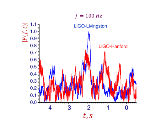
Figure 10: Absolute value of the Fourier transform of the strain $|F(f,t)|$ for the GW170817 event measured by the LIGO-Hanford (red line) and LIGO-Livingston (blue line) interferometers as a function of time at frequency $f=100$ Hz. The vertical axis is normalized such that the LIGO-Livingston GW signal amplitude is equal to $1$.

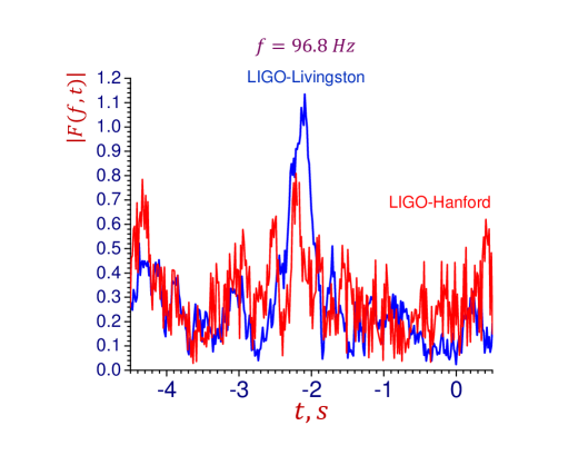
Figure 11: Absolute value of the Fourier transform of the strain $|F(f,t)|$ for the GW170817 event measured by the LIGO-Hanford (red line) and LIGO-Livingston (blue line) interferometers as a function of time at frequency $f=96.8$ Hz. The scale of the vertical axis is the same as in Fig. 10.

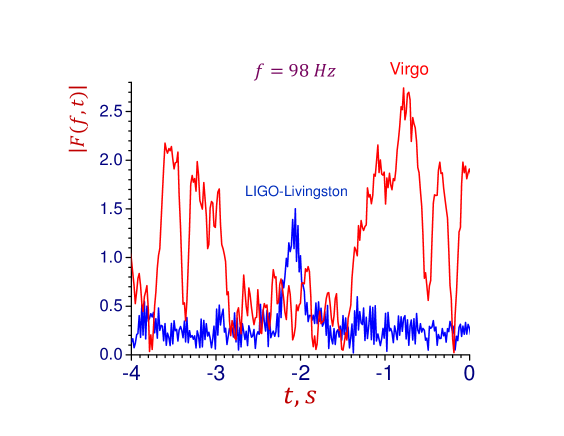
Figure 12: Absolute value of the Fourier transform of the strain $|F(f,t)|$ measured by the Virgo (red line) and LIGO-Livingston (blue line) interferometers as a function of time at frequency $f=98$ Hz. The scale of the vertical axis is the same as in Fig. 10.

The GW signal is clearly visible in the LIGO-Livingston data only over a few frequency ranges. Among them we select frequencies for which the noise of the LIGO-Hanford detector is relatively small. In Fig. 10 we plot the absolute value of the Fourier transform of the strain $|F(f,t)|$ measured by the LIGO-Livingston (blue curve) and the LIGO-Hanford (red curve) interferometers as a function of time at frequency $f=100$ Hz. The GW signal is clearly visible at $t_{0}\approx-2$ s. The vertical axis in the figure is normalized such that the LIGO-Livingston signal amplitude is equal to $1$.

Fig. 10 shows that $|H/L|$ is consistent with the estimate (26). We found that similar plots for other frequencies at which the LIGO-Livingston signal is clearly visible and the LIGO-Hanford noise level is low give the same answer. For example, Fig. 11 shows the absolute value of the Fourier transform of the strain $|F(f,t)|$ measured by the LIGO-Hanford and LIGO-Livingston interferometers as a function of time at frequency $f=96.8$ Hz. The plots shown in Fig. 11 are consistent with Eq. (26).

For the Virgo detector the noise is very high, which makes extraction of the Virgo signal a challenging task. Using Virgo data we calculated $F(f,t)$ at various frequencies $f$ and luckily found one which can be used for the signal estimate. We found that for $f=98$ Hz the Virgo noise happened to be quite low in the vicinity of the time at which the signal is expected to arrive (see Fig 12). As a result, using $F(f,t)$ for $f=98$ Hz we can constrain the $V/L$ ratio with a reasonable accuracy which yields an estimate consistent with Eq. (28).

III Test of gravitational theories

According to Eqs. (17) and (18), the complex ratios of the GW signals detected by the different interferometers depend on whether the GW is described by vector gravity or general relativity. The right hand sides of Eqs. (17) and (18) contain only two unknown parameters, the inclination and polarization angles $\theta$ and $\psi$.

According to the results of the previous section, the experimental constraints on the complex ratios $H/L$ and $V/L$ are given by Eqs. (26), (27) and (28) respectively. If there are angles $\theta$ and $\psi$ for which Eq. (17) and the corresponding equation for $V/L$ yield the measured ratios, then vector gravity agrees with the observations. Otherwise, the theory is ruled out. Eq. (18) and the corresponding equation for $V/L$ can be used to test general relativity. As mentioned previously, only one of the two theories is expected to pass this test.

III.1 Test of vector gravity

We found that for vector gravity there is a range of inclination $\theta$ and polarization $\psi$ angles compatible with the constraints (26), (27) and (28). This range is shown in Fig. 13 as the red filled area. Thus, vector gravity is compatible with the observations.

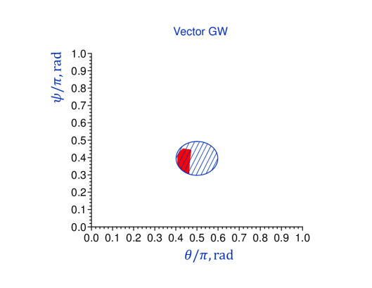
Figure 13: The region of inclination $\theta$ and polarization $\psi$ angles compatible with constraints (26), (27) and (28) for the GW170817 event assuming vector GW (red filled area). The dashed area is the region of angles calculated in the vector theory of gravity which gives a distance to the source compatible with the astronomical observations. The allowed inclination angle range is $71^{\circ}<\theta<84^{\circ}$.

Next we show that vector gravity also gives the correct distance to the source. Eq. (3) tells us that in vector gravity the intensity of GWs emitted at the inclination angle $\theta$ is proportional to

$$I_{VG}\propto\sin^{2}\theta\left(1+\cos^{2}\theta\right),$$ (30)

that is, the GW emission is maximum in the orbital plane ($\theta=\pi/2$) and is equal to zero perpendicular to the plane ($\theta=0,$ $\pi$). On the other hand, for general relativity we have Land95

$$I_{GR}\propto 4\cos^{2}\theta+(1+\cos^{2}\theta)^{2}.$$ (31)

The emission intensity peaks in the direction perpendicular to the orbital plane ($\theta=0,$ $\pi$) and drops by a factor of eight for the in-plane emission.

NGC 4993 located at a distance $43.8_{-6.9}^{+2.9}$ Mpc was identified as the host galaxy of GW170817 Abbo17b . It has been shown that a general relativistic GW yields the right distance to the source at the $95.4\%$ ($2\sigma$) credible level if $|\cos\theta|>0.75$ Abbo17c . Using Eqs. (19) and (20) we calculated the region of $\theta$ and $\psi$ angles for which the amplitude of the $L$ signal in vector gravity is equal to that produced by a general relativistic GW coming from the same binary system with $|\cos\theta|>0.75$. Direct calculations based on Eqs. (3) and (4), known parameters of the binary system Abbo18 and the amplitude of the $L$ signal yield similar results.

The constraints on $\theta$ and $\psi$ obtained in vector gravity based on the known distance to the source are shown in Fig. 13 as the dashed area. The dashed and filled red regions have considerable overlap. Thus, vector gravity yields a distance to the source compatible with the astronomical observations, but with a different conclusion about the binary orbit’s inclination angle.

One should note that Fig. 13 constrains the orbit inclination angle $\theta$ to the range $71^{\circ}<\theta<84^{\circ}$, that is, according to vector gravity, the line-of-sight is close to the orbital plane of the inspiraling stars. This suggests that the faint short gamma-ray burst detected $1.7$ s after GW170817 was not produced by a canonical relativistic jet viewed at a small angle. The canonical jet scenario is also in tension with the peak energy of the observed gamma-ray spectrum Ioka19 . The detected gamma-ray burst probably was produced by a different mechanism, e.g. by elastic scattering of the jet radiation by a cocoon Kisa15 ; Kisa17 ; Kisa18 or by a shock breakout of the cocoon from the merger’s ejecta Kasl17 ; Gott18 ; Naka18 ; Ioka19a .

Later observations with VLBI discovered a compact radio source associated with the GW170817 remnant exhibiting superluminal apparent motion between two epochs at $75$ and $230$ days post-merger Mool18 . This indicates the presence of energetic and narrowly collimated ejecta observed from an angle of about $20$ degrees at the late-time emission Mool18 . Typically ejecta of spinning neutron stars consist of polar jets directed along the pulsar spin-axis and a much brighter equatorial wind. Since vector gravity constrains the line-of-sight close to the orbital plane the observed compact superluminal source is probably associated with the stellar equatorial wind.

III.2 Test of general relativity

We found that for a general relativistic tensor GW there are no combinations of inclination $\theta$ and polarization $\psi$ angles compatible with constraints (26), (27) and (28) (see Fig. 14). Uncertainties in Eqs. (26), (27) and (28) correspond to $2\sigma$ confidence interval. We found that general relativity is incompatible with constraints (26), (27) and (28) if the uncertainties are increased upto $2.5\sigma$. Therefore, the general theory of relativity is inconsistent with the data at the $2.5\sigma$ ($99\%$ confidence) level.

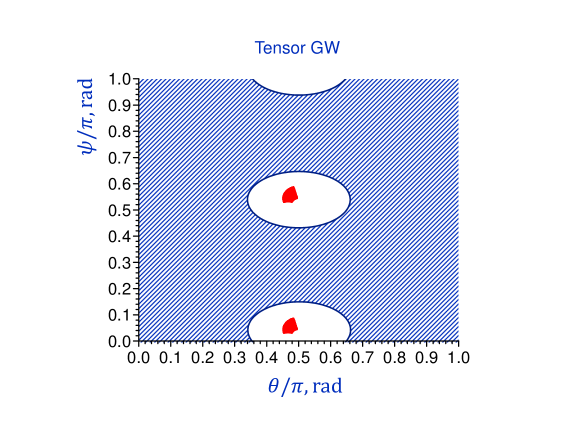
Figure 14: The range of inclination $\theta$ and polarization $\psi$ angles for general relativistic GWs compatible with constraints (26), (27) (red filled region) and (28) (blue shaded region). The red and blue regions do not overlap. Thus, there is no range of $\theta$ and $\psi$ compatible with constraints (26), (27) and (28) simultaneously.

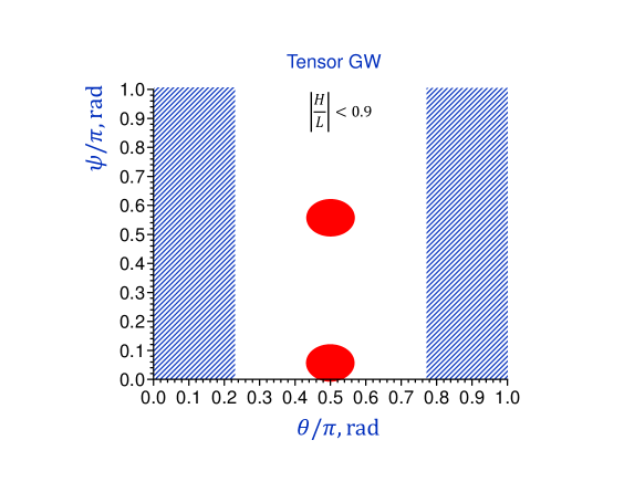
Figure 15: The region of inclination $\theta$ and polarization $\psi$ angles compatible with the single constraint $|H/L|<0.9$ for the GW170817 event assuming general relativistic GWs (red filled ovals). No constraint on $V/L$ was imposed. The blue shaded rectangles show the region of inclination angles which give a distance to the source compatible with the astronomical observations.

A skeptical reader might argue that constraints (26), (27) and (28) are too restrictive or the procedure we used is not accurate. Anticipating such criticism, we next show that general relativity is at odds with observations even if we estimate the $|H/L|$ ratio directly from the Fourier transform of the gravitational-wave strain data without using the signal accumulation algorithm. Plots of the Fourier transform in Figs. 10 and 11 show that at least $|H/L|<0.9$. Note that the short-time Fourier transform method complements the signal accumulation method because it is independent of the details of the waveform model.

It turns out that general relativity can be ruled out even based on the single constraint $|H/L|<0.9$. In Fig. 15 we plot the region of inclination $\theta$ and polarization $\psi$ angles compatible with the GW170817 event assuming general relativistic GWs and $|H/L|<0.9$ (red filled ovals). No constraint on $V/L$ was imposed. The blue shaded rectangle regions indicate inclination angles which yield a distance to the source compatible with the astronomical observations at the $2\sigma$ level ($|\cos\theta|>0.75$ Abbo17c ). Since the blue and red regions do not overlap, we conclude that general relativistic GW can not simultaneously give the right distance to the source and be compatible with the measured ratio $|H/L|$.

The constraint on the ratio $|H/L|$ is crucial for distinguishing between general relativity and vector gravity. Usually the importance of this constraint is not appreciated due to common belief that the two LIGO instruments are nearly co-aligned and, thus, $|H/L|$ can not give additional constraint on the GW polarization Isi17 . As we mentioned in the Introduction, the angles between the corresponding arms of the two LIGO interferometers are actually not that small ($13^{\circ}$ and $24^{\circ}$ respectively) and hence the $H/L$ ratio can impose significant constraints.

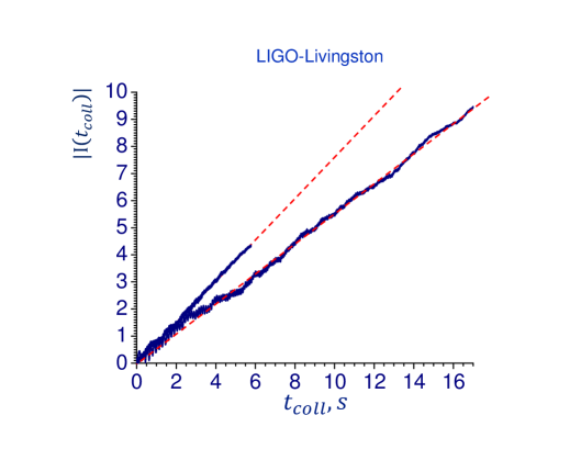
Figure 16: Absolute value of the integrated signal (13) as a function of the collection time $t_{\text{coll}}$ for the LIGO-Livingston detector collected from the “good” frequency intervals (23) (upper curve) and from a wide frequency range $45\div 115\,$ Hz (lower curve). The best fit curves are shown as dashed lines.

We want to emphasize that in order to avoid a systematic error in determining the LIGO-Livingston signal amplitude one should accumulate the signal only from the frequency intervals for which the signal is clearly visible in the spectrogram. This eliminates contributions from the regions at which signal was reduced by noise filtering. Not doing so can result in a substantial underestimate of the LIGO-Livingston signal amplitude as demonstrated in Fig. 16. The figure shows that the integrated signal $|I(t)|$ collected from a wide frequency range $45\div 115$ Hz does not follow a straight line and yields substantially smaller average slope of the $|I(t)|$ curve (the average signal per unit collection time).

An underestimate of the LIGO-Livingston signal increases the $|H/L|$ ratio which can mimic agreement with general relativity. We believe that such an underestimation error has been made in the LIGO-Virgo polarization analysis of GW170817 Max18 which we discuss next.

IV Comment on LIGO-Virgo polarization analysis of GW170817

In a recent paper Max18 the LIGO-Virgo collaboration reported results of the GW polarization test with GW170817 performed using a Bayesian analysis of the signal properties with the three LIGO-Virgo interferometer outputs. The authors found overwhelming evidence in favor of pure tensor polarization over pure vector with an exponentially large Bayes factor. This result is opposite to our present findings. Here we explain why we came to the opposite conclusion and argue that the results reported in Max18 should be reconsidered by removing the depleted frequency intervals from the LIGO-Livingston strain time series.

According to Eqs. (14) and (15) the integrated interferometer response $I(t)$ grows linearly with the collection time $t$ and the phase of $I(t)$ is independent of $t$. Thus, the theory predicts that the ratio

$$u=\frac{I(t)}{t}$$ (32)

should be independent of the signal collection time interval $[t_{0},t_{0}+t]$. This ratio can be interpreted as a signal per unit time. $u$ can be used to determine how much signal is present in the interferometer data stream at different times. If noise filtering has not altered the signal at certain frequencies then $u$ should have the same (complex) value for any collection time interval.

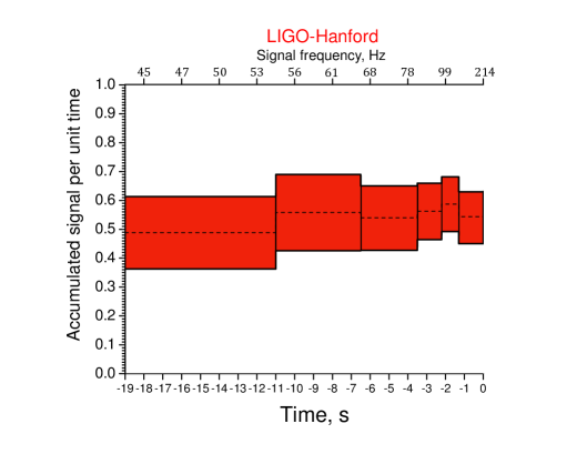
Figure 17: Absolute value of the signal per unit time $|u|$ measured by LIGO-Hanford detector for the GW170817 event for different collection time intervals. As in Ref. Abbo17b , times are shown relative to August 17, 2017 12:41:04 UTC.

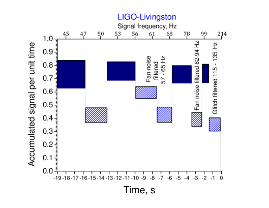
Figure 18: The same as in Fig. 17, but for the LIGO-Livingston detector. The scale of the vertical axis is arbitrary but the same in both figures. Frequency regions in which the signal is reduced by noise filtering are indicated as dashed bars.

In Fig. 17 we plot $|u|$ for LIGO-Hanford detector for different collection time intervals. The result is shown as a set of rectangular bars. The length of a bar is equal to the collection time $t$, while the height corresponds to the uncertainty produced by the detector noise. Namely, the half-height is equal to one standard deviation. We calculated the uncertainty by injecting a test signal into the measured strain time series before and after the GW170817 event. The average value of $|u|$ for each interval $t$ is indicated by a dashed line. The figure shows that $|u|$ for the LIGO-Hanford detector is consistent with a constant for the entire time when the signal is present in the data stream. Therefore, the signal in the LIGO-Hanford strain time series appears not to be affected by the noise mitigation.

In Fig. 18 we plot $|u|$ for LIGO-Livingston detector. The uncertainty bars for this detector are somewhat smaller due to lower noise. Solid color bars indicate regions for which signal is clearly visible in the LIGO-Livingston spectrogram (see Fig. 2 top panel). The vertical position of the solid color bars is consistent with $u$ being a constant, as predicted by the theory. Dashed bars correspond to gap regions in the spectrogram. Fig. 18 shows that the signal in these regions is substantially smaller than the signal content in other intervals.

The signal reduction can be attributed to noise removal which is partially performed in real time using various feedback loops. “Before noise subtraction” strain data published by the LIGO-Virgo collaboration LV17 already went through the real-time noise removal which mainly involves filtering of mechanical noise. In the “after noise subtraction” data some additional noise contributions have been eliminated. Namely, the off-line noise subtraction removed 60 Hz AC power mains harmonics from the LIGO-Livingston data stream and a glitch which occurred in the detector about $1.1$ s before coalescence. The latter can explain why there is less signal in the data stream during the glitch duration. Namely, the off-line glitch removal from the data stream led to a reduction of the GW signal in that time segment, as one can see from Fig. 18. The signal reduction in other frequency regions of the LIGO-Livingston detector can be attributed to real-time filtering of fan noise (see Fig. 3 in Cost18 ).

Usually it is believed that noise filtering does not reduce the signal substantially. But this is just an assumption which must be tested in an experiment with real gravitational waves. Because GW170817 involves orbital inspiral of low-mass stars the GW signal slowly passes through the detector frequency band. This allows us to determine the amount by which GW signal is suppressed by the noise removal at different frequencies. It seems possible that the noise filtering yields substantial signal reduction at certain frequencies for GW events for which the GW signal per unit time is very weak, which is the case for GW170817. Thus, for such events one should perform a consistency check of Figs. 17 and 18, and remove “corrupted” frequency intervals from the data analysis. This must be taken into account in the analysis of future GW events produced by inspiral of low-mass objects.

Contrary to the amplitude situation, we found that the signal phase was not altered in the Livingston and Hanford detectors, namely the phase of $u$ is consistent with a constant (see Fig. 9). Source triangulation maybe obtained using differences in arrival times of the signal in various detectors Fair18 . For the GW170817 event the Hanford-Livingston delay can be found with a high accuracy by fitting the signal phase $\phi(t)$ for hundreds of GW cycles. Since the signal phase was not altered by noise filtering the source triangulation from the Hanford-Livingston delay is predicted correctly.

As we showed in the previous section, the ratio of LIGO-Hanford and LIGO-Livingston signal amplitudes $|H/L|$ is crucial for distinguishing between tensor and vector GW polarizations. In Section II we obtained this ratio by accumulating the LIGO-Livingston signal only from the regions shown by the solid color bars in Fig. 18. In these regions the signal is not depleted. We found $0.5<\left|H/L\right|<0.8$ at the $2\sigma$ confidence level. This estimate, combined with constraints (27) and (28), is compatible with the vector theory of gravity Svid17 ; Svid18 but rules out general relativity.

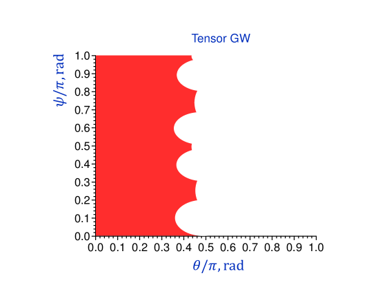
Figure 19: Range of inclination $\theta$ and polarization $\psi$ angles for general relativistic GWs compatible with constraints $1.1<|H/L|<1.3$, $\varphi_{L}-\varphi_{H}=160^{\circ}\pm 15^{\circ}$ and $|V/L|<0.77$ for the GW170817 event (red filled region).

However, signal accumulation from the entire frequency band erroneously underestimates the LIGO-Livingston signal amplitude yielding $1.1<\left|H/L\right|<1.3$ and $\left|V/L\right|<0.77$ Remark . This incorrect estimate results in the opposite conclusion about GW polarization. Namely, it rules out vector polarization, but is consistent with tensor polarization (see Fig. 19). This is what the authors of Ref. Max18 have found. The incorrect estimate of $|L|$ also explains why the sky location of the source is nevertheless predicted correctly with tensor polarization (general relativity).

One should mention that inconsistencies in the LIGO-Livingston data at different GW frequencies have been also found in the Bayesian estimation of the binary tidal deformability $\tilde{\Lambda}$ Nari18 . Namely it has been shown that the probability distribution for $\tilde{\Lambda}$ obtained from the LIGO-Livingston strain time series changes irregularly under variation of the maximum frequency of the data used in the analysis. These inconsistent features are not observed for the Hanford detector Nari18 .

We also performed polarization analysis in a Bayesian framework (that has been used by the LIGO-Virgo collaboration) taking into account the Livingston signal amplitude reduction in certain frequency regions. We found that the data give a $10^{8}$ Bayes factor favoring vector polarization over tensor.

The same method shows that if the analysis uses the smaller Livingston GW amplitude that results from including the signal depleted regions, then the Bayes factor favors tensor polarization by an exponentially large factor. That is what the LIGO-Virgo collaboration claims. The Bayesian analysis confirms that getting the relative amplitude ratios correct is absolutely critical and that if we use the “correct” amplitude ratios, the GW170817 data strongly favor vector polarization.

V Null stream analysis

Our conclusion about vector polarization of GWs can be tested using the null stream approach. This method is based on a mathematical fact that if GW has pure tensor or pure vector polarization then there exists a linear combination of the signals detected by three interferometers which gives null Gurs89 ; Wen05 ; Chat06 ; Hagi18 . The null combination depends on the GW propagation direction and orientation of the interferometer arms which are accurately known for the GW170817 event, but is independent of the unknown orientation of the orbital plane.

We calculated the null streams for the GW170817 event assuming pure tensor and pure vector polarizations. The results for the null stream combinations are

$$Null_{\text{tensor}}=0.205H+0.388L+0.407V,$$ (33)

$$Null_{\text{vector}}=0.540H+0.310L+0.150V,$$ (34)

where $H$, $L$ and $V$ are the signals in the LIGO-Hanford, LIGO-Livingston and Virgo detectors adjusted for the arrival time delays.

It is remarkable that very noisy Virgo signal enters the null stream for vector GW (34) with a much smaller weight than that for the tensor null stream. As a consequence, the vector null stream is substantially less noisy than the tensor null stream. Therefore, use of the vector null stream combination is favorable for distinguishing between pure vector and pure tensor polarizations for the GW170817 event.

In Fig. 20 we plot the spectrogram of the null stream corresponding to the vector polarization for the GW170817 event. The spectrogram is not very noisy, especially at high frequencies. No residual signal is visible in the null-vector spectrogram which supports our conclusion about vector GW polarization.

By applying the signal accumulation approach to the null stream one can obtain an upper-bound on the residual signal amplitude present in the vector null stream. In Fig. 21 we plot the absolute value of the integrated response as a function of the coalescence time $t_{c}$. The signal is accumulated from “good” frequency intervals $71-80$ Hz and $95-115$ Hz. The blue line shows the integrated response for the vector null stream

$$I_{\text{null-v}}=\left|I(0.540H+0.310L+0.150V)\right|.$$ (35)

It is at the level of noise for all $t_{c}$. The red line shows the sum of the absolute values of the integrated responses for each detector taken with the same weights as they enter the null stream

$$I_{\text{max-v}}=0.540|I(H)|+0.310|I(L)|+0.150|I(V)|.$$ (36)

The red line has a pronounced peak which yields the signal amplitude in the strain data if the detector responses are added up constructively. One can see from Fig. 21 that the amplitude of the residual signal in the vector null stream (blue line) is compatible with zero.

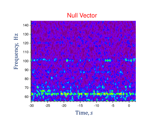
Figure 20: Spectrogram of the null stream (34) corresponding to the vector polarization for the GW170817 event. The amplitude scale in the spectrogram is the same as in Fig. 2. The red dotted line indicates the expected position of the signal.

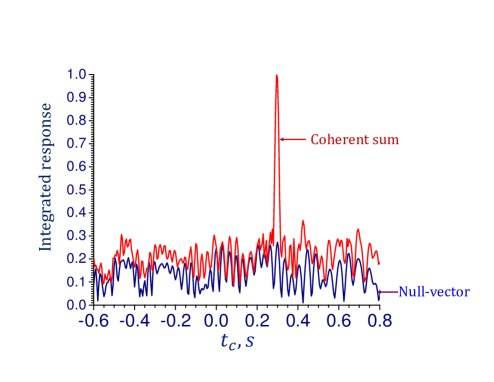
Figure 21: Absolute value of the integrated response as a function of the coalescence time $t_{c}$ for the coherent sum of the detector signals $I_{\text{max-v}}$ (red line) and the null stream for the vector GW polarization $I_{\text{null-v}}$ (blue line).

Let us now assume that GW has tensor polarization. Then residual signal should be present in the vector null stream and the ratio $I_{\text{null-v}}/I_{\text{max-v}}$ will be nonzero. The ratio depends on the inclination and polarization angles $\theta$ and $\psi$. This dependence can be calculated using Eqs. (10), (11) and (12). In Fig. 22 we plot $I_{\text{null-v}}/I_{\text{max-v}}$ as a function of $\theta$ and $\psi$ for tensor GW. The red dashed area indicates values of $\theta$ compatible with the known distance to the source ($\theta<0.23\pi$ rad or $\theta>0.77\pi$ rad Abbo17c ). The plot shows that for the range of the inclination angle compatible with the distance to the source the ratio $I_{\text{null-v}}/I_{\text{max-v}}$ exceeds $0.38$. If so, for tensor GW the residual signal should be visible in the blue curve $I_{\text{null-v}}$ of Fig. 21, which is not the case. Hence, the vector null stream combination, together with the additional constraint on $\theta$ based on the known distance to the source, rules out tensor GW polarization.

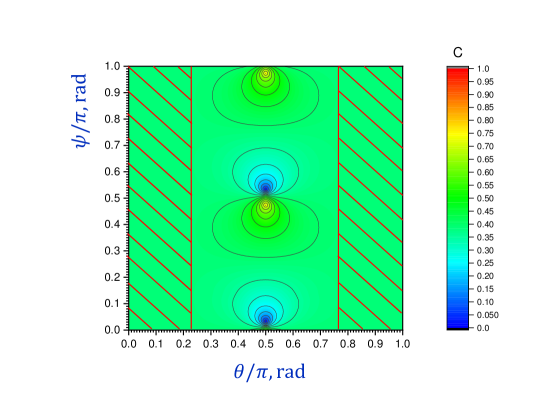
Figure 22: Ratio of the vector null stream $I_{\text{null-v}}$ to $I_{\text{max-v}}$ for tensor GW for the GW170817 event as a function of the inclination and polarization angles $\theta$ and $\psi$. Red dashed area indicates values of $\theta$ compatible with the known distance to the source.

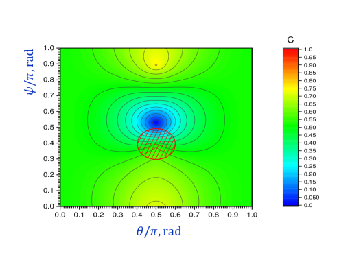
Figure 23: Ratio of the tensor null stream $I_{\text{null-t}}$ to $I_{\text{max-t}}$ for vector GW for the GW170817 event as a function of the inclination and polarization angles $\theta$ and $\psi$. Red dashed area indicates values of $\theta$ and $\psi$ compatible with the known distance to the source.

One should note that vector GW can produce a very small residual signal in the tensor null stream (33) for the GW170817 event. In Fig. 23 we plot $I_{\text{null-t}}/I_{\text{max-t}}$ as a function of $\theta$ and $\psi$ for vector GW. The plot shows that for certain values of $\theta$ and $\psi$ compatible with the known distance to the source (red dashed area in Fig. 23) the value of $I_{\text{null-t}}$ could be very small. Thus, vector GW can mimic tensor polarization in the null stream analysis of GW170817.

VI Summary and Outlook

The simultaneous detection of GWs by the three interferometers of the LIGO-Virgo network, together with the known sky location of the source, can be used to distinguish between general relativity Eins15 and vector gravity Svid17 ; Svid18 , and rule out one of the two theories. However, the possibility of coming to a decisive conclusion depends on how accurately we can find the ratios of the signals ($H/L$ and $V/L$) measured by different interferometers.

Here we have analyzed the data from GW170817 event produced by a pair of inspiraling neutron stars and observed by the LIGO-Hanford, LIGO-Livingston and Virgo interferometers. The optical counterpart of GW170817 was found which yielded accurate localization of the source in close proximity to the galaxy NGC 4993 Abbo17b .

To obtain the $H/L$ and $V/L$ ratios, we used the strain time series for the three detectors released by the LIGO-Virgo collaboration LV17 . For the GW170817 event the GW signal is clearly visible in the LIGO-Livingston and LIGO-Hanford data. However, this is not the case for the Virgo data due to larger detector noise.

We extracted the signals from the noisy data by applying the signal accumulation procedure, and then calculated $H/L$ and $V/L$ ratios and their uncertainties. We found that signal ratios are consistent with the vector theory of gravity Svid17 ; Svid18 . Also we found that vector gravity yields a distance to the source in agreement with the astronomical observations.

In contrast, we discovered that the signal ratios are inconsistent with general relativity at the $2.5\sigma$ level. Moreover, we found that general relativity is at odds with observations even if we use a much less restrictive constraint based only on the $|H/L|$ ratio obtained directly from the Fourier transform of the gravitational-wave strain data. If our analysis is correct and the detectors were properly calibrated, Einstein’s general theory of relativity is ruled out at the $99\%$ confidence level and future GW detections with three or more GW observatories should confirm this conclusion with a greater accuracy.

One should mention that BAYESTAR Sing16 and LALInference Veit15 codes commonly used for sky localization and estimation of the binary system parameters tacitly assume that signal is not corrupted by noise filtering and analyze the data from the entire detector bandwidth. In Section IV we showed that the measured LIGO-Livingston signal for GW170817 is substantially reduced at certain frequency intervals which can be attributed to noise filtering. We found that if these regions are excluded from the analysis then data are consistent with vector GW polarization and not with tensor. However, if the signal accumulation method is applied over the entire detector bandwidth, including the regions in which the signal is depleted by noise subtraction, the result underestimates the LIGO-Livingston signal amplitude. That smaller amplitude then leads to an erroneous conclusion that favors tensor polarization over vector polarization for the GW. This is what the LIGO-Virgo collaboration claims Max18 .

What are possible alternatives to general relativity? Historically in the literature, there have been many attempts at constructing different theories of gravity and most of them were ruled out Will93 ; Will14 . To the best of our knowledge, the only viable alternative theory, which also passes the present test, is the vector theory of gravity Svid17 ; Svid18 . Despite fundamental differences in the nature of the two theories, vector gravity and general relativity are equivalent in the post-Newtonian limit. The two theories also give the same quadrupole formula for the rate of energy loss by orbiting binary stars due to emission of GWs.

In strong fields, vector gravity deviates substantially from general relativity and yields no black holes. In particular, since the theory predicts no event horizons, the end point of a gravitational collapse is not a point singularity but rather a stable star with a reduced mass. We note that black holes have never been observed directly and the usually-cited evidence of their existence is based on the assumption that general relativity provides the correct description of strong field gravitation.

In vector gravity, neutron stars can have substantially larger masses than in general relativity and previous GW detection events can be interpreted in the framework of vector gravity as produced by the inspiral of two neutron stars rather than black holes Svid17 . Vector gravity predicts that the upper mass limit for a nonrotating neutron star with a realistic equation of state is of the order of $35$ M_⊙ (see Sec. $13$ in Svid17 ). Stellar rotation can increase this limit to values in the range of $50$ M_⊙. The predicted limit is consistent with masses of compact objects discovered in X-ray binaries Casa14 and those obtained from gravitational wave detections LIGO18 .

Vector gravity also predicts the existence of gaps in the neutron star mass distribution, although the position of the gaps depends on the uncertain equation of state. A $3-5M_{\odot}$ gap has been found in the low-mass part of the measured compact object mass distribution in the Galaxy Ozel10 ; Farr11 . Vector gravity predicts that neutron stars with mass above the $3-5M_{\odot}$ gap are very different from the low-mass counterpart because they belong to a different branch of the star stability region and have several orders of magnitude higher baryonic number density in their interior.

Because properties of matter at such high density are unknown, the composition of massive neutron stars is uncertain and could be very different from the low-mass counterpart. A different composition might result in a weaker emission of electromagnetic waves upon merger of these objects. This could be a reason, in addition to a large distance to the source, why optical counterparts were not discovered for GW events involving massive objects. Another possible reason is that sky localization of the GW sources was predicted incorrectly assuming tensor GW rather than vector, see e.g. Fig. 6.2 in MaxPhD for GW170814 sky location reconstructed under the assumption of different polarization hypotheses. There are however some indications that these types of GW mergers were actually followed by electromagnetic emission Conn16 ; Stal17 .

For cosmology, vector gravity gives the same evolution of the Universe as general relativity with a cosmological constant and zero spatial curvature. However, vector gravity, as mentioned in the Introduction, provides an explanation of dark energy as the energy associated with a longitudinal gravitational field induced by the expansion of the Universe and predicts, with no free parameters, the value of the cosmological constant which agrees with observations Svid17 ; Svid18 .

Vector gravity, if confirmed, can also lead to a breakthrough in the problem of dark matter. Namely, the theory predicts that compact objects with masses greater than $10^{5}M_{\odot}$ found in galactic centers have a non-baryonic origin and, thus, an as-yet-undiscovered dark matter particle is a likely ingredient of their composition. As a result, observations of such objects can allow us to ascertain the nature of dark matter.

It is interesting to note that properties of supermassive compact objects at galactic centers can be explained quantitatively in the framework of vector gravity assuming they are made of dark matter axions and the axion mass is about $0.6$ meV (see Sec. 15 in Svid17 and Ref. Svid07 ). Namely, those objects are axion bubbles. The bubble mass is concentrated in a thin interface between two degenerate vacuum states of the axion field. If the bubble radius is large, surface tension tends to contract the bubble. When the radius is small, for a bubble-like object vector gravity effectively produces a large repulsive potential which forces the bubble to expand. As a result, the bubble radius oscillates between two turning points. The radius of the $4\times 10^{6}M_{\odot}$ axion bubble at the center of the Milky Way is predicted to oscillate with a period of $20$ mins between $1$ $R_{\odot}$ and $1$ astronomical unit ($215$ $R_{\odot}$) Svid07 .

This prediction has important implications for capturing the first image of the shadow of the supermassive object at the center of the Milky Way with the Event Horizon Telescope (EHT) Godd17 . Namely, because of size oscillation the relatively low-mass bubble at the center of the Milky Way produces a shadow by bending light rays from the background sources only during short time intervals when the bubble size is smaller or of the order of the gravitational radius $r_{g}=2GM/c^{2}=17$ $R_{\odot}$. Since typical EHT image collection time is several hours, the time averaging yields a much weaker shadow than that expected from a static black hole in general relativity. In the time-averaged image, the shadow will probably be invisible.

One should mention that first image of the Milky Way center with Atacama Large Millimeter Array at $3.5$ mm wavelength has been reported recently (see Fig. 5 in Issa19 ). The resolution of the detection is only slightly greater than the size of the black hole shadow. Still, a decrease in the intensity of light toward the center should be visible. But the image gets brighter (not dimmer) closer to the center. This agrees with the predictions of vector gravity.

On the other hand, a much heavier axion bubble in the M87 galaxy ($M=4\times 10^{9}M_{\odot}$ Wals13 ) does not expand substantially during oscillations. The bubble in M87 has a mass close to the upper limit and, according to vector gravity, its radius is close to $r_{g}/4$ Svid07 . For such bubble the gravitational redshift of the bubble interior is $z=e^{2}-1\approx 6.4$. The redshift reduces radiation power coming from matter trapped inside the bubble by a factor of $(1+z)^{2}=e^{4}\approx 55$, that is the bubble interior mimics a black hole.

The large accretion disk surrounding the bubble in M87 produces radio emission which is imaged by EHT. The size of the dark hole in the disc (which has a radius of $\approx 2.6r_{g}$) is determined by the size of the innermost stable circular orbit. For massive particles, the location of the innermost stable circular orbit for the exponential metric of vector gravity in the curvature coordinates is $3.17r_{g}$ Boon19 which is close to that in Schwarzschild spacetime $3r_{g}$ Photo . As a consequence, the axion bubble in M87 produces an image similar to that of a black hole. Recent imaging of the supermassive compact object at the center of M87 with EHT at $1.3$ mm EHT19 is consistent with this expectation. Due to bubble oscillations the shadow of the M87 central object might vary on a timescale of a few days, which can be studied in the future EHT campaigns.

Presumably some dark matter bubbles harbor a fast spinning massive neutron star or a magnetar which produces relativistic jet and occasional outbursts of radiation when matter accretion accumulates critical density of hydrogen on the stellar surface to ignite runaway hydrogen fusion reactions.

This work was supported by the Air Force Office of Scientific Research (Award No. FA9550-18-1-0141), the Office of Naval Research (Award Nos. N00014-16-1-3054 and N00014-16-1-2578) and the Robert A. Welch Foundation (Award A-1261). This research has made use of data obtained from the LIGO Open Science Center (https://losc.ligo.org), a service of LIGO Laboratory, the LIGO Scientific Collaboration and the Virgo Collaboration.

References

- (1) B. P. Abbott et al. (LIGO Scientific Collaboration and Virgo Collaboration), GW170814: A Three-Detector Observation of Gravitational Waves from a Binary Black Hole Coalescence, Phys. Rev. Lett. 119, 141101 (2017).
- (2) B. P. Abbott et al. (LIGO Scientific Collaboration and Virgo Collaboration), GW170817: Observation of Gravitational Waves from a Binary Neutron Star Inspiral, Phys. Rev. Lett. 119, 161101 (2017).
- (3) A. Einstein, Die Feldgleichungen der Gravitation, Sitzungsber. Preuss. Akad. Wiss. pt. 2, 844-847 (2015).
- (4) A. A. Svidzinsky, Vector theory of gravity: Universe without black holes and solution of dark energy problem, Physica Scripta 92, 125001 (2017).
- (5) A. A. Svidzinsky, Simplified equations for gravitational field in the vector theory of gravity and new insights into dark energy, Physics of the Dark Universe 25, 100321 (2019).
- (6) D. M. Eardley, D. L. Lee, A. P. Lightman, R. V. Wagoner and C. M. Will, “Gravitational-Wave Observations as a Tool for Testing Relativistic Gravity,” Phys. Rev. Lett. 30, 884 (1973).
- (7) D. M. Eardley, D. L. Lee, A. P. Lightman, “Gravitational-Wave Observations as a Tool for Testing Relativistic Gravity,” Phys. Rev. D 8, 3308 (1973).
- (8) C. M. Will, The Confrontation between General Relativity and Experiment, Living Rev. Relativity 17, 4 (2014).
- (9) Collaboration, Planck, P.A.R. Ade, N. Aghanim, C. Armitage-Caplan et al., Planck 2013 results. XVI. Cosmological parameters, A&A 571, A16 (2014).
- (10) LIGO-Virgo Collaboration, Data release for event GW170817, Gravitational-wave strain data 16384 Hz sampling rate, https://losc.ligo.org/events/GW170817
- (11) B. P. Abbott et al. (LIGO Scientific Collaboration and Virgo Collaboration), Tests of General Relativity with GW170817, arXiv:1811.00364 [gr-qc] (2018).
- (12) A. Nishizawa, A. Taruya, K. Hayama, S. Kawamura and M. Sakagami, “Probing non-tensorial polarization of stochastic gravitational-wave backgrounds with ground-based laser interferometers,” Phys. Rev. D 79, 082002 (2009).
- (13) K. Chatziioannou, N. Yunes and N. Cornish, “Model-independent test of general relativity: An extended post-Einsteinian framework with complete polarization content,” Phys. Rev. D 86, 022004 (2012).
- (14) K. Hayama and A. Nishizawa, “Model-independent test of gravity with a network of ground-based gravitational wave detectors,” Phys. Rev. D 87, 062003 (2013).
- (15) M. Isi, M. Pitkin and A. J. Weinstein, “Probing dynamical gravity with the polarization of continuous gravitational waves,” Phys. Rev. D 96, 042001 (2017).
- (16) B. Allen, “Can a pure vector gravitational wave mimic a pure tensor one?” Phys. Rev. D 97, 124020 (2018).
- (17) H. Takeda, A. Nishizawa, Y. Michimura, K. Nagano, K. Komori, M. Ando, and K. Hayama, Polarization test of gravitational waves from compact binary coalescences, Phys. Rev. D 98, 022008 (2018).
- (18) Y. Hagihara, N. Era, D. Iikawa and H. Asada, Probing gravitational wave polarizations with Advanced LIGO, Advanced Virgo, and KAGRA, Phys. Rev. D 98, 064035 (2018).
- (19) P. C. Peters, Gravitational Radiation and the Motion of Two Point Masses, Phys. Rev. 136, 1224 (1964).
- (20) R. A. Hulse and J. H. Taylor, Discovery of a pulsar in a binary system, ApJ 195, L51 (1975).
- (21) L. Gondán, B. Kocsis, P. Raffai, Z. Frei, Eccentric Black Hole Gravitational-Wave Capture Sources in Galactic Nuclei: Distribution of Binary Parameters, ApJ 860, 5 (2018).
- (22) B. P. Abbott et al. (LIGO Scientific Collaboration and Virgo Collaboration), Properties of the binary neutron star merger GW170817, Phys. Rev. X 9, 011001 (2019).
- (23) X. Zhu, E. Thrane, S. Oslowski, Yu. Levin, and P. D. Lasky, Inferring the population properties of binary neutron stars with gravitational-wave measurements of spin, Phys. Rev. D 98, 043002 (2018).
- (24) LIGO-Virgo Collaboration, Detector constants, https://www.ligo.org/scientists/GW100916/detectors.txt
- (25) R. C. Hilborn, Gravitational Wave Polarization Analysis of GW170814, arXiv:1802.01193 [gr-qc] (2018).
- (26) L. D. Landau and E.M. Lifshitz, The Classical Theory of Fields (course of theoretical physics; v.2), Butterworth-Heinemann Ltd, (1995).
- (27) B. P. Abbott et al., A gravitational-wave standard siren measurement of the Hubble constant, Nature 551, 85 (2017).
- (28) K. Ioka and T. Nakamura, Spectral Puzzle of the Off-Axis Gamma-Ray Burst in GW170817, arXiv:1903.01484 [astro-ph.HE] (2019).
- (29) S. Kisaka, K. Ioka and T. Nakamura, Isotropic Detectable X-Ray Counterparts to Gravitational Waves from Neutron Star Binary Mergers, ApJ 809, L8 (2015).
- (30) S. Kisaka, K. Ioka and T. Sakamoto, Bimodal Long-lasting Components in Short Gamma-Ray Bursts: Promising Electromagnetic Counterparts to Neutron Star Binary Mergers, ApJ 846, 142 (2017).
- (31) S. Kisaka, K. Ioka, K. Kashiyama, T. Nakamura, Scattered Short Gamma-Ray Bursts as Electromagnetic Counterparts to Gravitational Waves and Implications of GW170817 and GRB 170817A, ApJ 867, 39 (2018).
- (32) M. M. Kasliwal et al., Illuminating gravitational waves: A concordant picture of photons from a neutron star merger, Science 358, 1559 (2017).
- (33) O. Gottlieb, E. Nakar, T. Piran and K. Hotokezaka, A cocoon shock breakout as the origin of the -ray emission in GW170817, MNRAS 479, 588 (2018).
- (34) E. Nakar, O. Gottlieb, T. Piran, M.M. Kasliwal and G. Hallinan, From to Radio: The Electromagnetic Counterpart of GW170817, ApJ 867, 18 (2018).
- (35) K. Ioka, A. Levinson and E. Nakar, The spectrum of a fast shock breakout from a stellar wind, MNRAS 484, 3502 (2019).
- (36) K. P. Mooley, A. T. Deller, O. Gottlieb, E. Nakar, G. Hallinan, S. Bourke, D. A. Frail, A. Horesh, A. Corsi and K. Hotokezaka, Superluminal motion of a relativistic jet in the neutron-star merger GW170817, Nature 561, 35 (2018).
- (37) M. Isi and A. J. Weinstein, Probing gravitational wave polarizations with signals from compact binary coalescences, arXiv:1710.03794v1 [gr-qc].
- (38) C. F. Da Silva Costa, C. Billman, A. Effler, S. Klimenko and H. P. Cheng, Regression of non-linear coupling of noise in LIGO detectors, Class. Quantum Grav. 35, 055008 (2018).
- (39) S. Fairhurst, Localization of transient gravitational wave sources: beyond triangulation, Class. Quantum Grav. 35, 105002 (2018).
- (40) To obtain this estimate we applied data whitening procedure which assigns larger weight to frequency regions with better detector strain sensitivity.
- (41) T. Narikawa, N. Uchikata, K. Kawaguchi, K. Kiuchi, K. Kyutoku, M. Shibata and H. Tagoshi, Discrepancy in tidal deformability of GW170817 between the Advanced LIGO twins, arXiv:1812.06100 [astro-ph.HE] (2018).
- (42) Y. Gürsel, and M. Tinto, Near optimal solution to the inverse problem for gravitational-wave bursts, Phys. Rev. D 40, 3884 (1989).
- (43) L. Wen, and B.F. Schutz, Coherent network detection of gravitational waves: the redundancy veto, Class. Quant. Grav. 22, S1321 (2005).
- (44) S. Chatterji, A. Lazzarini, L. Stein, P.J. Sutton, A. Searle, and M. Tinto, Coherent network analysis technique for discriminating gravitational-wave bursts from instrumental noise, Phys. Rev. D 74, 082005 (2006).
- (45) L. P. Singer and L. R. Price, Rapid Bayesian position reconstruction for gravitational-wave transients, Phys. Rev. D 93, 024013 (2016).
- (46) J. Veitch et al., Parameter estimation for compact binaries with ground-based gravitational-wave observations using the LALInference software library, Phys. Rev. D 91, 042003 (2015).
- (47) C. M. Will, Theory and experiment in gravitational physics, Cambridge University Press (1993).
- (48) J. Casares and P. G. Jonker, Mass Measurements of Stellar and Intermediate-Mass Black Holes, Space Sci. Rev, 183, 223 (2014).
- (49) The LIGO Scientific Collaboration and the Virgo Collaboration, GWTC-1: A Gravitational-Wave Transient Catalog of Compact Binary Mergers Observed by LIGO and Virgo during the First and Second Observing Runs, arXiv:1811.12907 [astro-ph.HE] (2018).
- (50) F. Ozel, D. Psaltis, R. Narayan, and J. E. McClintock, The black hole mass distribution in the Galaxy, ApJ 725, 1918 (2010).
- (51) W. M. Farr, N. Sravan, A. Cantrell, L. Kreidberg, C. D. Bailyn, I. Mandel, and V. Kalogera, The mass distribution of stellar-mass black holes, ApJ 741, 103 (2011).
- (52) M. Isi, Fundamental physics in the era of gravitational-wave astronomy: the direct measurement of gravitational-wave polarizations and other topics, Ph.D. Thesis, Caltech (2019), https://thesis.library.caltech.edu/11264/
- (53) V. Connaughton, E. Burns, A. Goldstein et al., Fermi GBM observations of LIGO gravitational-wave event GW150914, ApJL 826, L6 (2016).
- (54) B. Stalder, J. Tonry, S. J. Smartt et al., Observations of the GRB Afterglow ATLAS17aeu and Its Possible Association with GW 170104, ApJ 850, 149 (2017).
- (55) A. A. Svidzinsky, Oscillating axion bubbles as an alternative to supermassive black holes at galactic centers, JCAP 10, 018 (2007).
- (56) C. Goddi et al., BlackHoleCam: Fundamental physics of the galactic center, Int. J. Mod. Phys. D 26, 1730001 (2017).
- (57) S. Issaoun et al., The Size, Shape, and Scattering of Sagittarius A* at 86 GHz: First VLBI with ALMA, ApJ 871, 30 (2019).
- (58) J.L. Walsh, A.J. Barth, L.C. Ho and M. Sarzi, The M87 Black Hole Mass from Gas-dynamical Models of Space Telescope Imaging Spectrograph Observations, ApJ 770, 86 (2013).
- (59) P. Boonserm, T. Ngampitipan, A. Simpson and M. Visser, Exponential metric represents a traversable wormhole, Phys. Rev. D 98, 084048 (2018).
- (60) One should note that in the exponential metric of vector gravity the radius of the photon sphere is Boon19 which is also not too far from the value in the Schwarzschild metric .
- (61) K. Akiyama et al. (The Event Horizon Telescope Collaboration), ApJL 875, L1, (2019).