A Tight Extremal Bound on the Lovász Cactus Number in Planar Graphs
A cactus graph is a graph in which any two cycles are edge-disjoint. We present a constructive proof of the fact that any plane graph contains a cactus subgraph where contains at least a fraction of the triangular faces of . We also show that this ratio cannot be improved by showing a tight lower bound. Together with an algorithm for linear matroid parity, our bound implies two approximation algorithms for computing “dense planar structures” inside any graph: (i) A approximation algorithm for, given any graph , finding a planar subgraph with a maximum number of triangular faces; this improves upon the previous -approximation; (ii) An alternate (and arguably more illustrative) proof of the approximation algorithm for finding a planar subgraph with a maximum number of edges.
Our bound is obtained by analyzing a natural local search strategy and heavily exploiting the exchange arguments. Therefore, this suggests the power of local search in handling problems of this kind111This work appeared in STACS19 [8]..
1 Introduction
Linear matroid parity (introduced in various equivalent forms [21, 18, 15]) is a key concept in combinatorial optimization that includes many important optimization problems as special cases; probably the most well-known example is the maximum matching problem. The polynomial-time computability of linear matroid parity made it a popular choice as an algorithmic tool for handling both theoretical and practical optimization problems. An important special case of linear matroid parity, the graphic matroid parity problem, is often explained in the language of cacti (see e.g. [9]), a graph in which any two cycles must be edge-disjoint. In 1980, Lovász [21] initiated the study of (sometimes referred to as the cactus number of ), the maximum value of the number of triangles in a cactus subgraph of , and showed that it generalizes maximum matching and can be reduced to linear matroid parity, therefore implying that is polynomial-time computable222There are many efficient algorithms for matroid parity (both randomized and deterministic), e.g. [9, 22, 24, 12]333When we study , notice that a cactus subgraph that achieves the maximum value of would only need to have cycles of length three (triangles). Such cacti are called triangular cacti..
Cactus graphs arise naturally in many applications444See for instance the wikipedia page https://en.wikipedia.org/wiki/Cactus_graph; perhaps the most relevant example in the context of approximation algorithms is the Maximum Planar Subgraph (MPS) problem: Given an input graph, find a planar subgraph with a maximum number of edges. Notice that, since any planar graph with vertices has at most edges, outputting a spanning tree with edges immediately gives a -approximation algorithm. Generalizing the idea of finding spanning trees, one would like to look for a planar graph , denser than a spanning tree, and at the same time efficiently computable. Calinescu et al. [3] showed that a cactus subgraph with a maximum number of triangles (which is efficiently computable via matroid parity algorithms) could be used to construct a -approximation for MPS.
The -approximation for MPS was achieved through an extremal bound of when is a plane graph. In particular, it was proven that , where and (i.e. the number of edges missing for to be a triangulated plane graph).
1.1 Our Results
In this work, we are interested in further studying the extremal properties of and exhibit stronger algorithmic implications. Our main result is summarized in the following theorem.
Theorem 1.1
Let be a plane graph. Then where denotes the number of triangular faces in . Moreover, a natural local search -swap algorithm achieves this bound.
It is not hard to see that where denotes the number of edges missing for to be a triangulated plane graph. Therefore, we obtain the main result of [3] immediately.
Corollary 1.2
. Hence, the matroid parity algorithm gives a -approximation for MPS.
Besides implying the MPS result, we exhibit further implications of our bound. Recently in [7], the authors introduced Maximum Planar Triangles (MPT), where the goal is to find a plane subgraph with a maximum number of triangular faces. It was shown that an approximation algorithm for MPT naturally translates into one for MPS, where a approximate MPT solution could be turned into a approximate MPS solution. However, the authors only managed to show a approximation for MPT.
Although the only change from MPS to MPT lies in the objective of maximizing the number of triangular faces instead of edges, the MPT objective seems much harder to handle, for instance, the extremal bound provided in [3] is not sufficient to derive any approximation algorithm for MPT.
Theorem 1.1 therefore implies the following result for MPT.
Corollary 1.3
A matroid parity algorithm gives a approximation algorithm for MPT.
Our conceptual contributions are the following:
-
1.
Our result further highlights the extremal role of the cactus number in finding a dense planar structure, as illustrated by the fact that our bound on is more “robust” to the change of objectives from MPS to MPT. It allows us to reach the limit of approximation algorithms that matroid parity provides for both MPS and MPT.
-
2.
Our work implies that local search arguments alone are sufficient to “almost” reach the best known approximation results for both MPS and MPT in the following sense: Matroid parity admits a PTAS via local search [19, 2]. Therefore, combining this with our bound implies that local search arguments are sufficient to get us to a approximation for MPS and approximation for MPT. Therefore, this suggests that local search might be a promising candidate for such problems.
-
3.
Finally, in some ways, our work can be seen as an effort to open up all the black boxes used in MPS algorithms with the hope of learning algorithmic insights that are crucial for making progress on this kind of problems. In more detail, there are two main “black boxes” hidden in the MPS result: (i) The use of Lovász min-max cactus formula in deriving the bound , and (ii) the use of a matroid parity algorithm as a blackbox in computing . Our bound for is now purely combinatorial (and even constructive) and manages to by-pass (i).
Open problems and future directions:
From approximation algorithms’ perspectives, there is still a large gap of understanding on the approximability of MPS and MPT. In particular, can we improve over a approximation for MPS? Can we improve the -approximation for MPT? From [7], improving for MPT would lead to improved MPS result as well. As discussed above, it would be interesting to further explore the power of local search in the context of MPT and MPS.
In particular, we propose the following local search and conjecture that it breaks approximation for MPT (therefore breaking for MPS):
While it is possible to remove triangles and add disjoint triangles or diamonds555A diamond graph is with one edge removed, do it.
We remark that our result gives us the first step towards the analysis: Combined with [19], our result implies that the above algorithm (without diamonds) converges to a factor for MPT. Therefore, one may say that the only missing component now is to incorporate the analysis of diamonds.
Related work:
On the hardness of approximation side, MPS is known to be APX-hard [3], while MPT is only known to be NP-hard [7]. In combinatorial optimization, there are a number of problems closely related to MPS and MPT. For instance, finding a maximum series-parallel subgraph [5] or a maximum outer-planar graph [3], as well as the weighted variant of these problems [4]; these are the problems whose objectives are to maximize the number of edges.
Perhaps the most famous extremal bound in the context of cactus is the min-max formula of Lovász [21] and a follow-up formula that is more illustrative in the context of cactus [25]. All these formulas generalize the Tutte-Berge formula [1, 26] that has been used extensively both in research and curriculum.
Another related set of problems has the objectives of maximizing the number of vertices, instead of edges. In particular, in the maximum induced planar subgraph (i.e. given graph , one aims at finding a set of nodes such that is planar, while maximizing .) This variant has been studied under a more generic name, called maximum subgraph with hereditary property [23, 20, 13]. This variant is unfortunately much harder to approximate: 666The term hides asymptotically smaller factors. hard to approximate [14, 17]; in fact, the problems in this family do not even admit any FPT approximation algorithm [6], assuming the gap exponential time hypothesis (Gap-ETH).
1.2 Overview of Techniques
We give a high-level overview of our techniques. The description in this section assumes certain familiarity with how standard local search analysis is often done.
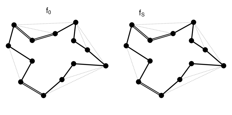
Our algorithm works as follows. Let be an input plane graph, and let be a cactus subgraph of whose triangles correspond to triangular faces of . The local search operation, -swap, is done as follows: As long as there is a collection of edge-disjoint triangles and such that contains more triangular faces of than and it remains a cactus, we perform such an improvement step. A cactus subgraph is called locally -swap optimal, if it can not be improved by a -swap operation. Remark that the triangles chosen by our local search are only those which are triangular faces in the input graph (we assume that the drawing of is fixed.)
Our analysis is highly technical, although the basic idea is very simple and intuitive. We give a high-level overview of the analysis. We remark that this description is overly simplified, but it sufficiently captures the crux of our arguments. Let be the solution obtained by the local search -swap algorithm. We argue that the number of triangles in is at least . We remark that the -swap is required, as we are aware of a bad example for which the -swap local search only achieves a bound of . For simplicity, let us assume that has only one non-singleton component. Let be the vertices in such a connected component.
Let be a triangle in . Notice that removing the three edges of from breaks the cactus into at most three components, say that are pairwise vertex-disjoint, i.e. sets are pairwise vertex-disjoint. Recall at this point that we would like to upper bound the number of triangles in by six times , where is the number of triangles in the cactus . Notice that is comprised of , where is the number of triangles in “across” the components (i.e. those triangles whose vertices intersect with at least two sets , where . Therefore, if we could somehow give a nice upper bound on , e.g. if , then we could inductively use where is the number of triangles in , and that therefore
and we would be done. However, it is not possible to give a nice upper bound on that holds in general for all situations. We observe that such a bound can be proven for some suitable choice of : Roughly speaking, removing such a triangle from would create a small “interaction” between components (i.e. small ). We say that such a triangle is a light triangle; otherwise, we say that it is heavy. Let be the current cactus we are considering. As long as there is a light triangle left in , we would remove it (thus breaking into ) and inductively use the bound for each . Therefore, we have reduced the problem to that of analyzing the base case of a cactus in which all triangles are heavy. Handling the base case of the inductive proof is the main challenge of our result.
We sketch here the two key ideas. Let . The first key idea is the way we exploit the locally optimal solution in certain parts of the graph . We want to point out; the fact that all triangles in are heavy is exploited crucially in this step. Recall that, each heavy triangle is such that its removal creates three components with many “interactions” (i.e. many triangles across components) between them. This large amount of interaction is the main reason why we could not use induction before. However, intuitively, these triangles across components could serve as candidates for making local improvements. So the fact that there are many interactions would become our advantage in the local search analysis.
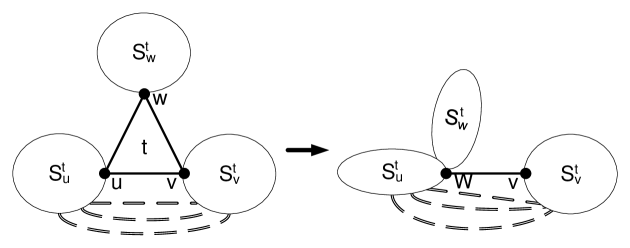
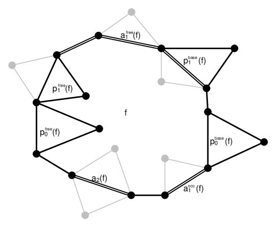
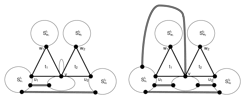
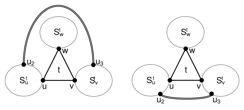
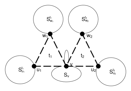
We briefly illustrate how we take advantage of heavy triangles. Let be the set of triangular faces in that are not contained in , so each triangle in has vertices in at least two subsets where . The local search argument would allow us to say that all triangles in have one vertex in , one in and one outside of . This idea is illustrated in Figure 2(a).
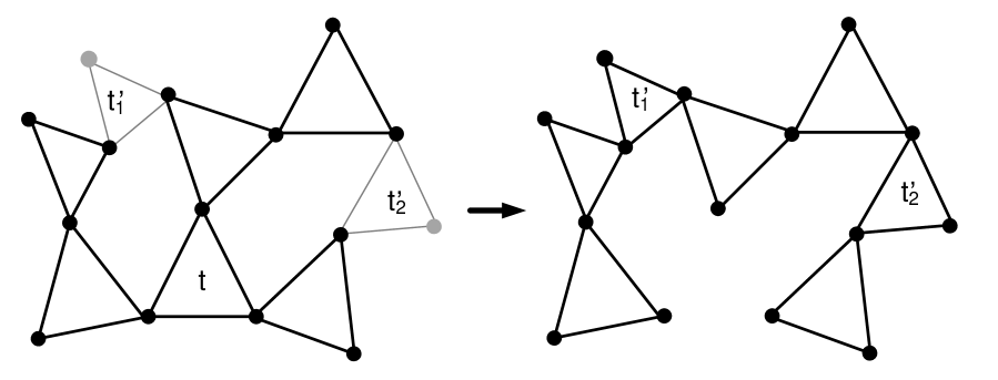
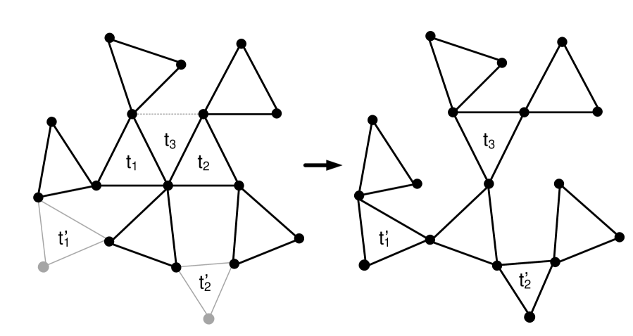
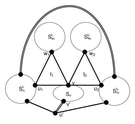
Moreover, we will argue that there are not too many triangular faces in , and we give a rough idea of how the exchange argument can be used in Figure 2(b).
Finally, the ideas illustrated in both figures are only applied locally in a certain “region” inside the input planar graph , so globally it is still unclear what would happen. Our final ingredient is a way to decompose the regions inside a plane graph into various “atomic” types. For each such atomic type, the local exchange argument is sufficient to argue optimally about the number of triangles in in that region compared to that in the cactus. Combining the bounds on these atomic types gives us the desired result. This is the most technically involved part of the paper, and we present it gradually by first showing the analysis that gives . For this, we need to classify the regions into five atomic types. To prove the main theorem, that , we need a more complicated classification into thirteen atomic types.
Organization of the paper:
In Section 2, we give a detailed overview of the proof. In Section 2.3, we show the inductive argument, reducing the general case to proving the base case. In Section 4, we show a slightly weaker version of the base case that implies , and in Section 5, we prove the base case to get our main result.
2 Overview of the Proof
In this section, we give a formal overview of the structure of the proof of Theorem 1.1. Let our input be a plane graph (a planar graph with a fixed drawing). Let be a locally optimal triangular cactus solution for the natural local search algorithm that uses -swap operations, as described in the previous section. Let denote the number of triangular faces of which correspond to the triangular faces of . We will show . In general, we will use the function to denote the number of triangular faces in any plane graph .
We partition the vertices in into subsets based on the connected components of , i.e. where is a connected cactus subgraph of . For each , where , let denote the number of triangular faces in with at least two nodes in . The following proposition holds by the -swap optimality of which implies .
Proposition 2.1
If for all , then .
Therefore, it is sufficient to analyze any arbitrary component where contains at least one triangle of (if the component does not contain such a triangle it is just a singleton vertex) and show that . Thus, from now on, we fix such an arbitrary component and denote simply by , by , and by . We will show that through several steps.
Step 1: Reduction to Heavy Cactus
In the first step, we will show that the general case can be reduced to the case where all triangles in are heavy (to be defined below). We refer to different types of vertices, edges and triangles in the graph as follows:
-
•
Cactus: All edges/vertices/triangles in the cactus are called cactus edges/vertices/triangles respectively.
-
•
Cross: Edges with exactly one end-point in are called cross edges. Triangles that use one vertex outside of are cross triangles. Notice that each cross triangle has exactly one edge in , that edge is called a supporting edge of the cross triangle. Similarly, we say that an edge supports a cross triangle; such a cross triangle contains exactly one vertex in some component . The component is called the landing component of . Similarly the vertex is called the landing vertex of .
-
•
type- edges: An edge in that is not a cactus edge and does not support a cross triangle is called a type- edge. An edge in that is not a cactus edge and supports cross triangle(s) is called a type- edge.
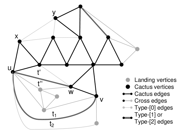
Therefore, each edge in is a cactus, type-, type- or type- edge. The introduced naming convention makes it easier to make important observations like the following (see Figure 3 for an illustration of our naming convention).
Observation 2.2
Triangles that contribute to the value of are of the following types: (i) the cactus triangles; (ii) the cross triangles; and (iii) the “remaining” triangles that connect three cactus vertices using at least one type-, type- or type- edge, and do not have a cross triangle drawn inside.
Types of cactus triangles and Split cacti:
Consider a (cactus) triangle in . For , we say that is of type- if exactly of its edges support a cross triangle. Let denote the number of type- cactus triangles, so we have that .
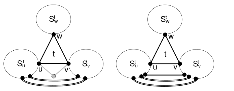
We denote the operation of deleting the edges of from a connected cactus by splitting at . The resulting three smaller triangular cacti (denoted by ) are referred to as the split cacti of . For each , let be the split component containing . Let . Denote by the set of type- or type- edges having one endpoint in and the other in . Now we are ready to define the concept of heavy and light cactus triangles, which will be crucially used in our analysis.
Heavy and light cactus triangles:
We say that a cactus triangle is heavy if either there are at least four cross triangles supported by or there are at least three cross triangles supported by the edges in one set for some and no cross triangle supported by the rest of the sets for each . Otherwise, the triangle is light. Intuitively, the notion of a light cactus triangle captures the fact that, after removing , there is only a small amount of “interaction” between the split components.
We will abuse the notations a bit by using instead of . Recall, that we denote by the total number of triangular faces in with exactly two vertices in . We denote by the total number of triangles in the cactus .
Function :
Consider a set and a drawing of (since we are talking about a fixed drawing of the plane graph , this is well-defined). Denote by the length of the outer-face of the graph . We define as the number of edges on the outer-face that do not support any cross triangle drawn on the outer-face, so we have .
The main ingredients of Step 1 are encapsulated in the following theorem.
Theorem 2.3 (Reduction to heavy triangles)
Let be a real number, and be as described above. If for all for which is a connected cactus that contains no light triangle, then for all .
Therefore, if we manage to show the bound for the heavy cactus, it will follow that in general (due to non-negativity of function ). In other words, this gives a reduction from the general case to the case when all cactus triangles are heavy. We end the description of Step 1 by presenting the description of .
Step 2: Skeleton and Surviving Triangles
Now, we focus on the case when there are only heavy triangles in the given cactus, and we will give a formal overview of the key idea we use to derive the bound , which in combination with Theorem 2.3, gives our main Theorem 1.1. For convenience, we refer to the terms and as simply and respectively.
Structures of heavy triangles:
Using local search’s swap operations, the light and heavy triangles behave in a very well structured manner. The following proposition summarizes these structures for heavy triangles (proof of this proposition in Appendix A.1).
Proposition 2.4
Let be a cactus triangle in cactus .
-
•
If is heavy, then is either type- or type-.
-
•
If is a heavy type- triangle and the edge supports the cross triangle supported by , then for all and the total number of cross triangles supported by edges in is greater than or equal to two.
-
•
If is a heavy type- triangle, then there is an edge such that for all and the total number of cross triangles supported by edges in is greater than or equal to three.
By Proposition 2.4 we can only have type- and type- cactus triangles in . Moreover, for each such heavy triangle , the type- or type- edges in only connect vertices of two split components of .
Let be the number of edges of type-. Notice that the number of non-cactus edges in is .
Skeleton graph :
Let be the set of all type- edges in and . Thus contains only cactus or type- or type- edges.
Each face of possibly contains several faces of , so we will refer to such a face as a super-face. At high-level, our plan is to analyze each super-face , providing an upper bound on the number of triangular faces of drawn inside , and then sum over all such to retrieve the final result. We call a skeleton graph of , whose goal is to provide a decomposition of the faces of into structured super-faces. Denote by the set of all super-faces (except for the faces corresponding to cactus triangles).
Let be a super-face. Denote by the number of triangular faces of drawn inside that do not contain any cross triangles. Now we do a simple counting argument for using the skeleton as follows: (i) There are cactus triangles in , (ii) There are cross triangles supported by edges in , and (iii) There are triangular faces in that were not counted in (i) or (ii). Combining this, we obtain:
| (1) |
The first and second terms are expressed nicely as functions of ’s and ’s, so the key is to achieve the best upper bound on the third term in terms of the same parameters. Roughly speaking, the intuition is the following: When or is high (there are many edges in supporting cross triangles), the second term becomes higher. However, each cross triangle would need to be drawn inside some face in , therefore decreasing the value of the term . Similar arguments can be made for . Therefore, the key to a tight analysis is to understand this trade-off.
The structure of super-faces:
Let be a super-face. Recall that an edge in the boundary of is either a type- or type- edge, or a cactus edge. We aim for a better understanding of the value of . In general, this value can be as high as , e.g. if is a triangulation of the region bounded by the super-face using type- edges. However, if some edge in the boundary of supports a cross triangle whose landing component is drawn inside of in , this would decrease the value of , by killing the triangular face adjacent to it, hence the term .
The following observation is crucial in our analysis:
Observation 2.5
Consider each edge . There are two possible cases:
-
•
Edge is a type- or type- or cactus edge and supports a cross triangle drawn in .
-
•
Edge is a type- or type- or cactus edge and does not support any cross triangle drawn in .
Edges lying in the first case are called occupied edges (the set of such edges in is denoted by ), while the others are called free edges in (the set of free edges in is denoted by ). The length of can be written as .
A very important quantity for our analysis is , roughly bounding the value of (within some small constant additives terms.)
We will assume without loss of generality that is the maximum possible value of surviving triangles that can be obtained by drawing type- edges in , so is a function that depends only on the bounding edges in . We define , which is again a function that only depends on bounding edges of . Intuitively, the higher the term , the better for us (since this would lower the value of ), and in fact, it will later become clear that roughly captures the “effectiveness” of a local exchange argument on the super-face . Hence, it suffices to show that is sufficiently large. The following proposition makes this precise:
Proposition 2.6
Proof.
Notice that can be analyzed as follows:
-
•
Each cactus triangle is counted three times (once for each of its edges), and for a type- triangle, one of the three edges contribute only one half. Therefore, this accounts for the term .
-
•
Each type- or type- edge is counted two times (once per super-face containing it in its boundary). For a type- edge, the contribution is always half (since it always is accounted in ). For a type- edge, the contribution is half on the occupied case, and full on the free case. Therefore, this accounts for the term .
Overall we get, , which finishes the proof. ∎
Combining this proposition with Equation 1, we get:
| (2) |
A warm-up: Using the gains to prove a weaker bound:
To recap, after Step 1 and Step 2, we have reduced the analysis to the question of lower bounding . We first illustrate that we could get a weaker (but non-trivial) result compared to our main result by using a generic upper bound on the gains. In Step 3, we will show how to substantially improve this bound, achieving the ratio of our main Theorem 1.1 which is tight.
Lemma 2.7
For any super-face (except for the outer-face) in , we have .
As the outer (super-)face of is special, we can achieve a lower bound on the quantity that depends on . This is captured by the following lemma.
Lemma 2.8
For the outer-face , we have that .
| (3) |
The following lemma upper bounds the number of skeleton faces (i.e. super-faces of the skeleton.)
Lemma 2.9
.
Proof.
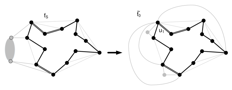
Proposition 2.4 allows us to modify the graph into another simple planar graph such that the claimed upper bound on will follow simply from Euler’s formula.
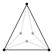
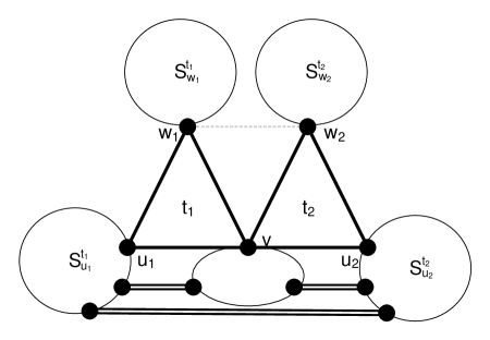
Let be a cactus triangle where and be such that the edge set is empty, as guaranteed in Proposition 2.4. For every cactus triangle we contract the edge into one new vertex . Note that this operation creates two parallel edges with endpoints and in the resulting graph. To avoid multi-edges in the resulting graph we remove one of them (see Figure 4 for an illustration of this operation). Since is empty this operation cannot create any other multi-edges in . In addition the contraction of an edge maintains planarity, hence after each such transformation the graph remains simple and planar. As a result of applying the above operation to all cactus triangles, the graph has vertices and edges corresponding to the contracted triangles. By Euler’s formula the number of edges in is at most , which implies that , and as we get that . ∎
Step 3: Upper Bounding Gains via Super-Face Classification
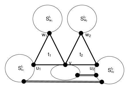
In this final step, we show another crucial idea that allows us to reach a factor . Intuitively, the most difficult part of lower bounding the total gain is the fact that the value of is different for each type of super-face, and one cannot expect a strong “universal” upper bound that holds for all of them. For instance, Figure 5 shows a super-face with , so strictly speaking, we cannot improve the generic bound of .
This is where we introduce our final ingredient, that we call classification scheme. Roughly, we would like to “classify” the super-faces in into several types, each of which has the same gain. Analyzing super-faces with similar gains together allows us to achieve a better result.
Super-face classification scheme:
We are interested in coming up with a set of rules that classifies into several types. We say that the rule is a -type classification if the rules classifies into sets . Let be a vector such that . We would like to prove a good lower bound on the gain for each such set. We define the gain vector by where . The total gain can be rewritten as:
Notice that, the total gain value would be written in terms of the variables, so we would need another ingredient to lower bound this in terms of variables ’s and ’s. Therefore, another component of the classification scheme is a set of valid linear inequalities of the form . This set of inequalities will allow us to map the formula in terms of into one in terms of only ’s and ’s.
A classification scheme is defined as a pair . We say that such a scheme certifies the proof of factor if it can be used to derive . Given a fixed classification scheme and a gain vector, we can check whether it certifies a factor by using an LP solver (although in our proof, we would show this derivation.)
Our main result is a scheme that certifies a factor . Since the proof is complicated, we also provide a simpler, more intuitive proof that certifies a factor first.
Theorem 2.10
There is a -type classification scheme that gives a factor .
We remark that the analysis of factor only requires a cactus that is locally optimal for -swap.
Theorem 2.11
There is a -type classification scheme that gives a factor .
Intuition:
The classification scheme would intuitively set the rules to separate the super-faces that would benefit from local search’s exchange argument from those that would not. Therefore, for the good cases, we would obtain a much better gain, e.g., in one of our classification type, is as high as . In the bad cases that there is no such benefit, we would still use the lower bound of that holds in general for any super-face.
3 Reduction to Heavy Cacti (Proof of Theorem 2.3)
Let be a light triangle. Assume that the bound holds for all where contains only heavy triangles. Our goal is to prove that it holds for all . We will prove this by induction on the number of light triangles contains. The base case (when all triangles are heavy) follows from the precondition and the trivial base case when is clearly true. Now assume that there is a light triangle in the in graph . Our plan is to apply the induction hypothesis on the subgraphs since each contains less light triangles than .
Since we will be dealing with light triangle , the following proposition (proof in Appendix A.2) gives some important structural properties of such a triangle:
Proposition 3.1 (Structure of light triangles)
Let be a light triangle in . The following statements hold:
-
•
If is a light type- triangle and , such that for all , then the total number of cross triangles supported by edges in is at most two.
-
•
If is a light type- triangle and the edge supports the cross triangle supported by and for all , then the total number of cross triangles supported by edges in is at most one.
-
•
If is a light triangle where edges in support either two or three cross triangles such that at least two different set of edges for supports a cross triangle each, then each set of edges supports at most one cross triangle and all the supported cross triangles have the same landing component.
We will also need the following observation.
Observation 3.2
Any circuit in , which comprises of only cactus, type-, type- and type- edges and cactus vertices, divides the plane into several regions (two if is a cycle) such that any cross triangle which is drawn in one of the regions cannot share its landing component with any other cross triangle drawn in some different region.
Free and occupied edges:
We call the edges in the outer-face of that contribute to free and every other edge in that is not free is called occupied. Let be the total number of occupied edges. It follows that .
3.1 Inductive proof
Now we proceed with the proof. Consider a cactus triangle with which is light. To upper bound , we break it further into two distinct terms :
The term counts all triangles with all the three vertices in the same split component and the cross triangles supported by edges or triangles in for some . As each split component of is also a cactus subgraph, by induction we have for for all : . and as is equal to the sum over for all we get
The term counts all remaining triangles in , i.e. the triangles whose vertices belong to at least two different split components of . We will proceed to show that
hence, upper bounding by the desired quantity for any .
To this end, we upper bound the contributions to from two separate terms: The first term, , is the number of cross triangles supported by the edges in plus the cross triangles supported by plus one for itself, and (ii) The second term, , is the number of “surviving” triangular faces in without any cross triangle drawn inside it.
Note that by definition of light triangles, there are at most three cross triangles supported by the edges in and itself. Now we consider two cases, based on the value of .
-
•
(At most two supported cross triangles): In this case , i.e. itself and the supported cross triangles. Hence if we can show that , then we are done.
-
•
(Exactly three supported cross triangles): Similarly in this case , i.e. itself and the supported cross triangles. Hence showing that gives us the entire reduction.
In particular, the following lemma (which we spend the rest of this section proving) will complete the proof of Theorem 2.3.
Lemma 3.3
For any light triangle , the number of surviving triangles is at most . Moreover, if there are three cross triangles supported by the edges in and itself, then is at most .
3.2 Proof of Lemma 3.3
To facilitate the counting arguments that we will use, we will be working with an auxiliary graph instead of . Let be the cycle (in particular, the set of edges on the cycle) bounding the outer-face of for and let be the cycle bounding the outer-face of (so contains exactly all the outer-edges). Because is a connected triangular cactus, there cannot be any repeated edge in these faces, hence , ’s are circuits; the vertices can occur multiple times in . Now we cut open each of the circuits ,, for each to convert them to simple cycles. The idea is to make copies (equal to the number of times it appears in the corresponding circuit) of each vertex contained in the circuit and joining the edges incident to the original vertex to one of the copies, such that the structure of the drawing is preserved. We also make sure that there exists a triangular face corresponding to containing some copy of each of the vertex in . After cut opened, , for each will be empty cycle in . Notice that the values of as well as the types of edges on these cut-opened cycles are preserved.
Note that the surviving triangles that contribute to correspond exactly to the triangles drawn in the regions of exterior of for all but in the interior of . Also, is drawn inside of . In order to bound we construct an auxiliary graph as follows. For each , we remove all edges and vertices drawn in the interior of cycle from . The resulting graph after such a removal is our , such that . Any triangle that contribute to the term also exist as triangular faces in , so we only need to upper bound .
Claim 3.4
If , then the bound for holds.
Proof.
If the set is empty, then and in general. In the three cross triangles case, having no such edge implies that is a type- triangle, because all the three cross triangles has to be supported by and hence . ∎
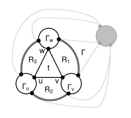
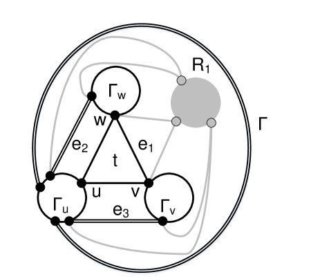
Now we continue with the case where there exists at least on edge in . Clearly, is a subgraph of and any surviving triangle in must be drawn in a region of . In order to bound the number of surviving triangles corresponding to , we will first identify these regions and then make a region-wise analysis to get the full bound. For this purpose, we remove any non-cactus edge from that is drawn in the interior of and does not belong to one of or to form another auxiliary graph . The faces in the graph which are drawn inside the cycle and outside every cycle (except the triangular face ), will correspond to the regions in which we would analyze later. First we prove the following claim which quantifies the structure of these regions (see Fig. 6 which illustrates all possible structures for these regions).
Claim 3.5
If (except the triangular face ) are the faces in which are drawn inside and outside every cycle for each , then . Moreover, every such face contains exactly one edge of .
The proof of this claim appears later in this section.
Let (for ) be the regions in which are the faces of given by the above claim (see Figure 6 for an illustration). We denote by 777Notice that we slightly abuse the notation here. Before, we use where is a subset of cactus-vertices, and now we are using where is a cycle bounding a region. the overall number of edges and by the number of occupied edges in the boundary of (these are the edges belonging to some cycle for .) In the next step, we will upper bound the number of surviving triangles that exist in in each such region .
Observation 3.6
Any face in the graph which is drawn inside one of the regions contains vertices from at least two cycles for and .
How many surviving triangles can there be in region ? Intuitively, if we triangulate by adding edges in its interior, we would have triangular faces. Among these faces, of them would not be surviving since the edge bounding the face is occupied. In certain cases, we would get an advantage and the term would become instead of .
Claim 3.7
The number of surviving triangles drawn inside in are at most . Moreover, if the common landing component for the three cross triangles supported by is drawn inside , then we get the stronger bound of .
The proof of this claim relies on a standard triangulation trick used in the context of planar graphs. We defer the proof to later in Section 3.4.
Now we are ready to complete the proof for Lemma 3.3.
Let be the indicator variable such that if we are in the case when there exists exactly three cross triangles supported by such that the common landing component for these triangles is drawn inside some region , otherwise . Using the bounds for each region from Claim 3.7 we can upper bound by summing over the number of surviving triangles in each region.
| (4) |
Next we take a closer look at the term in the sum. By Claim 3.5, each region contains exactly one edge of , and . Therefore, we can decompose the length of face into three parts:
Plugging this into Eq. (3.2) we get,
| (5) | ||||
| (6) |
Note that can not contribute more than its three edges to the boundaries of all regions, thus . Using this in Eq (5), we get
| (7) |
Claim 3.8
Proof.
Notice that the sum on the left-hand-side counts all edges in where each edge is counted exactly once, and this contribution is . Additionally, by Claim 3.5, each edge in is also counted exactly once as well, and this contribution is . ∎
Combining all of this with Inequality (7) we get,
| (8) |
Let be the number of occupied edges among the occupied edges belonging to such that they do not belong to any of the for . These edges are the ones which are drawn across two different cycles for and (potentially some of the edges drawn in double-line style in Fig. 6). Hence captures precisely the number of occupied edges in for which the supported cross triangles are drawn in the exterior of . By the way we define , the following equality holds.
| (9) |
Using this in Inequality (8) we get,
Since for every we get,
| (10) |
The general inequality for the Lemma 3.3 trivially follows from the above inequality. The following claim will complete the proof.
Claim 3.9
If there are three cross triangles supported by edges in with the common landing component , then .
Proof.
There could be two sub-cases: (i) The landing component is in the exterior of . In this case, by the definition of , all the three edges which support one of the three cross triangles will contribute to (see Fig 7 for illustration); and (ii) The cross triangles are drawn inside . In this case, we have that . In any case, we have , thus proving the lemma. ∎
3.3 Proof of Claim 3.5
By the assumption that there exists at least one edge in . Let be one such edge.
To prove the claim, we will show that for any such edge, there exists a unique face satisfying the conditions of the claim and it contains at least one edge from . As each edge of is also incident to the face bounded by , this would imply that there can not be more than three such faces in and since there exists the edge , hence we will be done.
Let for some . We will always use the fact that, since , there are two directions starting from to traverse the boundary of , such that in one direction edges of belongs to and in the other they are drawn in the interior of . No we split into two possible cases.
-
•
( for some such that ): Since , there exists a path from to containing edges of such that all these edges are drawn in the interior of (possibly and is a zero length path). Similarly there exist a path going from to containing edges of such that all these edges are drawn in the interior of . Hence the circuit which includes the edge , the edge and two paths and , is drawn inside of (except the edge which is on the boundary of ). Clearly, there cannot be any other edge from which is drawn inside , hence any face drawn inside can contain at most the edge from . Also, by the way we define , there cannot be any other edge inside drawn across different cycles. Now if is drawn outside of , then itself is the face of satisfying our requirements. Otherwise, the whole of for and , is drawn inside of . This means that region inside the circuit can be decomposed into the triangular face , the cycle and another face whose boundary comprises of edges , the edge of , the edge and two paths and . Hence is the face corresponding to which we require.
-
•
(): Notice that in this case, the circuit comprising of edge along with a path from to containing edges of such that all these edges are drawn in the interior of , will enclose the triangle and the other two cycles such that and . Similar to the previous case, there cannot be any other edge from which is drawn inside , is drawn in the interior of (except the edge which is on the boundary of ) and also no other edge is drawn across different cycles inside of . Hence, any face drawn inside can contain at most the edge from . Also, can be decomposed into the triangular face , the cycles and another face whose boundary comprises of edge , all three edges of , all the edge of and two paths and from to and to containing edges of drawn inside . Hence is the face corresponding to which we require.
3.4 Proof of Claim 3.7
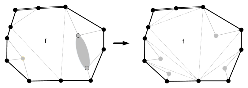
To prove this we will perform a series of monotone operations within the region in graph , such that in each operation the number of surviving triangles drawn within cannot reduce. In the end we will reach a structure for which the bound holds trivially. Since the operations here are monotone, the bound which we get also holds for the original number of surviving triangles drawn within . Notice that we make these modifications in the auxiliary graph only for counting purposes and never change the structure of our graph .
In the first step, except for the three cross triangles supported by the edges in , we decouple all the other supported cross triangles drawn inside which share their landing components by adding a dummy landing vertex for each such cross triangles and making the new dummy vertex its landing component. Note that the decoupling step allows us to get a full triangulation for in its interior (except the face containing the common landing component ) and at the same time does not affect the number of surviving triangles drawn inside in .
After this we triangulate the interior of by adding extra type- edges, such that the end point for each additional edge lies in two different and for . This is possible to achieve due to Obs. 3.6 and also this operation is monotone and cannot reduce the number of surviving triangles drawn inside in . Also, all the faces inside are triangular faces except the one containing in graph . The way we triangulate the regions of ensures that the Obs. 3.6 continues to hold which implies that any face in can contain at most one edge from the boundary of for any . Also, will remain a simple planar graph since the added type- edge connect vertices from the boundary of two different cycles and for . In the end, we have at most triangular faces and any occupied edge counted in (i.e. occupied edges in which belongs to some cycle for ) can kill at most one triangle, hence the claimed upper-bound follows in the general case.
Now in the case where we have the three cross triangles supported by the edges in , we will prove that the face (say ) of inside which the common landing component is drawn, contains at least one more edge in addition to the three edge from which supports the three cross triangles. This implies that this face has length at least and the triangulation of misses at least triangular faces. Also, in the worst case the fourth edge which we consider here could contribute to the term . Hence overall, we get at least less surviving triangular face than the previous bound and the claim follows.
To prove the claim for face , first recall that (by Prop. 3.1) the three edges in which supports the cross triangles are drawn across different pair of cycles . Let , and be the three edges supporting the three cross triangles. There is a cycle comprising of edges and paths joining the two ends of these edge in respectively, such that the triangle is drawn inside and the exterior of the is outside of . Now since is a bounded region in graph hence the face is a bounded face. Now we show that for to be bounded face, its length has to be at least four. In the corner case when , is precisely the triangular face and the edges are are touching from the outside of . Hence, for to be bounded, there should exist at least one more edge to complete the loop going from to to and back to to . Otherwise, assume (other cases are symmetric). Since the cross triangles supported by share their landing component, and there exists a cycle containing only cactus/type-/type-/type- edges including edges , and paths in and connecting the end points of and , such that the face should be drawn outside of . Now again for to be bounded, it should contain one more edge and we are done.
4 Classification Scheme for Factor
In this section we will show a classification scheme that allows us to prove our factor seven result. For simplicity, from now on we will use instead of . More precisely, the aim is to prove the following lemma.
Lemma 4.1
There is a -type classification scheme for which
First, we show that Lemma 4.1 is sufficient for proving the final result. For this we substitute the bound from Lemma 4.1 into Inequality (2) to get:
This implies as desired.
In order to define the classification schemes, we further classify the edges, vertices and split components for any heavy triangle in into several types.
Further classification of cactus vertices, edges and split components:
The cactus edges on each heavy triangle are further classified into free and base edges as follows: For any heavy triangle , where . Let be an edge for which . By Proposition 2.4 there is exactly one such edge in . We say that the edge is the base edge and both and are called base vertices. We say that the other two edges in are free, and the vertex is called a free vertex. Both and are called occupied components and is a free component. See Figure 9 for an illustration.
The following claim follows from the properties of heavy type- and type- triangles shown in Proposition 2.4.
Claim 4.2
The two free cactus edges of any cactus triangle are part of the same super-face in .
Proof.
Let and be the free edges in . Assume for contradiction that there is a super-face that only contains but not . Any super-face boundary needs to contain at least one type- or type- edge in order to form a cycle. Therefore a path along the super-face , not including the edge , from to must leave using a type- or type- edge, a contradiction to the fact that for a heavy triangle, and are empty in graph . ∎
We will upper bound the number of surviving triangles inside each super-face based on the characteristics of the edges bounding (see Figure 10).
Classification of Edges in the Face Boundaries of :
Edges that bound are further partitioned into the following types:
-
•
The two free edges of the cactus triangles. Let and denote the total number of type- and type- triangles respectively whose free edges participate in .
-
•
The base edges of the cactus triangles. Let and denote the total number of such triangles whose base edges participate in .
-
•
The type- edges. Let denote the total number of such edges on .
-
•
The type- edges whose supported cross triangle are drawn inside . This side of any type- edge is referred to as the occupied side. Let denote the total number of such edges in the boundary of .
-
•
The type- edges whose supported cross triangle is drawn in in some region bounded by a super-face other than . This side of any type- edge which does not support a cross triangle is referred to as the free side. We denote the number of such edges by .
Notice that , since all cactus triangles in are heavy, hence . Since is a triangular cactus and , the following can be observed.
Observation 4.3
For any super-face , .
Let , and .
Observation 4.4
Any surviving triangular face cannot be incident to any type- edge, the occupied side of a type- edge or the base side of a type- triangle.
4.1 Classification Rules
Now we are ready to define the classification rules for our analysis. Since the bound on the number of surviving triangles (hence the quantity) that can be drawn inside each super-face heavily depends on the type of edges contained in its face boundary, we classify each super-face (except the outer-face ) into three broad categories, based on the total number of edges. We also sub-categorize each super-face for which into further classes, based on whether it contains an edge or not.
Classifications of super-faces:
A super-face will be of type- if and . If there is no restriction on some dimension, then we put a dot () there. Following is the precise categorization for the super-faces in .
-
•
A super-face is of type-), if in addition
-
–
is of type- , if or
-
–
of type-), if .
-
–
-
•
A super-face is of type-, if
-
•
A super-face is of type-, if
Let the set be the subset of type- super-faces in and analogously let for each type- super-face. Notice that and for any , which implies, . Also, for any , hence, .
The following lemma (whose proof will appear in Section 4.3) gives lower bounds on the quantity for each type of super-faces in . For we will use Lemma 2.8 (whose proof will appear in Section 4.4).
Lemma 4.5
For any super-face , the following holds:
-
1.
If is of type-), then .
-
2.
If is of type-), then .
-
3.
If is of type-), then .
-
4.
If is of type-), then .
4.2 Proof for Lemma 4.1
Notice that the bounds for type- and type- are better than the trivial bound of , which leads to the improvement from to .
We apply Lemma 2.8 and Lemma 4.5 to , depending on the type of each super-face: In particular, this includes the lower bounds for each super-face of type-, type-, type-, type- and the outer-face .
Here we use the fact that .
| (11) |
Next, we deal with the “residual terms” highlighted in the formula above by the box. For this purpose, we present various upper bounds on the number of super-faces of certain type:
Lemma 4.6 (Two upper bounds on the number of super-faces)
The following upper bounds hold:
-
1.
.
-
2.
.
Proof.
We start by proving the first upper bound. Since for a type- super-face and each type- edge can contribute to to exactly one super-face in , we have that .
The second upper bound can be proved by a simple charging argument. On each super-face , we give unit of money to a certain set of edges on the face. In particular, each of the following types of edges gets a unit: (i) base of the type- cactus triangle, (ii) type- edge, and (iii) type- edge. Therefore, the total amount of money put into the system is exactly:
Counting from a different viewpoint, each super-face of type- receives at least units of money, so the total amount is at least . This immediately implies the inequality:
∎
Using equality in Inequality (4.2), we get:
| (13) |
4.3 Handling the Non-Outer-Faces (Proof of Lemma 4.5)
We split the proof of Lemma 4.5 into three parts. First we show an upper bound for the number of surviving triangles if a super-face has or . Then we show that , if and . Finally we combine both results to give the upper bound for the number of surviving triangles in each type of super-face in .
Lemma 4.7
Let , if or we have
Proof.
If and , it is easy to enumerate all possible compositions of the face boundary of and check for each case that the claimed bound holds.
-
•
(:) In this case, , and .
-
•
(:) In this case, , and .
-
•
(:) In this case, , , and .
Now consider the case where . In order to bound in this case, we locally modify the internal structure for a fixed in a special way. Notice that we make these modifications only for counting purposes and they do not change the structure of our graph in any way. First we decouple the supported cross triangles drawn inside which share their landing components by adding a dummy landing vertex for each such cross triangle and making the new dummy vertex its landing component. Then using additional type- edges we triangulate the super-face in an arbitrary way. Note that the decoupling step allows us to get a full triangulation for and at the same time this operation does not reduce the value of for (see Figure 11 for illustration). Hence, any bound which we get after performing this operation also holds for the original quantity . This triangulation of the super-face has exactly triangular faces. Starting with this bound, we use the particular structure of to achieve the desired bound for .
By Observation 4.4 no edge of type-, occupied side of a type- edge or base side of a type- triangle can be adjacent to any triangular face in . Also, at most two of these edges could belong to any triangular face in . Hence, out of all the potential faces in the triangulate super-face , at least faces will be killed and hence we get the claimed bound on . ∎
For other cases, we can still get a slightly weaker bound.
Lemma 4.8
Otherwise, if and , then we have
Proof.
Notice that implies . Hence the first inequality is trivially true by substituting the value and . ∎
4.4 Handling the Outer-Face (Proof of Lemma 2.8)
In this section we will prove that . If , this bound can be easily achieved by enumerating all possible compositions of the face boundary of . If , the term in the bound we want to prove becomes more significant and hence this case needs special treatment.
In contrast to the other super-faces in , the number of surviving triangles in also depends on . We first give an intuition on how this term influences the number of surviving triangles in and then use the idea behind it to prove Lemma 2.8. Starting from , we can construct an auxiliary graph by modifying the outer-face , such that this part of the graph is fully triangulated using type- edges, such that in total we obtain extra triangles. Also, in this process the structure of the free and occupied edges of the outer-face (say ) of the subgraph (where is the set of type- edges) of remains exactly the same as that of the original outer-face of . Finally, we use the trivial upper bound given by Lemma 4.7 on the number of triangular faces drawn inside the outer-face in graph , which in turn gives us the term for the bound on the number of triangular faces drawn inside the outer-face in graph . Notice that the modified graph is created only for counting purposes and the modification does not change the structure of our original graph in any ways.
The following lemma formalizes this idea of triangulating the outer-face.
Lemma 4.9
For the graph with outer-face having free edges, there exists another simple planar graph with outer-face , such that
-
•
The graphs and only differ inside the outer-face of .
-
•
The structure of the outer-face for the graph (where is the set of type- edges) is the same as that of , i.e. and .
-
•
There are at least extra surviving triangles drawn inside the outer-face in as compared to the outer-face in .
Proof.
In order to prove this lemma, we will transform to by creating at least new surviving triangles in by first pre-processing and then triangulating using extra type- edges in a specific way.
First we decouple the supported cross triangles drawn inside which share their landing components by adding a dummy landing vertex for each such cross triangle and making the new dummy vertex its landing component. Notice that the decoupling step makes the induced graph an outer-planar graph, where are the vertices contained in face . Also, it does not change the structure of the graph anywhere else except inside face . Since is outer-planar, there exists a vertex , such that the degree of in is two. Now we number the vertices in the face in clockwise order as , where is the degree vertex in . Next we triangulate the outer-face by adding a star of type- edges with vertex as the root for this star and vertices as the leaves of the star (see Figure 12). This completes the construction of our auxiliary graph . Notice that this operation cannot create a parallel edge in , implied by the way we fixed . Also, the decoupling and triangulation will maintain the planarity of . Finally, it is easy to see that the occupied and the free edges for the outer-face of graph are the same as that of the original outer-face , hence the second property is satisfied.
Each of the triangles and could either survive if both the edges coming from are free or not survive if at least one of these edges is occupied. Any triangle of the form for will survive if the edge is free. Now if both the triangles and do not survive, then at most two out of the free edges can be a part of these triangles and hence there will be at least triangles of the form for which survive. If one of the triangles and survives, then at most three out of the free edges can be part of these triangles and hence there will be at least triangles of the form for which survive. Else both of the and triangles survive, then four out of the free edges will be part of these triangles and hence there will be at least triangles of the form for which survive. Hence, overall in each case, triangles survive and the lemma follows. ∎
Note that consists of a subset of the edges counted in and . Also , since is formed after including all the edges drawn inside in (see Figure 13).
Now, we are ready to present the proof of Lemma 2.8. We split the analysis into two cases:
-
•
First, consider the case when . The worst case then is when , which implies , and . In this case, , which gives the inequality.
Otherwise, when , we have (there would be an occupied edge that supports a cross triangle in which kills it), and . This gives , and .
-
•
From now on we assume that . For this case, we use Lemma 4.9 on to get the auxiliary graph with at least extra surviving faces in its outer-face, totaling to . Now using the trivial bound given by Lemma 4.7 on the outer-face for the corresponding graph , we get
which proves the lemma.
Intuition for next step
The tight example (see Appendix B.1) of the factor analysis for a -swap optimal solution shows that looking at a locally optimal solution for -swap is not enough to achieve our main Theorem 1.1. In this example there exists an improving -swaps, which indicates that further classification of super-faces in and achieving stronger bounds for some special type of super-faces (which we refer to as type-, type- and type- super-faces) could lead to an improvement. These special super-faces are the ones where an adversary can efficiently packs a lot of surviving triangles which leads to . It turns out that in every such super-face, there is an improving- swap. Hence to prove the tight bound, it is necessary to get stronger bounds for such faces by looking at locally optimal solution for -swaps. This intuition lead us to the sub-categorization of the type- and type- faces in .
5 Classification Scheme for Factor
We will show a classification scheme that certifies the factor . This scheme extends the one given in the previous section.
5.1 Classification Rules
The important observation that leads to a better bound is to derive a better gain for super-faces of type- and type- in the previous classification. We notice that, for a certain sub-class of these super-faces, a better bound can be obtained.
A New Super-face Classification:
Now we sub-categorize type- and type- super-faces into further classes, based on the values of and . A super-face will be of type- if , and . If there is no restriction on a particular dimension, then we put a dot () there. Following is the categorization of super-faces which we use.
-
•
type-:
-
–
type-:
-
*
type-:
-
*
type-:
-
*
-
–
type-:
-
*
type-:
-
*
type-:
-
*
-
–
-
•
type-:
-
–
type-:
-
*
type-:
-
*
type-:
-
*
-
–
type-:
-
–
type-:
-
–
-
•
type-:
Let the subset be the set of type- super-faces and analogously let . It is easy to see that the categorization partitions the set , for any , which implies, . Also, for each , for each .
We classify a sub-class of type-, type-, and type- super-faces that admits an improved bound via several new notions.
Adjacent triangles and edges and friends:
Let and be two cactus triangles that share a vertex. Denote their vertices by , where (say ). In this case, we call them adjacent triangles. Let be a free vertex of . If there is a way to draw an edge such that the region bounded by is empty, we say that these triangles are strongly adjacent; otherwise, they are weakly adjacent. Furthermore, if the and are strongly adjacent in and , then we say that and are friends or friendly triangles.
Observation 5.1
The free sides for any pair of triangles which are strongly-adjacent or friends are part of the same super-face in .
We will crucially rely on the following lemma, whose proof is provided later in Section 5.5
Lemma 5.2 (Friend Lemma)
The following properties hold:
-
•
No type- heavy triangle is friends with any other heavy cactus triangle.
-
•
For any pair of type- triangles which are friends, their corresponding base sides belong to a common super-face in .
From the lemma, whenever we talk about friends, we always mean a pair of type- triangles.
Friendly super-faces:
We call a super-face of type- or a friendly super-face if it contains at least one pair of cactus triangles that are friends. Let , and be the set of friendly super-faces of type- and respectively. Also, let . Let .
The subsequent lemmas (which we prove later) give us stronger bounds on for super-faces of type- or which are not friendly.
Lemma 5.3
For any type- super-face , the following bound holds for .
Lemma 5.4
For any type- super-face , the following bound holds for .
Lemma 5.5
For any type- super-face , the following bound holds for .
Now, we have identified the set of super-faces for which we obtain an improved bound. The rest of the super-faces only relies on trivial upper bounds.
Lemma 5.6
For any super-face , the respective bounds hold for
-
•
type-:
-
•
():
-
•
type-:
-
•
():
-
•
type-:
-
•
():
-
•
type-:
-
•
type-:
-
•
type-:
5.2 Valid Inequalities
We present various upper bounds on the number of super-faces of certain type. We denote by the following system of linear inequalities.
Lemma 5.7 (Various upper bounds on the number of super-faces)
The following bounds hold:
-
•
-
•
-
•
Proof.
The first bound is derived in exactly the same manner as in Lemma 4.6. The second bound is also similar. Consider the sum:
Notice that each super-face of type- or type- gets the contribution of at least , while the other type gets the contribution of , so we have that the sum is at least .
Finally, for the third bound, we give a combinatorial charging argument. First, we imagine giving unit of money to each type- triangle. Therefore, units of money are placed into the system. We will argue that we can “transfer” this amount such that each super-face in receives at least one unit of money, hence establishing the desired bound.
-
•
For each face , we know that there must be at least one pair of friends. By Lemma 5.2, no type- triangle is friends with any other heavy cactus triangle. The super-face receives unit of money from each such triangle in the pair, so we have units on each such super-face.
-
•
Now consider a super-face . On such super-face, there is at least one type- triangle, and such cactus triangle would (i) pay super-face if it still has the money, or (ii) the “extra” money would be put in the system to pay if no cactus triangle in has money left with it.
In the end, all such super-faces would have at least one or two units of money, so the total money in the system is at least . The total payment into the system is at most plus the extra money. There can be at most units of extra money spent: Due to Lemma 5.2, i.e. whenever a face contains a triangle that spent in the first step, it must also contain its pair of friends, so there can be at most such faces that cause an extra spending. This reasoning implies that
∎
Deriving Factor 6:
Now that we have both the inequalities and the gain bounds, the following is an easy consequence (e.g. it can be verified by an LP solver.) For completeness, we produce a human-verifiable proof in Appendix A.3.
Lemma 5.8
5.3 Gain analysis for other cases
In this section, we analyze the gain for various types of faces where we get improved bounds.
5.3.1 Super-faces (Proof for Lemma 5.3)
A super-face in this set turns out to behave in a very structured way, i.e. the edges of the cactus triangles bounding this face look like a “fence”, which is made precise below.
Cactus fence:
A cactus fence of size is a maximal sequence of cactus triangles such that any pair and are strongly adjacent. Moreover, for each triangle , if is a free vertex of , then is a singleton.

Lemma 5.9 (Fence lemma)
Any super-face is bounded by free sides of a cactus fence together with one edge that is of type-.
The proof of this lemma is quite intricate and is deferred to the next subsection. Moreover, from definition of the set , each pair of cactus triangles on this face is not a pair of friends. It suffices to show that : Since , this would imply which proves the lemma.
For obtaining the bound on , we obtain an auxiliary graph on by modifying the inside of the super-face . First we decouple the supported cross triangles drawn inside which share their landing components by adding a dummy landing vertex for each such cross triangle and making the new dummy vertex its landing component. Then the inside of is fully triangulated using additional type- edges such that in total it contains triangular faces. Notice that, this process cannot decrease the number of triangles drawn inside of in .
Lemma 5.10
If a super-face contains a single cactus fence structure and only one additional edge, then any triangulation of using type- edges must contain the free sides for at least one pair of cactus triangles which are friends.
Proof.
The lemma follows easily using the facts that in any triangulation of a polygon there are at least two triangles each containing two side of the polygon and no two base vertices can be joined by an edge inside super-face as this will create a multi-edge, hence there should be at least one triangular face containing two adjacent free edges each belonging a different cactus triangle from a pair of strongly adjacent cactus triangles. ∎
It is clear that , hence by Lemma 5.10, contains an edge joining strongly adjacent pair of cactus triangles. Hence, but not drawn inside in (since cannot contain any pair of friends), so still contains all surviving faces in the original graph and has only triangular faces inside . Since the friends edge goes across the two free vertices of two cactus triangles but joins two base vertices of two cactus triangles, hence they cannot form a triangle together. This implies at least one more triangular face which is bounded by , does not survive, which proves Lemma 5.3.
5.3.2 (Proof for Lemma 5.4)
Same reasoning as in the proof of the previous case proves this case as well, the only difference is that, since and , it implies . We can show by simply using the absence of edge (from Lemma 5.10), therefore missing two surviving faces from the triangulation in the interior of super-face .
5.3.3 (Proof for Lemma 5.5)
It suffice to show that : Since , this would imply which proves the lemma.
Similarly to the previous case, let be the maximal auxiliary graph on that contains all edges drawn in the interior of in . Then has triangular faces inside of . Since , let and be the two edges bounding that contribute to this sum. If and bound different faces of , then we are done, since the number of surviving faces of is at most .
Now, assume that and bound the same face of .
Lemma 5.11 (The second fence lemma)
For any super-face , if the two edges corresponding to are adjacent, then the face consists of a cactus fence of size together with two edges and that contribute to the sum .
Since, both and bounds the same triangular face of , they must be adjacent. Let be the third edge which bounds the triangular face adjacent to both and drawn inside of in . Now, consider the graph , so consists of a cactus fence together with . Using Lemma 5.10, must contain an edge joining strongly adjacent pair of cactus triangles. This edge cannot exist in the original graph since contains no pair of friends, so still contains all surviving faces of the original graph. But it contains at most surviving faces.
5.4 Proof of the Fence Lemmas
In this section, we prove the two fence lemmas used in deriving the gain bounds in the previous section. An important notion that we will use is that of the trapped triangles.
Trapped and free triangles:
We further classify heavy cactus triangles based on whether their free component is a singleton or not. Let be a face that contains free sides of heavy triangle . If the free component of heavy triangle is a singleton, then we call a free triangle, else it will be a trapped triangle inside .
The following lemma implies the two fence lemmas used in the previous section.
Lemma 5.12
For any super-face with , if or if but the two type- and type- edges are adjacent:
-
•
Then, there can be no triangle trapped inside and
-
•
Every pair of adjacent triangles is strongly adjacent.
Proof.
We do this in two steps.
-
•
In the first step, we argue that every triangle is not trapped inside . Assume otherwise, that some is trapped, and the free component is not a singleton. Since is a free component, we have that is empty. By using Observation 4.3 on , there is at least one type- or type- edge, says , bounding the outer-face of the graph and edge also bounds the face (see Figure 18).
Now consider the contracted graph that contracts into a single vertex. Let be the residual super-face corresponding to and be the residual component after the contraction of . Notice that, the graph contains only heavy triangles: For any cactus triangle in , no type- or type- edge that contributes to its “heaviness” was contracted. This implies that the super-face of contains at least one type- or type- edge, says (by Observation 4.3). It is easy to verify that and are not adjacent.
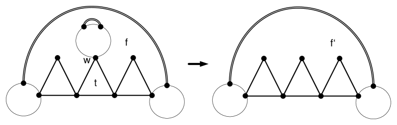
Figure 18: Contraction operation when contains a trapped triangle’s free side. -
•
Now we prove the second property. Let and be an adjacent pair of triangles whose free sides bound the super-face . We will argue that and are strongly adjacent, with being the free vertex of and being the common vertex. Assume that they were not strongly adjacent.
Notice that, since the free sides for both bound a common super-face , this can only happen if has a connected component drawn inside (see Figure 19.)
Observe that contains only heavy cactus triangles: Any type- or type- edge with exactly one end point in can only be incident on and must be drawn in the exterior of . Again, as in the previous case, we can do the contraction trick to argue that there exist two type- or type- edges and bounding face such that and they are not adjacent.
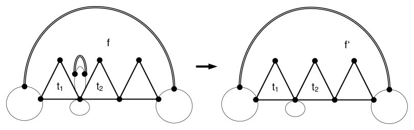
Figure 19: Contraction operation when contains a pair of free sides which corresponds to a pair of weakly-adjacent triangles.
∎
5.5 Proof of the Friend Lemma (Proof of Lemma 5.2)
In this section, we prove the friend lemma. We will rely on some structural observations:
Lemma 5.13
Let and be any heavy cactus triangle such that , and be its (unique) cactus edge for which . Then, we have .
Proof.
Let be a maximal trail along the boundary of starting from and only visiting vertices in in graph . Notice that may use cactus edges or type- or type- edges. Let be the other endpoint of and be the next edge on the boundary of , such that . First, notice that cannot be in , for otherwise, we would have the free sides of on different super-faces. Therefore, . Now, let be a maximal trail from along the boundary of , visiting only vertices in . We claim that must contain : Otherwise, let be the last node on and be the next edge on incident to . Consider a region bounded by (i) the sides of on super-face ,(ii) trail ,and (iii) any path from to using only cactus edges in . This close region must contain super-face , so must be drawn inside (see Figure 20). This is a contradiction since cannot connect to a node in (same reasoning as before), and similarly it cannot connect to (this would contradict the choice of or the edge .). ∎
Observation 5.14
For any heavy triangle , the free or base sides will be adjacent to two different super-faces in .
Lemma 5.15
Let be a heavy triangle. Let be the two different super-faces that contain the base and free sides of respectively. Let be the unique type- or type- edges on and across the occupied components of (given by Lemma 5.13). Then .
Proof.
Assume otherwise that , so the super-faces and are adjacent at . This means that there is only one type- or type- edge across the occupied components, contradicting to the fact that is heavy (see Fig. 21 for illustration). ∎
Components for two adjacent heavy triangles:
Now we fix the labelling for the new components created by the operation of removing edges for two adjacent heavy triangles from , which we will use in the rest of this section. Every time when we talk about two adjacent heavy triangles we will denote them by such that and , where will be the corresponding free vertices and the common base vertex of and . The vertices of the new components formed by removing edges from will be , such that and . Notice that the free components of are respectively, the occupied components of are and the occupied components of are .
Lemma 5.16
Let be a super-face. Let be two adjacent heavy cactus triangles with (say ) such that for . For each , let be the base edge and (unique due to lemma 5.13).
-
1.
if and only if the common edge goes across and .
-
2.
if and only if both are incident to .
Proof.
The first direction for item 1 is easy to see by the way are defined and by the fact that goes across the occupied components for both . In the other direction, if goes across , hence it also goes across the occupied components for . This along with the fact that belongs to and Lemma 5.13, it implies that .
Lemma 5.17
Let be a super-face. Let be two adjacent heavy cactus triangles with (say ) such that both of whose free sides belong to . If the base sides for and belong to two different super-faces and for each , let (unique due to lemma 5.15). Then at least one of or is incident on some vertex in , which in turn implies .
Proof.
As are adjacent, we use the notations defined above for the various components corresponding to two adjacent heavy triangles. First, assuming that at least one of or is incident on some vertex in , we prove that .
By contradiction, let . Now we show that there will be a cycle in sharing an edge with , contradicting the fact that is a triangular cactus (see Figure 23). By the above claim, this edge is incident to (say ). Also, by the way and are defined, the other end point belongs to both and . Hence in , using only cactus edge, there is a path from to and another path from to . Hence, is a cycle in sharing edge with , contradicting the fact that is a triangular cactus.
Finally, to finish the proof for our lemma, we prove that at least one of or is incident on some vertex in .
For contradiction assume none of are incident on . Notice that since free sides of belongs to the same super-face , we can partition the component into two parts (with an exception that is a common vertex), such that is drawn inside , outside of and lies on .
Starting with vertex and the base side create a maximal trail in along the boundary of by visiting type- or type- or cactus edges and vertices only from . This trail should end at some vertex (possibly ), such that there is a type- or type- edge leaving incident on (say ). If not, then the trail would end at and the base side will be the next edge belonging to super-face in the graph , which contradicts our assumption. Notice that since are the free components, hence either or . In case when , it implies that is an edge going across the components of and also belongs to . But by Lemma 5.13, it implies that , contradicting our assumption (see Figure 24).
In the other case, when , we look at the original graph . Since both , there exists a path from to using only cactus edges and vertices from . Similarly since , there exists a path from to using only cactus edges and vertices from . Hence, the region bounded by contains only the vertices from at its boundary and also contains the base edge from the side outside of . This implies that the super-face can only be drawn inside and can only contain vertices from and hence for to go across the occupied components of , the only possibility is to go across and , contradicting our assumption (see Figure 24).
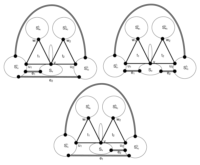
∎
Proof of the first part
We assume that for contradiction that are friends where is type- triangle. We will argue that there exists an improving -swap, contradicting the fact that is the optimal cactus. As are adjacent, we use the notations defined above for the various components corresponding to two adjacent heavy triangles.
Let be the supported cross triangle of and let be the empty triangle formed by vertices . Also let (possibly same) be the type- or type- edges belonging to the super-face going across the occupied components of respectively (exists by Lemma 5.13). Also, let be the edge going across the occupied components of which belongs to the super-face containing the base side for (exists by Lemma 5.13). By Lemma 5.15, .
Now there could be two cases based on the landing components for supported cross triangles . The second case will be further divided into sub-cases based on the way is drawn in .
-
•
( is a type- edge and different landing components for supported cross triangles ): We modify our cactus by (see Figure 25). Note that will attach to , will attach with and and finally will attach to this structure, hence will be a triangular cactus with one more cactus triangle, which contradicts the optimality of .
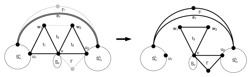
Figure 25: Improving -swap when the edge given by Lemma 5.13 is type- and the cross triangles supported by and have different landing components. -
•
( is a type- edge and share a common landing component): Since is the unique edge belonging to going across the occupied components of (see Lemma 5.13), there could be two sub-cases.
-
–
( goes across ): From Lemma 5.16 it implies that . Now if we focus on , the base side of it must belong to a super-face such that goes across its occupied components such that and (by Observation 5.14, Lemma 5.13 and 5.15). Also, by the uniqueness of the edge , the edge cannot belong to . But this implies that is drawn inside and is drawn outside it, hence by Observation 3.2 cannot share their landing components, contradiction.
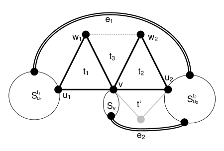
Figure 26: The case when the edge given by Lemma 5.13 is type- and the cross triangles supported by and have the same landing component. If goes across , then due to the presence of , the landing component for cannot be the same. -
–
( goes across ): By Lemma 5.16, it implies and both are incident on . Now let such that and . Since both , there exists a path from to using only cactus edges and vertices from . Similarly since , there exists a path from to using only cactus edges and vertices from . Hence, the region bounded by contains only the vertices from at its boundary and also contains the base edge (see Fig. 27). This implies that the super-face can only be drawn inside and consecutively the triangle is drawn inside . This implies that should be drawn outside and consecutively is drawn outside , hence by Observation 3.2 cannot share their landing components, contradiction.
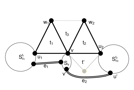
Figure 27: The setting before we reach a contradiction for the case when the edge given by Lemma 5.13 is type- and the cross triangles supported by and have the same landing component. If goes across , then will go across , hence the landing component for cannot be the same.
-
–
Second part
For contradiction we assume that are friends. Again are adjacent, hence we use the notations defined above for the various components corresponding to two adjacent heavy triangles. Let be the triangle formed by vertices . Also let be the unique type- or type- edge belonging to the super-face containing base side of going across occupied components of (exists by Lemma 5.13) and be the unique type- or type- edge belonging to the super-face containing base side of going across occupied components of (exists by Lemma 5.13). Let (possibly same) be the unique type- or type- edges belonging to the super-face going across occupied components of respectively (exists by Lemma 5.13 and the fact that contains free sides for both .). By Lemma 5.15 and 5.17, , and .
Now we fix the cross triangles each supported by respectively, as follows. The idea here is to fix these supported cross triangles in such a way that their landing components are as different as possible. If supports a cross triangle drawn inside , then we fix to be that triangle, otherwise is any supported cross triangle of . If there exists a cross triangle supported by which does not share its landing component with then we fix to be that triangle, otherwise is any supported cross triangle of . Similarly, we choose the supported cross triangle of such that it does not share its landing component with any of or (or both), otherwise is any supported cross triangle of .
By the way are chosen, it ensures that all three of them can share a landing component if and only if all three are type- edges (by Lemma A.1). Now there could be three cases.
-
•
( have different landing components): Since the base sides for are in different super-faces, Lemma 5.17) implies that at least one of is incident on (by renaming assume ). Hence, if the triangles do not share their landing components then we modify our cactus by (See Figure 28). Note that will attach to , will attach with and and finally will attach to this structure, hence will be a triangular cactus with one more cactus triangle, which contradicts the optimality of .
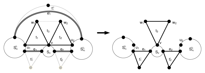
Figure 28: Improving -swap when there exist two cross triangles supported by respectively such that their landing components are different. -
•
( has a different landing component than the common landing component for ): In this case we know that share their landing components but the landing component for is different. Again, since the base sides for are in different super-faces, Lemma 5.17) implies that at least one of is incident on . Now there are two sub-cases:
-
–
( incident on ): In this case, we modify our cactus by (See Figure 29). Again will attach with , will attach with and and finally will attach to this structure, hence will be a triangular cactus with one more cactus triangle, which contradicts the optimality of .
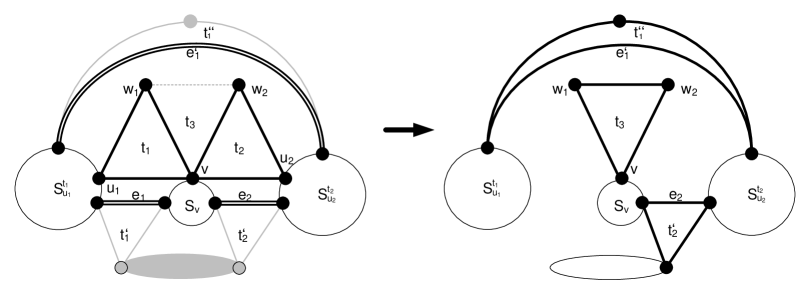
Figure 29: Improving -swap when there exists two cross triangles supported by respectively such that their landing components are different. -
–
(Only incident on ): In this case goes across .
-
*
( incident on ): The modification gives us the contradiction since will attach to , will attach with and and finally will attach to this structure, hence will be a triangular cactus with one more cactus triangle, which contradicts the optimality of .
-
*
( goes across ): The modification (See Figure 30) gives us the contradiction since will attach to , will attach with and and finally will attach to this structure, hence will be a triangular cactus with one more cactus triangle, which contradicts the optimality of .
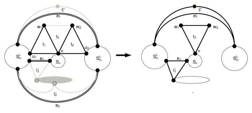
Figure 30: Improving -swap when there exists two cross triangles supported by respectively such that their landing components are different.
-
*
-
–
-
•
(All three triangles share their landing components): In this case, all three are type- edges. Also by Lemma 5.17, at least one of will be incident on . And since are free components, none of the three edges can be incident on . Based on these facts, there could be two sub-cases:
-
–
(Exactly one of or is incident on ): We will argue that this case cannot occur, by showing that there is no way for to share the same landing component with . Since are friends, all the vertices of (except ) are drawn outside . This also implies that there is a trail starting from vertex , using all the cactus/type-/type- edges on the outer-face for and finally reaching , such that the only repeated vertex in the trail is . Since exactly one of or is incident on , this implies that the other one goes across (say ) such that and . This means that there exists a circuit comprising of only cactus/type-/type- edges formed by concatenating the trail , the path between and using cactus edges/vertices only from , the path between and using cactus edges/vertices only from and the type- or type- edge . It is easy to see that this circuit partitions the plane into two regions, say , such that all the vertices of are drawn inside as a hole and the free sides for are drawn in such that the only vertex from on the boundary for these regions is . Also, the presence of the edge does not allow the vertex to be a part of any type- or type- edge drawn inside . This implies that the edge out of which is incident on will be drawn inside and will be drawn outside , which contradicts the fact that all three supported cross triangles share their landing component.
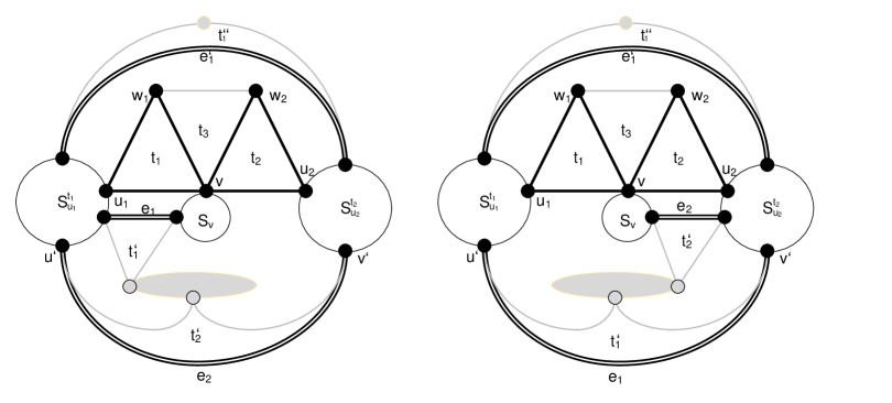
Figure 31: The setting before we reach a contradiction in the case where all three edges are type- and the landing component for the respective supported cross triangles is the same. Also, exactly one of or is incident on . This case cannot occur since then cannot reach the landing component of . -
–
(Both and are incident on ): Now we focus on , which is a heavy type- triangle and look at the type- or type- edges going across ’s occupied components. The two type- edges and are surely going across the occupied components of . By Prop. 2.4, should have at least one more such type- or type- edge (say ). Now let and . This means that there is a path from to in and another path from to in such that the cycle is made of only cactus/type-/type- edges and cactus vertices such that it divided the plane into two regions such that one region contains the base side of and another contains the free side for . Since, see the base and free sides for respectively, hence they have to be drawn in the different region bounded by . Hence, the cross triangles supported by cannot share their landing components, contradiction.
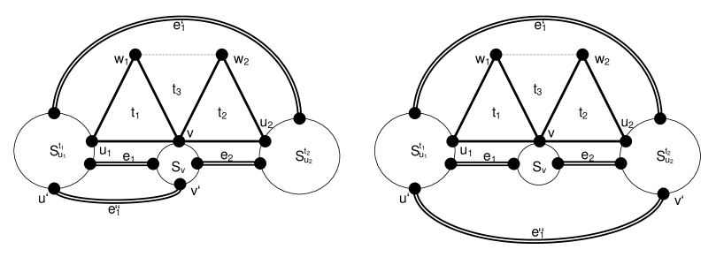
Figure 32: The setting before we reach a contradiction in the case where the edges are type- and the landing component for the respective supported cross triangles is the same. Also, both and are incident on . This case cannot occur since is a type- heavy triangle and the additional type- or type- edge going across ’s occupied components will separate into different regions.
-
–
6 On the Strength of Our Result
6.1 Our Bound is Almost Tight
In this section, we show that there exists a graph for which . We show this indirectly using a family of graphs presented in [7], as stated in the following lemma.
Lemma 6.1
[7] There is a family of -vertex planar graphs for which there exist a maximal cactus subgraph of such that .
In [7], this family of graphs is used to show that a maximal cactus (not maximum) is not sufficient to improve over the best known greedy strategies when approximating MPT. In the context of this paper we use to compare it to a maximum cactus for to prove the following.
Theorem 6.2
Let be the graph family as in Lemma 6.1. Then, .
Proof.
By Lemma 6.1, it suffices to argue that . Let be an optimal cactus with triangles. Notice that for any triangle in , intersects at most two other triangles in . If all three edges of were to be used by three different triangles in , this would contradict the cactus property. Moreover, if does not intersect any triangle in this would imply that one of its edges would complete a cycle if added to . By these two observations we can use a simple counting scheme to upper-bound the number of triangles in depending on the number of triangles in . We iteratively add triangles of to and count in every step how many triangles in need to be removed to maintain the cactus property. For every triangle in that intersects in one or two edges, we have to remove at most two triangles from . For every triangle in , that does not intersect in any edge, we have to break a cycle in the resulting by deleting one other triangle from it. In each iteration we therefore destroy at most two triangles from the original and therefore get . This concludes the proof as . ∎
6.2 Comparison to the Previous Bound
One integral part to derive the improved approximation ration for MPS in [3] was to show that for any given planar graph with vertices and edges, we have:
Theorem 6.3 ([3])
Let be as above, then .
As removing one edge from a triangulated planar graph merges exactly two faces, we can easily derive a lower bound that depends on , for the number of triangular faces in :
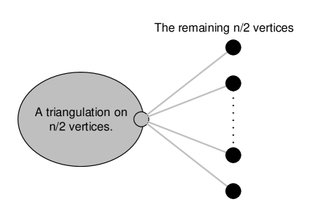
We end this section by showing that the bound in [3] alone is not sufficient for approximating MPT. To this end we construct a graph in which , even though , Let be a planar graph with vertices, where vertices form a triangulated planar subgraph. Let be a vertex on the outer-face of this triangulated structure. The remaining vertices are embedded in the outer-face and are incident to exactly one edge each, with the other endpoint being (see Figure 33 for an illustration of this construction). Therefore by Euler’s formula, the number of edges in this graph is equal to and thus , while the number of triangular faces is .
7 Conclusions and Open Problems
Our work implies that a natural local search algorithm gives a -approximation for MPS and a approximation for MPT. To be more precise, when given any graph , we follow the -swap local search strategy for : Start from any cactus subgraph . Try to improve it by removing triangles and adding triangles in a way that ensures that the graph remains a cactus subgraph. A local optimal solution will always be a approximation for MPS and a approximation for MPT.
Knowing this fact, there is an obvious candidate algorithm for improving over the long-standing best approximation factor for MPS. We call a graph a diamond-cactus if every block in is either a diamond888A diamond subgraph is a graph that is isomorphic to the graph resulting from deleting any single edge from a . or a triangle. Start from any diamond-cactus subgraph of and then try to improve it by removing triangles from and adding triangles, maintaining the fact that is a diamond-cactus subgraph. We conjectured that this algorithm gives a better than -approximation for MPS, but we suspect that the analysis will require substantially new ideas.
Another interesting direction is to see whether there is a general principle that captures a denser planar structure than cactus subgraphs by going above matroid parity in the hierarchy of efficiently computable problems. For instance, are diamond-cactus subgraphs captured by matroid parity? Or can it be formulated as an even more abstract structure than matroids (e.g. commutative rank [2]) that can still be computed efficiently? We believe that studying this direction will lead to a better understanding of algebraic techniques for finding dense planar structures.
Finally, the absence of LP-based techniques in this problem domain seems rather unfortunate. There have been some experimental studies recently, but the theoretical understanding of what can be proven formally in the context of power of relaxation is certainly lacking [16, 10, 11]. Is there a convex relaxation that allows us to find a relatively dense planar subgraph (e.g. -approximation for MPS using LP-based techniques)?
Acknowledgement:
Parinya Chalermsook is supported by the European Research Council (ERC) under the European Union’s Horizon 2020 research and innovation programme (grant agreement No 759557) and by Academy of Finland Research Fellows, under grant number 310415 and 314284. Sumedha Uniyal is partially supported by Academy of Finland under the grant agreement number 314284.
References
- [1] Claude Berge. La theorie des graphes. Paris, France, 1958.
- [2] Markus Bläser, Gorav Jindal, and Anurag Pandey. Greedy strikes again: A deterministic PTAS for commutative rank of matrix spaces. In 32nd Computational Complexity Conference, CCC 2017, July 6-9, 2017, Riga, Latvia, pages 33:1–33:16, 2017.
- [3] Gruia Călinescu, Cristina G Fernandes, Ulrich Finkler, and Howard Karloff. A better approximation algorithm for finding planar subgraphs. Journal of Algorithms, 27(2):269–302, 1998.
- [4] Gruia Calinescu, Cristina G Fernandes, Howard Karloff, and Alexander Zelikovsky. A new approximation algorithm for finding heavy planar subgraphs. Algorithmica, 36(2):179–205, 2003.
- [5] Gruia Călinescu, Cristina G Fernandes, Hemanshu Kaul, and Alexander Zelikovsky. Maximum series-parallel subgraph. Algorithmica, 63(1-2):137–157, 2012.
- [6] Parinya Chalermsook, Marek Cygan, Guy Kortsarz, Bundit Laekhanukit, Pasin Manurangsi, Danupon Nanongkai, and Luca Trevisan. From gap-eth to fpt-inapproximability: Clique, dominating set, and more. In Foundations of Computer Science (FOCS), 2017 IEEE 58th Annual Symposium on, pages 743–754. IEEE, 2017.
- [7] Parinya Chalermsook and Andreas Schmid. Finding triangles for maximum planar subgraphs. In WALCOM: Algorithms and Computation, 11th International Conference and Workshops, (WALCOM’17), Proceedings., pages 373–384, 2017.
- [8] Parinya Chalermsook, Andreas Schmid, and Sumedha Uniyal. A Tight Extremal Bound on the Lovász Cactus Number in Planar Graphs. In 36th International Symposium on Theoretical Aspects of Computer Science (STACS 2019), volume 126 of Leibniz International Proceedings in Informatics (LIPIcs), pages 19:1–19:14. Schloss Dagstuhl–Leibniz-Zentrum fuer Informatik, 2019.
- [9] Ho Yee Cheung, Lap Chi Lau, and Kai Man Leung. Algebraic algorithms for linear matroid parity problems. ACM Transactions on Algorithms (TALG), 10(3):10, 2014.
- [10] Markus Chimani, Ivo Hedtke, and Tilo Wiedera. Exact algorithms for the maximum planar subgraph problem: New models and experiments. In 17th International Symposium on Experimental Algorithms, SEA 2018, June 27-29, 2018, L’Aquila, Italy, pages 22:1–22:15, 2018.
- [11] Markus Chimani and Tilo Wiedera. Cycles to the Rescue! Novel Constraints to Compute Maximum Planar Subgraphs Fast. In Yossi Azar, Hannah Bast, and Grzegorz Herman, editors, 26th Annual European Symposium on Algorithms (ESA 2018), volume 112 of Leibniz International Proceedings in Informatics (LIPIcs), pages 19:1–19:14, Dagstuhl, Germany, 2018. Schloss Dagstuhl–Leibniz-Zentrum fuer Informatik.
- [12] Harold N Gabow and Matthias Stallmann. An augmenting path algorithm for linear matroid parity. Combinatorica, 6(2):123–150, 1986.
- [13] Magnús M Halldórsson. Approximations of weighted independent set and hereditary subset problems. In Graph Algorithms And Applications 2, pages 3–18. World Scientific, 2004.
- [14] Johan Håstad. Clique is hard to approximate withinn 1- . Acta Mathematica, 182(1):105–142, 1999.
- [15] T.A. Jenkyns. Matchoids : a Generalization of Matchings and Matroids. Thesis (Ph.D.)–University of Waterloo, 1974.
- [16] M. Jünger and P. Mutzel. Maximum planar subgraphs and nice embeddings: Practical layout tools. Algorithmica, 16(1):33–59, Jul 1996.
- [17] Subhash Khot and Ashok Kumar Ponnuswami. Better inapproximability results for maxclique, chromatic number and min-3lin-deletion. In International Colloquium on Automata, Languages, and Programming, pages 226–237. Springer, 2006.
- [18] Eugene L Lawler. Combinatorial optimization: networks and matroids. Courier Corporation, 1976.
- [19] Jon Lee, Maxim Sviridenko, and Jan Vondrák. Matroid matching: the power of local search. SIAM Journal on Computing, 42(1):357–379, 2013.
- [20] John M Lewis and Mihalis Yannakakis. The node-deletion problem for hereditary properties is np-complete. Journal of Computer and System Sciences, 20(2):219–230, 1980.
- [21] László Lovász. Matroid matching and some applications. Journal of Combinatorial Theory, Series B, 28(2):208–236, 1980.
- [22] László Lovász and Michael D Plummer. Matching theory, volume 367. American Mathematical Soc., 2009.
- [23] Carsten Lund and Mihalis Yannakakis. The approximation of maximum subgraph problems. In International Colloquium on Automata, Languages, and Programming, pages 40–51. Springer, 1993.
- [24] James B Orlin. A fast, simpler algorithm for the matroid parity problem. In International Conference on Integer Programming and Combinatorial Optimization, pages 240–258. Springer, 2008.
- [25] Zoltán Szigeti. On a min-max theorem of cacti. In International Conference on Integer Programming and Combinatorial Optimization, pages 84–95. Springer, 1998.
- [26] William T Tutte. The factorization of linear graphs. Journal of the London Mathematical Society, 1(2):107–111, 1947.
Appendix A Missing Proofs
A.1 Proof of Proposition 2.4
Observation 3.2 immediately leads to a simple lemma which will prove helpful in the proof of Proposition 2.4.
Lemma A.1
Let be a type- edge in , then the cross triangles and supported by can not have the same landing component.
Proof.
Since both and are in , there exists a path from to in containing only cactus edges and vertices (see for example Figure 3). Hence, the cycle consists of only type- or type- or cactus edges and cactus vertices, such that the two cross triangles supported by will be drawn in different regions corresponding to . Thus by Observation 3.2 the two cross triangles supported by cannot have the same landing component. ∎
The -swap introduced in Figure 2(a) and the -swap optimality of , implies the following lemma.
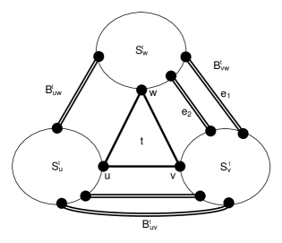
Lemma A.2
Let be a cactus triangle with vertices and and let there exist at least two cross triangles in such that , for , then
-
i
and must have the same landing component,
-
ii
any edge in is of type-,
-
iii
and
-
iv
any set of edges for support at most one cross triangle.
Proof.
To prove property (i), assume for contradiction that and do not share the same landing component. In this case we can increase the number of triangles in by removing from and adding and to in its place. As the landing components are disjoint this operation does not introduce any new cycle to other than the supported cross triangles and therefore the resulting structure is a cactus subgraph of . This contradicts that is -swap optimal.
Property (ii) follows from property (i). Assume for contradiction that there exists a type- edge (the same argument will hold for and ). Only one of and can have its two cactus vertices in the same split components of as the endpoints of . We may assume that this is not the case for . Let and denote the cross triangles supported by . By property (i) and must have the same landing component, the same holds for and . But by Lemma A.1 and can not have the same landing component, thus we reach a contradiction.
We will prove property (iii) also by contradiction. Assume that and let be any two type- edges (the same argument will hold for and ). As both endpoints of are cactus vertices, there exists a path in connecting both the endpoints, thus there is a cycle in containing and only cactus edges otherwise. Similarly, there exists a cycle in that contains and only cactus edges otherwise. In either is embedded in the inside of the closed region bounded by or is embedded in the inside of the closed region bounded by (see Figure 34). We may assume the former case as the proof for the later case is symmetric.
Only one of and can have its two cactus vertices in the same split components of as the endpoints of . We may assume that this is not the case for . By property (i) the cross triangle supported by and must have the same landing component. Note can not lay in the inside of the region bounded by in . Therefore the landing component shared by the two cross triangles must lie on the outside of . However, by property (i) the cross triangle supported by and must have the same landing component. We reach a contradiction using Obs. 3.2.
We prove property (iv) also by contradiction. Assume that the set of edges supports two cross triangles (the same argument will hold for and ). Property (iii) implies that there is only one type- edge in hence will support the other cross triangle. Let be the triangles supported by , be the cross triangle supported by an edge . Only one of and can have its two cactus vertices in the same split components of as the endpoints of . We may assume that this is not the case for . By property (i), and must have the same landing component. But this is also true for and . In addition there is a cycle in that contains and a path from to in (where ) containing only cactus vertices and edges such that is embedded in its inside in and outside of it. As intersects it must be drawn outside of in . But by Observation 3.2, and cannot have the same landing component and we reach a contradiction. ∎
Further we can show that
Lemma A.3
If supports cross triangles and , where denotes their common cactus vertex, then and are both empty.
Proof.
By Lemma A.2, item (i), and must have the same landing component. Note that if and have a common landing vertex, then the claim is trivially true, as then is incident to exactly three faces, namely , and which by definition are all empty and thus and are empty in this case. Thus we assume that .
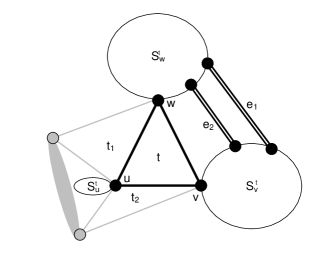
Let and denote the landing vertices of and respectively. As and have the same landing component (say ), must contain a path from to consisting of edges only in . Furthermore forms a cycle with only one cactus vertex and cross edges and edges in . Note that the fact that and are empty in , implies that the two cactus edges of incident to , as well as the edges and are consecutive in the circular edge incident list of in . This observation gives us two important facts. First, as contains and , any other edge incident to in must be drawn in the region bounded inside of in . Second, any split component , for , must be drawn outside of in . Assume for contradiction that there exists an edge with endpoints and , with , by the previous observation has to cross in and therefore the existence of contradicts that is a plane graph. Similarly, there cannot exist any edge with one endpoint in and another endpoint in , with , since all these vertices are drawn strictly inside of and ’s, with , are drawn strictly outside of . ∎
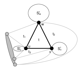
We are now ready to prove the different properties of heavy triangles claimed in Proposition 2.4. In the following we will prove one lemma for every such claim.
Lemma A.4
Any cactus type- triangle in is light.
Proof.
For any vertex in , there is a pair of cross triangles supported by such that their intersection is , thus by Lemma A.3, must be empty for any . Hence the number of cross triangles supported by and is less than four and each edge supports one cross triangle, thus is a light triangle. ∎
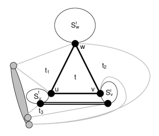
Lemma A.5
Any cactus type- triangle in is light.
Proof.
Let be a type- triangle, such that each of the cactus edges and support a cross triangle respectively (see Figure 37). By Lemma A.3, and must be empty. By Lemma A.2 properties (ii) and (iii) there is at most one edge in and if it exists it must be of type-. Thus there are at most three cross triangles supported by and the edge in and in addition at least two edges in support a cross triangle, thus is a light triangle. ∎
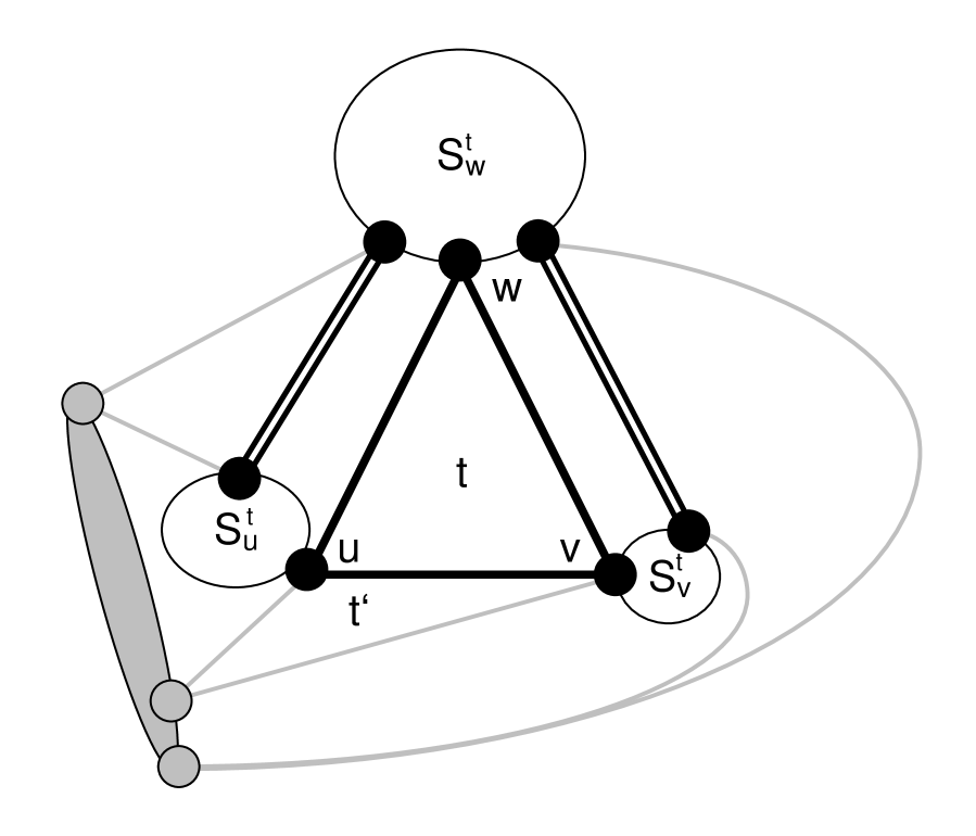
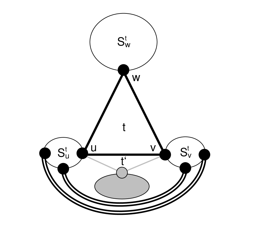
Lemma A.6
If is a heavy type- triangle, with , let denote the edge in that supports the cross triangle supported by , then for all and the total number of cross triangles supported by edges in is greater than or equal to two.
Proof.
We first show that is empty for every . Let denote the cross triangle supported by . Assume for contradiction, that there exists an edge in some for some edge . As and the cross triangle supported by fulfill the requirements of Lemma A.2, property (iv) implies that there are at most three cross triangles supported by edges in , which contradicts the definition of a heavy triangle.
As and are empty there must be at least two cross triangles in supported by edges in , as otherwise would be light. ∎
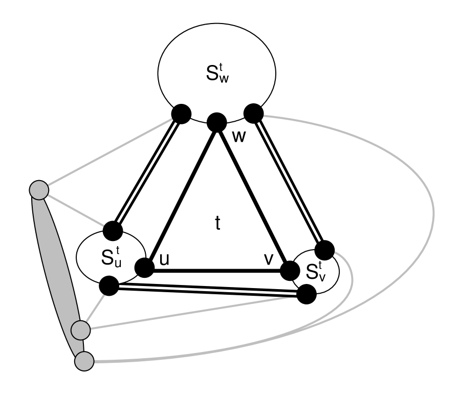
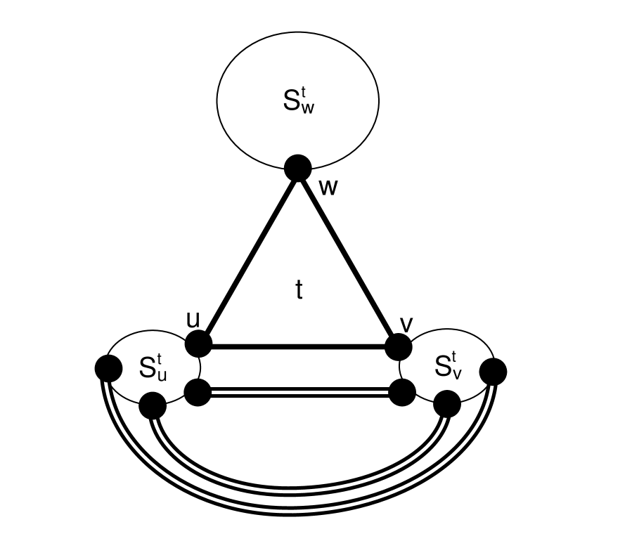
Lemma A.7
If is a heavy type- triangle, then there is an edge such that for all and the total number of cross triangles supported by edges in is greater than or equal to three.
Proof.
We will first show that at most one of for can be non-empty. Assume for contradictions that there are two sets and which are non-empty. Then the cross triangles supported by the edges in these two sets fulfill the requirements of Lemma A.2. Hence and the number of cross triangles supported by is at most three, contradicting the fact that is heavy.
Therefore we know that there is only one edge such that is non-empty. As is heavy must contain edges which support at least three cross triangles as otherwise would be light. ∎
A.2 Proof of Proposition 3.1
In this section we will prove the properties stated in Proposition 3.1 about light triangles. Recall that for a light triangle the edges in support at most three cross triangles.
Lemma A.8
If is a light type- triangle with one edge such that for all , then the total number of cross triangles supported by edges in is at most two.
Proof.
This simply follows from the definition of heavy triangles. If there where more than two cross triangle supported by the edges in , then would be a heavy triangle. ∎
Lemma A.9
If is a light type- triangle where supports the cross triangle supported by and for all , then the total number of cross triangles supported by edges in is at most one.
Proof.
This simply follows from the definition of heavy triangles. If there was more than one cross triangle supported by the edges in , then would be a heavy triangle. ∎
Lemma A.10
If is a light triangle where the edges in support either two or three cross triangles such that at least two different sets of edges for support a cross triangle each, then each set of edges supports at most one cross triangle and all the supported cross triangles have the same landing component.
A.3 Proof of Lemma 5.8
Below, we analyze the contribution from non outer-faces.
| Coordinates | Value |
|---|---|
This is simply an algebraic manipulation. First, we write
We will gradually decompose the vector
into several meaningful terms that we could upper bound. First, we focus on the coordinates that correspond to the (highlighted in blue):
where we simply applied the fact that . Next, we focus on the components of and (shown in red).
where we applied the upper bound from Lemma 5.7 (first bound). We further extract the “components” of , and :
the inequality was obtained by applying Lemma 5.7 (second bound). Now, we extract the components of , and (the 3rd, 6th, and 9th coordinates respectively.)
here we applied the third bound of Lemma 5.7, and the fact that all coordinates of vector are non-negative. Finally, by summing over all terms in the boxes, we get the upper bound of
Now, since and , we have that
Hence, .
Appendix B Tight Examples
B.1 Tight Example of Factor for a -swap Optimal Solution
Following is the family of tight examples for the factor analysis. In these examples, for some , , , , , , , , , and all other . Notice that each inequity which we use in the above proof is asymptotically tight for these example.

B.2 Tight Example of Factor for a -swap Optimal Solution
Following is the family of tight examples for the factor analysis. In these examples, for some , , , , , , , , , and all other . Notice that each inequity which we use in the above proof is asymptotically tight for these example.
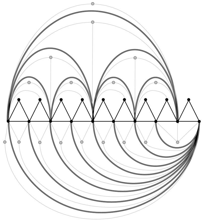
Appendix C Definition of Variables
| Variable | Description |
|---|---|
| initial plane graph with a fixed drawing | |
| optimal triangular cactus which is a subgraph of | |
| a connected component of cactus | |
| # triangular faces in the cactus | |
| # triangular faces of with at least two vertices in | |
| type- edges supporting no triangles | |
| type- edges supporting triangle | |
| type- edges supporting triangles | |
| type- triangles supporting no triangles | |
| type- triangles supporting triangle | |
| type- triangles supporting triangles | |
| type- triangles supporting triangles | |
| subgraph of after removing type- edges | |
| The new components in , such that for every | |
| = for every | |
| type- or type- edge with one end-point each in | |
| set of super-faces in excluding the cactus triangular faces of | |
| # of supporting side of type- edges in | |
| # of non-supporting side of type- edges in | |
| # of type- edges in | |
| # of base edges of type- triangles in | |
| # of free pair of edges of type- triangles in | |
| # of base edges of type- triangles in | |
| # of free pair of edges of type- triangles in | |
| (length of face ) | |
| (occupied length of face ) | |
| (free length of face ) | |
| # surviving faces in some | |
| length of outer-super-face of graph | |
| # of , and side edges in outer-face of graph | |
| Outer-face of graph | |
| set of super-faces of type- such that for any , | |
| , and . | |