Evolving Black Holes in Inflation

Abstract

We present an analytic, perturbative solution to the Einstein equations with a scalar field that describes dynamical black holes in a slow-roll inflationary cosmology. We show that the metric evolves quasi-statically through a sequence of Schwarzschild-de Sitter like metrics with time dependent cosmological constant and mass parameters, such that the cosmological constant is instantaneously equal to the value of the scalar potential. The areas of the black hole and cosmological horizons each increase in time as the effective cosmological constant decreases, and the fractional area increase is proportional to the fractional change of the cosmological constant, times a geometrical factor. For black holes ranging in size from much smaller than to comparable to the cosmological horizon, the pre-factor varies from very small to order one. The “mass first law” and the “Schwarzchild-de Sitter patch first law” of thermodynamics are satisfied throughout the evolution.

I Introduction

The dynamics of black holes in cosmology is important for understanding several questions about the very early universe. During very hot phases a population of black holes will affect the behavior of the plasma and impact upon phase transitions, and could even have a significant effect on the the geometry near the big-bang. On the late time, or ‘cooler’ side, there has been interesting recent research Bird:2016dcv ; Sasaki:2016jop ; Carr:2016drx ; Sasaki:2018dmp about the possibility of an early population of black holes that could seed galaxies and provide progenitors for the larger black holes detected by LIGO Abbott:2016blz ; TheLIGOScientific:2016htt .

Such situations are highly interactive involving classical accretion, the expansion of the universe, as well as classical and quantum mechanical radiation exchange. Known analytic solutions include the stationary Kerr-Reissner-Nordstrom de Sitter metric Carter:1973rla , the cosmological McVittie black hole spacetime McVittie:1933zz , which has an unphysical pressure field except when it reduces to Schwarzschild-de Sitter Kaloper:2010ec , and cases of multi, maximally charged, black holes Kastor:1992nn ; Horne:1993sy ; Gibbons:2009dr ; Maeda:2010aj that exploit fake supersymmetries Chimento:2012mg ; Klemm:2015qpi . A range of approximations and numerical analyses have been used to study accretion and estimate the growth of black holes in these interactive systems, including Frolov:2002va ; Jacobson:1999vr ; Saida:2000at ; Harada:2004pf ; Sultana:2005tp ; MartinMoruno:2006mi ; JimenezMadrid:2005rk ; MartinMoruno:2008vy ; Faraoni:2007es ; Carrera:2008pi ; Rodrigues:2009eg ; Carr:2010wk ; UrenaLopez:2011fd ; Guariento:2012ri ; Rodrigues:2012xm ; Chadburn:2013mta ; Abdalla:2013ara ; Babichev:2005py ; Babichev:2008jb ; Babichev:2012sg ; Babichev:2014lda ; Davis:2014tea ; Afshordi:2014qaa ; Davis:2016avf . Many of these studies incorporate test stress-energy and infer time rate of change of the black hole mass by computing the flux of stress-energy across the horizon. In this paper we continue our studies of the evolution of black holes in inflationary cosmologies by solving the full coupled scalar field plus Einstein equations in the slow-roll and perturbative approximations. This system has the advantage that it is only “mildly dynamical”, and quantities can be computed in controlled approximations. While mild, we anticipate that the solution presented here will be useful for computing observational signals of black holes that are present during the inflationary epoch, and helpful in developing techniques applicable to hotter early universe situations.

Slow-roll inflationary cosmologies are described by quasi-de Sitter metrics, in which the cosmological constant, $\Lambda$, is provided by the potential of a scalar field $\phi$, and $\Lambda$ slowly evolves in time as $\phi$ rolls down a potential. If a black hole is included, one thinks about the spacetime as being approximately described by quasi-Schwarzschild-de Sitter metrics, with both $\Lambda$ and the mass parameter $M$ changing slowly. But is this picture correct? Here we answer this question in the affirmative. We show that the black hole plus scalar field system evolves through a sequence of very nearly Schwarzschild-de Sitter (SdS) metrics as the inflaton rolls down the potential.

In earlier work, Chadburn and Gregory Chadburn:2013mta found perturbative solutions for the black hole and scalar field cosmology, as the field evolves slowly in an exponential potential. Their null-coordinate techniques were particularly useful for analyzing the behavior of the horizon, and computing the growth of the horizon areas. Recently we extended the work of Chadburn:2013mta to general potentials Gregory:2017sor , with a focus on evolutions that interpolate between an initial SdS and final SdS with a smaller cosmological constant $\Lambda$. The analysis yielded geometrical expressions for the total change in the horizon areas. Further, it was found that the “SdS-patch” first law was obeyed between the initial and final SdS states. The SdS-patch first law Dolan:2013ft only involves quantities defined in the portion of the spacetime between the black hole and cosmological horizons, see equation (9) below. That result supports the picture of a quasi-static evolution through SdS metrics, which we address in detail in this paper.

Consider Einstein gravity coupled to a scalar field with potential $W(\phi)$ governed by the action

$$S=\int d^{4}x\sqrt{-g}\left(\frac{M_{p}^{2}}{2}R-(\nabla\phi)^{2}-2W(\phi)\right)$$ (1)

where $M_{p}^{2}=1/8\pi G$ is the reduced Planck Mass in units with $\hbar=c=1$. Varying the action yields Einstein’s equation $G_{ab}=T_{ab}/M_{p}^{2}$ with the stress-energy tensor given by

$$T_{ab}=\nabla_{a}\phi\nabla_{b}\phi-\frac{1}{2}g_{ab}\left[(\nabla\phi)^{2}+2W(\phi)\right]$$ (2)

and the scalar field equation of motion is given by

$$g^{ab}\nabla_{a}\nabla_{b}\phi=\frac{\partial W}{\partial\phi}\,.$$ (3)

The coordinate system used in Gregory:2017sor was chosen to facilitate analysis of the horizons and clarify the degrees of freedom of the metric, but did not prove amenable for finding the full time-dependent corrections to the metric throughout the SdS patch. In this paper we aim to find the metric in a transparent and physically useful form. In particular, the metric ansatz ultimately promotes the SdS parameters $\Lambda$ and $M$ to time dependent functions $\Lambda(T)$ and $M(T)$ in a natural way. The solution determines $d\Lambda/dT$ and $dM/dT$, which are found to be proportional to $(d\phi/dT)^{2}$. Additional analysis gives the rate of change of the area of the black hole horizon $A_{b}$ to be

$$\frac{dA_{b}}{dT}=\frac{A_{b}}{\kappa_{b}M_{p}^{2}}\left(\frac{d\phi}{dT}\right)^{2}$$ (4)

where $\kappa_{b}$ is the surface gravity of the background SdS black hole, and $T$ a suitable time coordinate to be identified. A similar relation holds for the cosmological horizon, which also grows in time. In the slow-roll approximation, $d\phi/dT$ is proportional to $\partial W/\partial\phi$, so the complete solution is known once the potential and the initial black hole area are specified. It is then shown that both the SdS-patch first law, and the more familiar mass first law, are obeyed throughout the evolution.

The analysis starts by asking: “Who sees the simple evolution?” In Section II we review basics of the static SdS spacetime, and then take some care in choosing a natural time coordinate $T$ such that for a slowly rolling scalar, $\phi$ only depends on $T$. Transforming SdS to the new coordinate system then facilitates finding a useful anzatz for the time dependent metric. The necessary conditions on the potential for this approximation to be valid are found in §II.3. In Section III the linearized Einstein equations are solved. Section IV analyzes the geometry near the horizons. In Section V the rate of change of the horizon areas is found, both the SdS-patch first law and the mass first law are shown to hold throughout the evolution, and a candidate definition of the dynamical surface gravity is computed. Conclusions and open questions are presented in Section VI.

II Schwarzschild-de Sitter with a slowly evolving inflaton

Finding the metric and scalar field of a black hole in general in an inflationary cosmology is a complicated dynamical problem, even in the spherically symmetric case. On the other hand, in the case that the inflaton and the effective cosmological constant change slowly, there is an expectation that the metric evolves quasi-statically through a sequence of SdS-like metrics, with $\Lambda$ approximately equal to the value of the potential at that time. In this paper we address this expectation, and show that the picture is remarkably accurate within the slow-roll and perturbative approximations, with some small adjustments. To be concrete, we assume that the scalar potential $W(\phi)$ has a maximum where the field starts, and a minimum to which it evolves, so that the metric is initially SdS with an initial value of the black hole horizon area, then evolves to an SdS with different values of $\Lambda$ and the black hole area.

The first step is to come up with a workable ansatz for the metric that is compatible with a quasi-SdS evolution. The key question is then to whom does the dynamical spacetime look simple? Analytically, the equations are likely to be simpler using a time coordinate $T$ in which the scalar field only depends on $T$. This would imply that the potential $W(\phi)$ also only depends on $T$, and hence is consistent with the idea that the potential acts as a slowly changing cosmological constant with $W(\phi)\simeq\Lambda(T)$. In the initial unstable SdS phase $\phi$ is a constant, so a time-dependent $\phi$ would then be first order in a perturbative expansion. Hence when solving the wave equation for $\phi(T)$, the metric takes its background or zeroth order values, which allows us to find the preferred coordinate $T$ without knowing the back-reacted metric.

In this section we review some required properties of SdS metrics, then analyze the slow-roll wave equation in SdS to find $T$. We then transform SdS to this new coordinate system, and base our ansatz for the back-reacted metric on this new slicing of SdS, as we know it is compatible with an evolution of $\phi$ that only depends on $T$. Finally, we identify the conditions for an analog of the slow roll approximation to be valid.

II.1 Schwarzschild-de Sitter spacetime

The starting point for our construction is Schwarzschild-de Sitter (SdS) spacetime

$$ds^{2}=-f_{0}(r)dt^{2}+\frac{dr^{2}}{f_{0}(r)}+r^{2}d\Omega^{2},\qquad f_{0}(r)=1-\frac{2GM}{r}-\frac{\Lambda}{3}r^{2}$$ (5)

where $M$ is interpreted as the mass, and $\Lambda$ is a positive cosmological constant. The coupled Einstein-scalar field system (1) will have SdS solutions if the potential $W(\phi)$ has a stationary point $\phi_{0}$, such that $W(\phi_{0})>0$. SdS solutions then exist having $\phi=\phi_{0}$ everywhere and $\Lambda=W(\phi_{0})/M_{p}^{2}$.

The SdS metric is asymptotically de Sitter at large spatial distances. For $GM\leq\sqrt{\Lambda}/3$, the SdS metric function $f_{0}(r)$ has three real roots, which we will label as $r_{c}$, $r_{b}$ and $r_{n}$, and the SdS metric function can be rewritten as

$$f_{0}(r)=-\frac{\Lambda}{3r}(r-r_{c})(r-r_{b})(r-r_{n})$$ (6)

The absence of a term linear in $r$ in $f_{0}(r)$ implies that $r_{n}=-(r_{b}+r_{c})$, and we will assume that $r_{c}\geq r_{b}\geq 0$. The parameters $M$ and $\Lambda$ of the SdS metric are then related to these roots according to

$$GM=\frac{r_{c}r_{b}(r_{b}+r_{c})}{2(r_{b}^{2}+r_{c}^{2}+r_{b}r_{c})}\ ,\quad\Lambda=\frac{3}{r_{b}^{2}+r_{c}^{2}+r_{b}r_{c}}$$ (7)

Provided also that $M>0$, the SdS metric describes a black hole in de Sitter spacetime, with black hole and cosmological Killing horizons at radii $r_{b}$ and $r_{c}$ respectively. Letting the subscript $h$ denote either horizon, the surface gravities $\kappa_{h}$ at the two horizons are found from the formula $\kappa_{h}=f_{0}^{\prime}(r_{h})/2$ to be

$$\kappa_{b}=\frac{\Lambda}{6r_{b}}(r_{c}-r_{b})(2r_{b}+r_{c})\ ,\quad\kappa_{c}=-\frac{\Lambda}{6r_{c}}(r_{c}-r_{b})(2r_{c}+r_{b})$$ (8)

where we note that $\kappa_{c}$ is negative. The horizon temperatures are given by $T_{h}=|\kappa_{h}|/2\pi$ and the horizon entropies are given by $GS_{h}=A_{h}/4=\pi r_{h}^{2}$.

The thermodynamic volume $V$ is another relevant thermodynamic quantity, arising as the coefficient of the $\delta\Lambda$ term when the first law of black hole thermodynamics is extended to include variations in the cosmological constant Kastor:2009wy . See Kubiznak:2016qmn for an excellent review on this topic. As shown in Dolan:2013ft , two different first laws may be proved for de Sitter black holes. The derivation of the first, and less familiar, of these focuses on the region between the black hole and de Sitter horizons, and relates the variations in areas of the two horizons to the variation of the cosmological constant:

$$T_{b}\,\delta S_{b}+T_{c}\,\delta S_{c}+M_{p}^{2}V_{dS}\delta\Lambda=0\,.$$ (9)

We refer to this statement as the SdS-patch first law. It holds for arbitrary perturbations around SdS that satisfy the vacuum Einstein equations with cosmological constant $\Lambda$. The thermodynamic volume $V_{dS}$ for an SdS black hole works out to be simply the Euclidean volume between the horizons, which can be written equivalently in the two forms

$$V_{dS}=\frac{4\pi}{3}\left(r_{c}^{3}-r_{b}^{3}\right)\ =\frac{4\pi}{\Lambda}\left(r_{c}-r_{b}\right)$$ (10)

In particular, even though the de Sitter patch first law (9) does not include an explicit $\delta M$ term, it holds for perturbations within the SdS family in which both the parameters $M$ and $\Lambda$, or equivalently $r_{b}$ and $r_{c}$, are varied, as can be verified straightforwardly using the formulae above. An alternative approach to a de Sitter patch first law is contained in Urano:2009xn , in which the volume is varied. An SdS patch Smarr formula Smarr:1972kt ; Dolan:2013ft , can be obtained by integrating the first law (9) with respect to scale transformations, giving (in a general dimension $D$)

$$(D-2)T_{b}S_{b}+(D-2)T_{c}S_{c}-2M_{p}^{2}V_{dS}\Lambda=0$$ (11)

where the factors of $(D-2)$ and $-2$ arise respectively from the scaling dimensions of the horizon entropies and cosmological constant. In this paper we will be working in $D=4$. (See also Sekiwa:2006qj and references therein for earlier “phenomenological” arguments for an SdS Smarr relation.)

A second, independent first law, which we call the mass first law, can be derived Dolan:2013ft by considering a spatial region that stretches from the black hole horizon out to spatial infinity, and is given by

$$\delta M-T_{b}\delta S_{b}+M_{p}^{2}V_{b}\delta\Lambda=0$$ (12)

The thermodynamic volume $V_{b}$ that arises in the mass first law is given in SdS by the Euclidean volume of the black hole horizon, $V_{b}=\frac{4\pi}{3}r_{b}^{3}$. Integrating the mass first law (12) also gives a second independent Smarr formula

$$(D-3)M-(D-2)T_{b}S_{b}-2M_{p}^{2}V_{b}\Lambda=0$$ (13)

II.2 Convenient time coordinate for slow roll dynamics

As in Gregory:2017sor , we now suppose that $\Lambda$ is an effective cosmological constant that varies in time as a scalar field, described by the action (1), evolves in its potential $W(\phi)$. Our first step is to identify a preferred time coordinate $T$, such that the value of the scalar field throughout the spacetime depends only on $T$, and hence makes viable a scenario in which the effective cosmological constant $\Lambda$ also only depends on this time. Such a time coordinate was identified for perturbative slow-roll evolution with an exponential potential in Chadburn:2013mta , and for a general slow transition in Gregory:2017sor ,

$$x=t-\frac{1}{2\kappa_{c}}\ln\left(\frac{r_{c}-r}{r_{c}}\right)+\frac{1}{2\kappa_{b}}\ln\left(\frac{r-r_{b}}{r_{b}}\right)+\left(\frac{r_{c}}{2\kappa_{b}r_{b}}-\frac{1}{2\kappa_{n}}\right)\ln\left|\frac{r-r_{n}}{r_{n}}\right|+\frac{r_{b}r_{c}}{r_{c}-r_{b}}\ln\frac{r}{r_{0}}$$ (14)

where $r_{n}=-(r_{b}+r_{c})$, as above, is the negative root of the SdS metric function$f_{0}(r)$, $\kappa_{n}=f_{0}^{\prime}(r_{n})/2$ is the surface gravity evaluated at this root, and $r_{0}$ is an arbitrary constant of integration.

Starting from first principles we review the argument that leads to our choice of a new time coordinate, which then gives SdS in an interesting new set of coordinates. Let us begin by making a coordinate transformation of the SdS metric (5)

$$T=t+h(r)\ ,\quad$$ (15)

where, for now, $h(r)$ is an arbitrary function of radius. The SdS metric then has the form

$$ds^{2}=-f_{0}\,dT^{2}+2f_{0}h^{\prime}\,dTdr+\frac{1}{f_{0}}\left(1-\left(f_{0}h^{\prime}\right)^{2}\right)dr^{2}+r^{2}d\Omega^{2}$$ (16)

We look for solutions to the scalar wave equation (3) in these coordinates with $\phi=\phi(T)$, so that the wave equation then reduces to

$$-\frac{1}{f_{0}}(1-\left(f_{0}h^{\prime}\right)^{2})\ddot{\phi}+\frac{1}{r^{2}}\partial_{r}(r^{2}f_{0}h^{\prime})\dot{\phi}=\frac{dW}{d\phi}$$ (17)

Assuming that the scalar field evolution may be approximated as a slow roll, we neglect the $\ddot{\phi}$ term on the left hand side. Under the assumption that $\phi=\phi(T)$, the right hand side of the wave equation depends only on $T$ and hence it is necessary that

$$\frac{1}{r^{2}}\partial_{r}(r^{2}fh^{\prime})=-3\gamma$$ (18)

where $\gamma$ is a constant to be determined, and the factor of $-3$ is included for convenience. The wave equation then becomes

$$-3\gamma\dot{\phi}=\frac{dW}{d\phi}\;,$$ (19)

giving $3\gamma$ the interpretation of a damping coefficient. Equation (18) can be integrated to obtain the required function $h(r)$ in the coordinate transformation (15), with the result

$$h^{\prime}=\frac{1}{f_{0}}\left(-\gamma r+\frac{\beta}{r^{2}}\right)$$ (20)

Here, $\beta$ is a further integration constant that is determined, along with $\gamma$, by regularity at the two horizons. Specifically, we require that a solution $\phi(T)$ be an ingoing wave at the black hole horizon and an outgoing wave at the cosmological horizon, so that the scalar field is regular and physical in the SdS bulk. These conditions can be understood in terms of Kruskal-type coordinates which are smooth at the horizons

$$U_{h}=-\frac{1}{|\kappa_{h}|}e^{-|\kappa_{h}|(t-r^{\star})}\ \ ,\quad V_{h}=\frac{1}{\kappa_{h}}e^{\kappa_{h}(t+r^{\star})}$$ (21)

where the subscript $h=(b,c)$ designates either the black hole ($b$) or cosmological ($c$) horizons, and $r^{\star}$ is the tortoise coordinate defined by

$$dr^{\star}=\frac{dr}{f_{0}(r)}$$ (22)

The black hole horizon is located at $r^{\star}=-\infty$, while the cosmological horizon is at $r^{\star}=+\infty$. It follows that $U_{b}=0$ on the black hole horizon, with $V_{b}$ a coordinate along the horizon. For the cosmological horizon, the situation is reversed with $V_{c}=0$ on the horizon and $U_{c}$ a coordinate along the horizon. Hence a regular solution for the scalar field must behave like $\phi(T)\simeq\phi(t+r^{\star})$ near the black hole horizon, and $\phi(T)\simeq\phi(t-r^{\star})$ near the cosmological horizon. This implies that the function $h(r)$ in the coordinate transformation (15) has the boundary conditions $h(r)\simeq+r^{\star}$ and $h(r)\simeq-r^{\star}$ as $r$ approaches $r_{b}$ and $r_{c}$ respectively. It follows from the definition of the tortoise coordinate (22) that the derivative of $h$ must behave like

$$h^{\prime}(r)\simeq\begin{cases}\frac{+1}{2\kappa_{b}(r-r_{b})},\qquad r\rightarrow r_{b}\\ \frac{-1}{2\kappa_{c}(r-r_{c})},\qquad r\rightarrow r_{c}\end{cases}$$ (23)

On the other hand, equation (20) implies that as $r$ approaches $r_{b}$ or $r_{c}$, we must have

$$h^{\prime}(r)\simeq\begin{cases}\frac{+1}{2\kappa_{b}(r-r_{b})}\left(-\gamma r_{b}+\frac{\beta}{r_{b}^{2}}\right),\qquad r\rightarrow r_{b}\\ \frac{+1}{2\kappa_{c}(r-r_{c})}\left(-\gamma r_{c}+\frac{\beta}{r_{c}^{2}}\right),\qquad r\rightarrow r_{c}\end{cases}$$ (24)

Comparing these two conditions we see that the constants $\beta$ and $\gamma$ must satisfy

$$-\gamma r_{b}+\frac{\beta}{r_{b}^{2}}=1,\qquad-\gamma r_{c}+\frac{\beta}{r_{c}^{2}}=-1$$ (25)

which we can solve to obtain

$$\gamma=\frac{r_{c}^{2}+r_{b}^{2}}{r_{c}^{3}-r_{b}^{3}}\ \ ,\quad\beta=\frac{r_{c}^{2}r_{b}^{2}(r_{c}+r_{b})}{r_{c}^{3}-r_{b}^{3}}$$ (26)

Having found these expressions for $\gamma$ and $\beta$, we can now integrate equation (20) and determine the function $h(r)$ that specifies the time coordinate $T$. After some algebra, one finds that $T$ agrees with the coordinate $x$ in (14), discovered in the specific case of an exponential scalar field potential Chadburn:2013mta . Combining the formulae (16) and (20) now gives the SdS metric in the stationary patch coordinates $(T,r)$,

$$ds^{2}=-f_{0}dT^{2}+2\eta_{0}drdT+\frac{dr^{2}}{f_{0}}(1-\eta_{0}^{2})+r^{2}d\Omega^{2}$$ (27)

where

$$f_{0}h^{\prime}\equiv\eta_{0}(r)=-\gamma r+\frac{\beta}{r^{2}}$$ (28)

with $\gamma$ and $\beta$ as given in (26). Noting that $\eta_{0}(r_{b})=1$ and $\eta_{0}(r_{c})=-1$, one sees that the boundary conditions on the scalar field have yielded the result that near the black hole horizon, the time coordinate $T$ coincides with the ingoing Eddington-Finkelstein coordinate, while near the cosmological horizon it becomes the outgoing coordinate. Hence the $(T,r)$ coordinates are well behaved in the region between and on the horizons. Figure 1 shows schematically how the null $(t\pm r^{\star})$ coordinates $(u,v)$ appear in this alternate system. These properties will be useful when analyzing the near-horizon behavior of our dynamical solutions in Section IV.2.

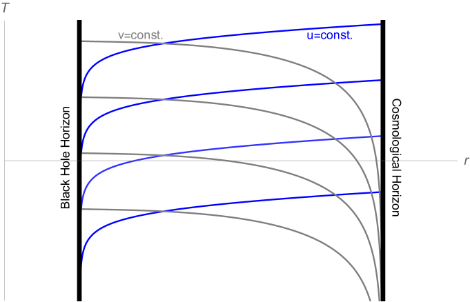
Figure 1: A plot showing how the null lines $u=t-r^{\star}=$const, $v=t+r^{\star}=$const appear in the $(T,r)$ coordinate system. Note how the $v$-lines meet the black hole horizon and the $u$-lines the cosmological horizon at finite $T$.

The constants $\gamma$ and $\beta$ are both positive, and the damping coefficient $3\gamma$ in the evolution equation (19) for the scalar field has a simple geometrical interpretation as the ratio of the sum of the black hole and cosmological horizon areas $A_{total}=4\pi(r_{c}^{2}+r_{b}^{2})$ to the thermodynamic volume $V_{dS}=4\pi(r_{c}^{3}-r_{b}^{3})/3$ from the SdS patch first law (9),

$$3\gamma=\frac{A_{total}}{V_{dS}}\,.$$ (29)

as was noted in Gregory:2017sor . The damping of the scalar field evolution is greatest for small $V_{dS}$, which corresponds to a large black hole with radius approaching that of the cosmological horizon.

II.3 Interlude on slow-roll approximation

Before proceeding with finding the solution, we outline more precisely the approximations within which we will be working. The resulting conditions on the potential are essentially the same as those in slow-roll inflation without a black hole Liddle:1993fq ; Liddle:1994dx , summarized in equations (32) and (34) below.

The picture is that we have a scalar potential with a shallow gradient so that the kinetic contribution of the scalar energy momentum tensor and the time-dependent corrections to $W$ are sub-dominant to the zeroth order contribution from the potential. In inflation, we summarise the slow-roll conditions in terms of the acceleration of the universe: “$\dot{H}/H<1$”. Here however we are in stationary coordinates for SdS spacetime, therefore we must identify our slow-roll in a slightly different way. However, the useful parameters turn out to be the same as the conditions familiar for typical inflationary models.

Similar to slow roll inflation, we will demand that the stress-energy is dominated by the contribution of the scalar potential, and that the $\ddot{\phi}$ term be subdominant to the $\dot{\phi}$ term in the scalar equation of motion. That is,

$$\frac{1-\eta^{2}}{f}{\dot{\phi}}^{2}\ll W\;\;,\qquad\frac{1-\eta^{2}}{f}{\ddot{\phi}}\ll\frac{1}{r^{2}}\left|\left(r^{2}\eta\right)^{\prime}\dot{\phi}\right|$$ (30)

Since ${\dot{\phi}}$ is assumed perturbatively small, the metric coefficients in the above relations can be taken to be their zeroth order values. Note that $(1-\eta^{2}_{0})/f_{0}$ is monotonically decreasing between the two horizons, and $(r^{2}\eta_{0})^{\prime}/r^{2}=-3\gamma$ is constant. Hence we can manipulate the first relation to give

$$\frac{1-\eta_{0}^{2}}{f_{0}}\frac{{\dot{\phi}}^{2}}{W}<-\frac{\eta^{\prime}(r_{b})}{\kappa_{b}}\frac{{\dot{\phi}}^{2}}{W}=\frac{2}{3\Lambda}\frac{(2r_{c}^{3}+3r_{c}^{2}r_{b}+r_{b}^{3})(r_{b}^{2}+r_{c}^{2}+r_{c}r_{b})}{(2r_{b}+r_{c})(r_{b}^{2}+r_{c}^{2})^{2}}\frac{W^{\prime 2}}{W}\simeq M_{p}^{2}\frac{W^{\prime 2}}{W^{2}}\ll 1$$ (31)

suggesting that we use the slow-roll parameter

$$\varepsilon=M_{p}^{2}\frac{W^{\prime 2}}{W^{2}}\ll 1$$ (32)

to quantify how “small” the kinetic term of the scalar is: $\dot{\phi}^{2}\lesssim\varepsilon W$.

For the second relation, we take the leading order approximation to the $\phi-$equation, (19), and differentiate to find $\ddot{\phi}$, giving

$$\left|\frac{1-\eta_{0}^{2}}{3\gamma f_{0}}\frac{\ddot{\phi}}{\dot{\phi}}\right|<\frac{2}{3\Lambda}\frac{(2r_{c}^{3}+3r_{c}^{2}r_{b}+r_{b}^{3})(r_{b}^{2}+r_{c}^{2}+r_{c}r_{b})}{(2r_{b}+r_{c})(r_{b}^{2}+r_{c}^{2})^{2}}W^{\prime\prime}\simeq M_{p}^{2}\frac{W^{\prime\prime}}{W}\ll 1$$ (33)

suggesting again that we use the parameter

$$\delta=M_{p}^{2}\frac{W^{\prime\prime}}{W}\ll 1$$ (34)

to quantify how small the variation of the kinetic term is: $\ddot{\phi}\lesssim\dot{\phi}\delta/r_{c}$. Note that this is again similar to the ‘eta’ parameter of the traditional slow-roll approach, here renamed as $\delta$.

We see therefore that the slow-roll relations are more or less the same as for the FRW cosmology without a black hole, however, the black hole introduces a radial dependence in the stationary patch coordinates that is easily bounded. The main difference between slow-roll with and without a black hole is the $\gamma-$parameter responsible for the friction of the scalar field. Since $\Lambda={\cal O}(r_{c}^{-2})$, $\gamma={\cal O}(\sqrt{\Lambda})/(1-r_{b}/r_{c})$ can be very much greater than the Hubble parameter that usually serves as the friction term in inflationary slow-roll, although it should be noted that the time with respect to which the scalar is rolling is the stationary patch time coordinate $T$.

III Solution for the Dynamical Metric

In the last section we analyzed the slow-roll evolution of a test scalar field $\phi$ with potential $W(\phi)$ in a background SdS spacetime. We found a suitable time coordinate $T$, such that there exist solutions $\phi=\phi(T)$ that are purely ingoing at the black hole horizon and outgoing at the cosmological horizon. Our next goal is to solve the back-reaction problem in perturbation theory to obtain the leading corrections to the SdS black hole metric as the scalar field rolls down its potential. We will present a preview of the results here and then provide their derivation in the next subsection. We start by making an ansatz for the form of the metric, taking the form of the SdS metric in the $(T,r)$ coordinates (27) but allowing the metric functions to depend on both the $T$ and $r$ coordinates

$$ds^{2}=-fdT^{2}+2\eta drdT+\frac{dr^{2}}{f}(1-\eta^{2})+r^{2}d\Omega^{2}$$ (35)

where $f=f(r,T)$ and $\eta=\eta(r,t)$. To be specific, we assume that the scalar field starts at time $T=T_{0}$ with a value $\phi_{0}$ corresponding to a maximum of the potential. The initial cosmological constant is given by $\Lambda_{0}=W(\phi_{0})/M_{p}^{2}$, and we assume that we start with an SdS black hole, so that the unperturbed metric has the form (27) with

$$f(r,T)=f_{0}(r;M_{0},\Lambda_{0})=1-\frac{2GM_{0}}{r}-\frac{\Lambda_{0}}{3}r^{2}$$ (36)

where $M_{0}$ is the initial black hole mass. Corresponding to the values of $M_{0}$, $\Lambda_{0}$ are initial values $r_{b0}$, $r_{c0}$ of the black hole and cosmological horizon radii, which in turn give the parameters $\beta$, $\gamma$ for the unperturbed SdS spacetime via (26).

Moving forward in time, the scalar field $\phi$ evolves via the scalar equation. In the background SdS spacetime, $\phi$ is constant, and therefore the time-dependent part of $\phi$ is perturbative and to leading order evolves according to the wave equation (19) in the background SdS spacetime. We note for future use that the time coordinate is related to the evolving scalar field by

$$T=-\frac{1}{3\gamma}\int\frac{d\phi}{(dW/d\phi)}$$ (37)

With this set-up, we can now state our results for the evolution of the spacetime geometry. The physical picture is that for slow-roll evolutions, the metric should transition through a progression of SdS metrics, with the parameters $M$ and $\Lambda$ varying slowly in time. We will show that the solutions come very close to realizing this expectation. Explicitly, we find that to leading order in perturbation theory, a metric of the form (35) satisfies the Einstein equations with stress-energy coming from the rolling scalar field, and metric functions given by

$$f=f_{QS}(r,T)+\delta f(r,T)\ ,\qquad\eta=\eta_{0}(r)+\delta\eta(T,r)$$ (38)

where

$$f_{QS}(r,T) =f_{0}\left(r;M(T),\Lambda(T)\right)=1-\frac{2GM(T)}{r}-\frac{\Lambda(T)}{3}r^{2}$$ (39)

$$\delta f(r,T) =-\frac{1}{2r}\frac{\dot{\phi}^{2}}{M_{p}^{2}}\int_{r_{b0}}^{r}\frac{1-\eta_{0}^{2}}{f_{0}}r^{\prime 2}dr^{\prime},\qquad\delta\eta(r,T)=\frac{r(1-\eta_{0}^{2})}{2f_{0}}\int_{T_{0}}^{T}\frac{\dot{\phi}^{2}}{M_{p}^{2}}dT$$

with

$$\dot{M}=\frac{dM}{dT}=4\pi\beta\dot{\phi}^{2},\qquad\dot{\Lambda}=-3\gamma\frac{\dot{\phi}^{2}}{M_{p}^{2}}$$ (40)

We will also demonstrate that the function $\delta f$ above is transient, and sub-dominant to the time dependent part of $f_{QS}(r,T)$. Thus the time dependent black hole and cosmological horizon radii $r_{h}(T)$ are well approximated by the zeros $r_{h}^{QS}(T)$ of the quasi-statically evolving portion $f_{QS}(r,T)$. By construction these zeros are related to the time dependent mass and cosmological constant $M(T)$ and $\Lambda(T)$ according to the SdS formulae in (7). Hence the time derivatives of $M(T)$ and $\Lambda(T)$ in (40) can be converted into time derivatives of the horizon radii $r_{h}(T)$, giving

$$\dot{r}_{h}=\frac{r_{h}}{2|\kappa_{h}|}\frac{\dot{\phi}^{2}}{M_{p}^{2}}\ ,\quad h=(b,c)$$ (41)

Expressions for the time dependent mass and cosmological constant can be obtained by using the integral

$$\int_{T_{0}}^{T}\dot{\phi}^{2}dT^{\prime}=-{1\over 3\gamma}\left[W(\phi(T))-W(\phi(T_{0}))\right]$$ (42)

Integrating $\dot{M}$, $\dot{\Lambda}$ and $\dot{r}_{h}$ using (42) we arrive at the results

$$\Lambda(T)\approx W(\phi(T))\ ,\qquad M(T)\approx M_{0}+{\beta\over 6\gamma}\left[W_{0}-W(\phi(T))\right]$$ (43)

and

$$r_{h}\approx r_{h0}+\frac{r_{h0}}{6\gamma|\kappa_{h}|}\left[W_{0}-W(\phi(T))\right]$$ (44)

and similarly for the function $\delta\eta(r,T)$ in (39). Note, we use the approximate equality above, as in the slow roll approximation it is possible for $M$ and $\Lambda$ to have additional slowly varying contributions (such as $\dot{\phi}^{2}$) whose derivatives are order $\ddot{\phi}$ or higher, and hence would not contribute to (40) at this order. We have denoted here $T_{0}$ as an initial time, which could be at $T_{0}\rightarrow-\infty$, when the scalar field is at the top of the potential with value $\phi_{0}$, the metric is SdS with mass parameter $M_{0}$, $\Lambda_{0}=W(\phi_{0})/M_{p}^{2}$, and the horizon radii are the corresponding $r_{h0}$ determined by (7). Note that the value of the scalar field potential, and hence the effective cosmological constant, is decreasing in time, so that the mass and both horizon radii are increasing functions of time.

III.1 Solving the Einstein equations

We now present the derivation of the quasi-de Sitter black hole solutions given above. With the assumption that $\phi=\phi(T)$, there are two independent components of the stress tensor,

$$T_{TT} =\left(W(\phi)+\frac{1+\eta^{2}}{2f}\dot{\phi}^{2}\right)|g_{TT}|\;,\qquad\text{and}$$ (45)

$$T_{\alpha\beta} =\left(-W(\phi)+\frac{1-\eta^{2}}{2f}\dot{\phi}^{2}\right)g_{\alpha\beta}\qquad\text{otherwise.}$$

and the Einstein tensor is:

$$G_{TT} =\left[\frac{1}{r^{2}}(1-f-rf^{\prime})-\frac{\eta\dot{f}}{rf}\right]|g_{TT}|$$ (46)

$$G_{rr} =\left[-\frac{1}{r^{2}}(1-f-rf^{\prime})+\frac{\eta\dot{f}}{rf}+\frac{2\dot{\eta}}{r(1-\eta^{2})}\right]g_{rr}$$

$$G_{rT} =\left[-\frac{1}{r^{2}}(1-f-rf^{\prime})-\frac{(1-\eta^{2})\dot{f}}{r\eta f}\right]g_{rT}$$

$$G_{\theta\theta} =\left[\frac{f^{\prime\prime}}{2}+\frac{f^{\prime}}{r}-\frac{\eta^{\prime}\dot{f}}{2f}+\frac{\dot{\eta}f^{\prime}}{2f}+\frac{\dot{\eta}}{r}+\dot{\eta}^{\prime}+\frac{1}{2}\left(\frac{(\eta^{2}-1)}{f}\right)^{\!\boldsymbol{\cdot}\boldsymbol{\cdot}}\right]g_{\theta\theta}=\frac{G_{\phi\phi}}{\sin^{2}\theta}$$

First consider the linear combination $\frac{G_{TT}}{|g_{TT}|}+\frac{G_{Tr}}{g_{Tr}}=M_{p}^{-2}\left(\frac{T_{TT}}{|g_{TT}|}+\frac{T_{Tr}}{g_{rT}}\right)$, which gives the relation

$$\dot{f}=-r\eta\,\frac{\dot{\phi}^{2}}{M_{p}^{2}}$$ (47)

and then $\frac{G_{TT}}{|g_{TT}|}+\frac{G_{rr}}{g_{rr}}=M_{p}^{-2}\left(\frac{T_{TT}}{|g_{TT}|}+\frac{T_{rr}}{g_{rr}}\right)$, which yields

$$\dot{\eta}=\frac{r(1-\eta^{2})}{2f}\,\frac{\dot{\phi}^{2}}{M_{p}^{2}}$$ (48)

thus both of our metric functions have a time-dependence determined by a radial profile times the kinetic energy of the scalar field. Since the quantity $\dot{\phi}^{2}$ is already perturbative, we need only consider the metric functions on the right hand sides of equations (47) and (48) to leading order, i.e. $f\to f_{0}$ and $\eta\to\eta_{0}$, the zeroth order SdS functions given in (5) and (28). So in perturbation theory, these equations give explicit expressions for the time evolution of $f$ and $\eta$.

Equations (47) and (48) can now be substituted back into the Einstein tensor in (46) to eliminate $\dot{f}$ and $\dot{\eta}$. One then finds that the $TT$, $Tr$, and $rr$ components of the normalized Einstein equation all reduce to

$$\frac{1}{r^{2}}(1-f-rf^{\prime})=\frac{W(\phi)}{M_{p}^{2}}+\frac{(1-\eta_{0}^{2})}{2f_{0}}\,\frac{\dot{\phi}^{2}}{M_{p}^{2}}$$ (49)

There remains the $\theta\theta$ equation, which using (47) and (48) becomes

$$-\frac{1}{2}f^{\prime\prime}-\frac{f^{\prime}}{r}=\frac{W}{M_{p}^{2}}+\frac{1}{2f_{0}}\left[(1-\eta_{0}^{2})-r\eta_{0}\eta_{0}^{\prime}-r(1-\eta_{0}^{2})f_{0}^{\prime}\right]\,\frac{\dot{\phi}^{2}}{M_{p}^{2}}$$ (50)

Taking the derivative with respect to $r$ of the Einstein equation (49) gives (50). So the equations of motion for the coupled Einstein scalar field system have been reduced to four equations, namely (47), (48) and (49), together with the slow-roll equation (19) for the scalar field.

Physical considerations now give insight as to the perturbative form of the metric functions $f(r,T)$ and $\eta(r,T)$. During slow roll evolution in an inflationary universe without a black hole the scalar field potential $W(\phi)$ provides a slowly varying effective cosmological constant. The stress-energy is dominated by the potential, with small corrections coming from the kinetic contribution of the scalar field. As the potential changes, the metric is approximately given by a progression of de Sitter metrics. With a black hole present, for sufficiently slow evolution, one expects that the metric will be close to an SdS metric with slowly evolving parameters $M(T)$ and $\Lambda(T)$. Looking at the expressions for the first three normalized components of the Einstein tensor (46), one sees that if $f=f_{0}$, then the terms in the first round parentheses are all proportional to $\Lambda_{0}$. Since these terms only depend on radial derivatives, if we use the ‘quasi-static’ metric function $f_{QS}(r,T)$ defined in (39) then these terms will be proportional to $\Lambda(T)$. Further, looking also at the normalized stress-energy components (45), one sees that the Einstein equations suggest a strategy of balancing $\Lambda(T)$ with $W[\phi(T)]$ and then equating the remaining terms. These are corrections to a pure cosmological equation of state from the kinetic energy of the scalar field.

Based on this reasoning, we adopt an ansatz of the form

$$f(r,T) =f_{QS}(r,T)+\delta f(r,T)$$ (51)

$$\eta(r,T) =\eta_{0}(r)+\delta\eta(r,T)$$

It may appear redundant to have the time dependence for $f$ explicit in both the function $f_{QS}(r,T)$, as well as $\delta f(r,T)$. However, it turns out this is a convenient way of packaging the time dependence implied by the Einstein equations in a physically relevant manner. One might also question the asymmetry in (51) between $f(r,T)$ and $\eta(r,T)$. However, this is simply what turns out to work. The next step is to substitute (51) into the Einstein equations, show that the ansatz allows a solution, and solve for the four functions $M(T)$, $\Lambda(T)$, $\delta f(r,T)$, and $\delta\eta(r,T)$.

Starting with $f(r,T)$, we substitute our ansatz into equations (49) and (47), to get

$$\Lambda(T)-{1\over r^{2}}\frac{\partial~{}}{\partial r}\left(r\delta f\right) = \frac{W\left[\phi(T)\right]}{M_{p}^{2}}+\frac{(1-\eta_{0}^{2})}{2f_{0}}\,\frac{\dot{\phi}^{2}}{M_{p}^{2}}$$ (52)

$$\frac{\dot{\Lambda}r^{2}}{3}+\frac{2G\dot{M}}{r}-\dot{\delta f} = \left(-\gamma r^{2}+\frac{\beta}{r}\right)\frac{\dot{\phi}^{2}}{M_{p}^{2}}$$ (53)

respectively. According to our physical picture, we try for a solution such that the cosmological constant tracks the value of the scalar potential, $\Lambda(T)=W[\phi(T)]/M_{p}^{2}$. Taking the time derivative of this, and using the slow-roll equation (19) for the scalar field, we get

$$\dot{\Lambda}(T)=-3\gamma\frac{\dot{\phi}^{2}}{M_{p}^{2}}\;,$$ (54)

consistent with the ${\cal O}(r^{2})$ terms in (53).

Next, we integrate (52) (after cancelling the $\Lambda$ and $W$ terms) to obtain

$$\delta f(r,T)=-\frac{1}{2r}\left(\int^{r}_{r_{b0}}dr^{\prime}(r^{\prime})^{2}\frac{1-\eta_{0}^{2}}{f_{0}}\right)\frac{\dot{\phi}^{2}}{M_{p}^{2}}$$ (55)

Here, we have chosen for convenience to fix the lower limit of the integral to be the initial black hole horizon radius $r_{b0}$, so that $\delta f(r_{0b},T)=0$; an alternate lower limit would correspond to a shift in $\delta f\propto\dot{\phi}^{2}/r$ that without loss of generality can be absorbed in $M(T)$ – recall that within the slow roll approximation, the rate of change of $\dot{\phi}^{2}$ is ignorable. Since second derivatives of $\phi$ are being neglected in the slow roll approximation, equation (55) implies that to this order

$$\frac{d~{}}{dT}\delta f\simeq 0$$ (56)

and hence we read off from (53)

$$\dot{M}(T)=4\pi\beta\,\dot{\phi}^{2}$$ (57)

This rate of change of $M$ corresponds to the accretion of scalar matter into the black hole. We have therefore demonstrated the quasi-static form of the solution for $f$, subject to the slowly varying $\delta f$.

It is interesting to compare this expression for $\dot{M}$ to that obtained for fluid accretion onto an asymptotically flat black hole by Babichev et al. Babichev:2005py ; Babichev:2012sg ,

$$\dot{M}(V)=-4\pi r^{2}T_{V}^{r}\;,$$ (58)

where $V$ is the Eddington-Finkelstein advanced time coordinate for the black hole, and we have used the more general expression from Babichev:2012sg to facilitate comparison. Taking the cosmological constant tending to zero, that is, $r_{b}\ll r_{c}$, we find that our expression for $T$ reduces to the Eddington-Finkelstein coordinate $V$, and $\beta\approx r_{b}^{2}$. Finally, using the expression for the energy momentum tensor, $\dot{\phi}^{2}=-T_{V}^{r}$ giving precisely the expression (58) of Babichev et al.

Finally, we integrate (48) to obtain

$$\delta\eta(r,T)=\frac{r(1-\eta_{0}^{2})}{2f_{0}}\int_{T_{0}}^{T}\frac{\dot{\phi}^{2}}{M_{p}^{2}}dT^{\prime}+\eta_{1}(r,T)$$ (59)

where $\eta_{1}$ is a slowly varying function ($\dot{\eta}_{1}\approx 0$) that will turn out to be proportional to $\dot{\phi}^{2}$, and we require that $\delta\eta$ is zero at the start of the slow roll process $T_{0}$.

This completes the derivation of the slow-roll solution. The evolution of all the functions, $M(T)$, $\Lambda(T)$, $\delta f(r,T)$, and $\delta\eta(r,T)$ in the quasi-SdS metric (51) are determined in terms of the unperturbed SdS metric and $\dot{\phi}(T)$, which is in turn determined through the slow roll equation (19) by the slope $dW/d\phi$ of the scalar potential. While the quasi-SdS solution is not quite as simple as the static SdS spacetime, we will see that the quasi-SdS form allows us to study the thermodynamics of both the black hole and cosmological horizons in an intuitive way.

IV Horizons

In this section we locate the horizons $r_{h}(T)$ of the dynamical metric. In the background static SdS metric, $M_{0}$ and $\Lambda_{0}$ are related to the horizon radii $r_{b0}$ and $r_{c0}$ by the formulae (7). Since our solutions almost track a sequence of SdS metrics we expect that the black hole and cosmological horizons are given by almost the same SdS formulae, with $M(T)$ and $\Lambda(T)$ replacing the constant parameters. However, “almost” is the operative word, since both $f$ and $\eta$ receive modifications. Nonetheless, our findings are that:

$\bullet$ After an initial time period, the $\delta f$ corrections become negligible;

$\bullet$ $\eta(T,r)$ still satisfies the needed boundary conditions, and as a result,

$\bullet$ the simple quasi-static formulae for the horizon radii apply after that initial period.

The derivation proceeds in two steps. We first find the time dependent zeros of $f(T,r)$ and identify the “start up” time interval. Second, we look at the form of the metric near the zeros of $f$ and show that these are horizons. We close this section by comparing the results to those in our previous paper Gregory:2017sor which used a different coordinate system for the evolving system.

IV.1 Finding zeros of $f(r,T)$

Here we show that after an initial time period estimated below, the horizons $r_{h}(T)$ are given by the zeros of $f_{QS}$, that is, the $r_{h}(T)$ with $h=(b,c)$, have the same algebraic relation to $M(T)$ and $\Lambda(T)$ as do the quantities in static SdS. In the unperturbed SdS spacetime, the black hole and cosmological Killing horizons are located at the zeros of $f_{0}(r)$, so we start by finding the zeros of $f(r,T)$, which we designate by $r_{z,h}(T)$. That is,

$$f\left(r_{z,h}(T),T\right)=0$$ (60)

where $f(r,T)$ is given in equation (38) by

$$f(r,T)=f_{QS}(r,T)-\frac{1}{2r}\frac{\dot{\phi}^{2}}{M_{p}^{2}}I(r)$$ (61)

with

$$I(r)=\int_{r_{b0}}^{r}\frac{(1-\eta_{0}^{2})}{f_{0}}r^{\prime 2}dr^{\prime}$$ (62)

Denote the zeroes of the quasi-static metric function $f_{QS}(r,T)$, defined in (39), as $r_{h}^{QS}(T)$, so that

$$f_{QS}\left(r_{h}^{QS}(T),T\right)=0$$ (63)

It follows that the quasi-static radii $r_{h}^{QS}(T)$ are given in terms of the time dependent mass and cosmological constant parameters $M(T)$ and $\Lambda(T)$ by the SdS relations (7).

Let us now compare the $r_{z,h}(T)$ to the $r_{h}^{QS}(T)$. Since by construction $I(r_{b0})=0$, these two types of zeroes coincide at the black hole horizon,

$$r_{z,b}(T)=r_{b}^{QS}(T)$$ (64)

On the other hand, when $r=r_{c0}$ in $I$, equation (60) becomes

$$-\frac{\Lambda(T)}{3}r_{z,c}^{3}+r_{z,c}-2GM(T)-\frac{1}{2}\frac{\dot{\phi}^{2}}{M_{p}^{2}}I(r_{c0})=0$$ (65)

which is not the same as the condition (63). Hence, the radii $r_{c}^{QS}(T)$ and $r_{z,c}(T)$ differ, with the difference arising from $I(r_{c0})$, which enters the polynomial equation (65) as a contribution to the time dependence of the mass term $M(T)$. Let us compare the magnitudes of the last two terms in (65). One might be concerned that $I(r_{c0})$ would diverge due to the factor of $1/f_{0}$ in the integrand in (62). However, the zeros of $1-\eta_{0}^{2}$ cancel the zeros of $f_{0}$ at $r_{b0}$ and $r_{c0}$. Explicitly,

$$1-\eta_{0}=\frac{(r-r_{b0})}{(r_{c0}^{3}-r_{b0}^{3})r^{2}}P(r,r_{b0},r_{c0})\ ,\quad 1+\eta_{0}=\frac{(r_{c0}-r)}{(r_{c0}^{3}-r_{b0}^{3})r^{2}}P(r,r_{c0},r_{b0})$$ (66)

where $P(r,d,e)=r^{2}(d^{2}+e^{2})+re^{2}(d+e)+de^{2}(d+e)$. Therefore the integral may be rewritten as

$$I(r)=\frac{3}{\Lambda(r_{c0}^{3}-r_{b0}^{3})^{2}}\int_{r_{b0}}^{r}dr^{\prime}\frac{P(r^{\prime},r_{b0},r_{c0})P(r^{\prime},r_{c0},r_{b0})}{r^{\prime}(r^{\prime}-r_{N})}$$ (67)

which is manifestly finite at $r=r_{c0}$. So the final term in (65) is then proportional to the instantaneous value of $\dot{\phi}^{2}$ times this finite, time-independent, quantity, while from (40) we know that the change in $M(T)$ from its initial value $M_{0}$ depends on the accumulated change of $\dot{\phi}^{2}$ integrated over time (plus a possible slowly varying term). Therefore, after a start up time the contribution to $r_{z,c}$ coming from $\dot{\phi}^{2}I(r_{c0})$ will be small compared to the contribution from the evolution of $[M(T)-M_{0}]$. Explicit comparison of these terms shows that the shift due to the $I(r_{c0})$ term is negligible after a time interval $(T-T_{0})\simeq r_{b0}\ln(r_{c0}/r_{b0})$ for small black holes with $r_{b0}\ll r_{c0}$, and after $(T-T_{0})\simeq r_{b}$ for large black hole with $r_{b0}$ of order $r_{c0}$. Note that if the initial time $T_{0}$ is taken to be $-\infty$ then the extra term is irrelevant. After this initial time period the zeros of $f(r,T)$ coincide with the zeros of $f_{QS}(r,T)$

$$r_{z,b}(T)=r_{b}^{QS}(T)\ ,\quad r_{z,c}(T)=r_{c}^{QS}(T)$$ (68)

and hence evolve in a quasi-static way determined by the evolution of the quasi-SdS parameters $M(T)$ and $\Lambda(T)$. It may seem odd that the additional function $\delta f$ is needed to solve the Einstein equation at early times, rather than at late times. This likely illustrates the teleological nature of the horizon, as it starts to grow in anticipation of the influx of stress-energy from the evolving scalar field. This effect was also noticed in a simpler inflationary example with no black hole in Gregory:2017sor .

IV.2 Near horizon behavior

In this section we find the form of the metric near the zeros of $f$ and show that it takes the form of a black hole or cosmological horizon. This then implies that the functions $r_{z,h}(T)$ do locate the horizons, and combining with the results of the previous section, we will have demonstrated that the horizon radii evolve quasi-statically,

$$r_{h}(T)=r_{z,h}(T)\simeq r_{h}^{QS}(T)$$ (69)

after an initial period as discussed above.

Let us recall what the horizons look like in the static SdS metric, starting with the static time coordinate $t$, and $r$. Defining the radial tortoise coordinate by $dr^{\star}=dr/f_{0}$ and the ingoing Eddington-Finklestein coordinate at the black hole horizon by $v=t+r^{\star}$, the SdS metric near the black hole horizon is approximately given by

$$ds^{2}\simeq-2\kappa_{b}(r-r_{b})dv^{2}+2drdv+r^{2}d\Omega^{2}$$ (70)

Although the metric component $g_{vv}\simeq-2\kappa_{b}(r-r_{b})dv^{2}$ vanishes at the horizon, the metric is non-degenerate there. The vector $\partial/\partial v$ is null and ingoing at the horizon. To study the cosmological horizon, one uses outgoing coordinates with $u=t-r^{\star}$. Then near the cosmological horizon the metric becomes

$$ds^{2}\simeq 2|\kappa_{c}|(r-r_{c})dv^{2}-2drdu+r^{2}d\Omega^{2}$$ (71)

The vector field $\partial/\partial u$ is outgoing and null at the horizon and the cross term in the metric changes sign.

One can also look at the metric near the horizons of SdS using the the stationary coordinate $T$ given in (14). As noted earlier, $T$ interpolates between the ingoing null Eddington-Finklestein coordinate $v$ on the black hole horizon, and the outgoing null coordinate $u$ on the cosmological horizon. So there is no need to transform the coordinates, we just look at the metric functions near the horizons. As $r\rightarrow r_{b}$ the SdS metric becomes

$$ds^{2}\simeq-2\kappa_{b}(r-r_{b})dT^{2}+2dTdr+\frac{C_{b}}{\kappa_{b}}dr^{2}+r^{2}d\Omega^{2}\$$ (72)

where $C_{b}=-\eta^{\prime}_{0}(r_{b})=(2r_{c}^{3}+3r_{c}^{2}r_{b}+r_{b}^{3})[r_{b}(r_{c}^{3}-r_{b}^{3})]^{-1}\ >0$. The essential difference between (70) and (72) is that $g_{rr}=0$ in the $(v,r)$ coordinates, while $g_{rr}$ is non-zero but finite in the $(T,r)$ coordinates. This is due to the fact that $T$ is not identical to $v$ near $r_{b}$. Similarly, near the cosmological horizon of SdS the metric in stationary cooordinates has the form

$$ds^{2}\simeq 2|\kappa_{c}|(r-r_{c})dT^{2}-2dTdr+\frac{C_{c}}{|\kappa_{c}|}dr^{2}+r^{2}d\Omega^{2}\$$ (73)

and one sees explicitly that $T$ has become an outgoing null coordinate. Here $C_{c}=-\eta^{\prime}_{0}(r_{c})>0$.

The analysis of the time-dependent metric in (38) near the zeros of $f$ proceeds in a similar way. Take the time $T$ to be sufficiently large that the zeros of $f$ are well approximated by the zeros of $f_{QS}$. Further, to avoid repetition of bulky notation, we will simply abbreviate $r_{h}^{QS}(T)=r_{h}(T)$, and the end result justifies this replacement. As $r$ approaches $r_{b}(T)$, the metric function $f$ behaves like

$$f\simeq-2\kappa_{b}(T)\left(r-r_{b}(T)\right)$$ (74)

where $\kappa_{b}(T)$ is defined as the derivative

$$\kappa_{b}(T)={1\over 2}f^{\prime}|_{r=r_{b}(T)}$$ (75)

At present we will not ascribe any significance to $\kappa_{b}(T)$ as a possible time-dependent surface gravity or temperature.

The behavior of the metric function

$$g_{rr}=\frac{(1-\eta^{2})}{f}$$ (76)

in the time dependent solution (38) appears to be more subtle, since although the zeros of $f$ in the denominator are cancelled by zeros in the numerator for exact SdS, it is not immediately obvious whether this is still true for the perturbed functions $f$ and $\eta$. However, (47) and (48) together imply that $g_{rr}$ is in fact independent of $T$, provided only that $\phi=\phi(T)$, hence $g_{rr}$ remains regular even if the locations of the zeros of $f$ shift. Let us now confirm this, by deriving explicitly the locations of these zeros. Denote $r_{h0}$ as an horizon radius in the unperturbed SdS spacetime (a zero of $f_{0}$) and expand the time-dependent horizon radius around this as

$$r_{h}(T)=r_{h0}+x_{h}(T)$$ (77)

where the shift in the position of the zero is assumed small, $|x_{h}|/r_{h0}\ll 1$. $r_{h}(T)$ is defined as a zero of $f(r,T)$, therefore $x_{h}$ can be deduced by Taylor expanding the relation $f(T,r_{h}(T))=0$ around $r_{h0}$ and using the expression we have derived for $f(r,T)$, yielding

$$x_{h}(T)=\frac{r_{h}}{2\kappa_{h}}\eta_{0}(r_{h})\int_{T_{0}}^{T}\frac{\dot{\phi}^{2}}{M_{p}^{2}}dT^{\prime}-\frac{I(r_{h})}{2r_{h}}\frac{\dot{\phi}^{2}}{M_{p}^{2}}$$ (78)

thus verifying (44). Expanding $\eta$ near each horizon similarly shows

$$\eta(r_{h}(T)) =\eta_{0}(r_{h})+x_{h}\eta_{0}^{\prime}(r_{h})+\frac{r_{h}(1-\eta_{0}^{2})}{2f_{0}}\int_{T_{0}}^{T}\frac{\dot{\phi}^{2}}{M_{p}^{2}}+\eta_{1}(r_{h},T)$$ (79)

$$=\eta_{0}(r_{h})+\eta_{1}(r_{h},T)-\frac{I(r_{h})}{2r_{h}}\frac{\dot{\phi}^{2}}{M_{p}^{2}}$$

i.e. fixing $\eta_{1}=I(r)\dot{\phi}^{2}/2rM_{p}^{2}$, we have that $\eta(r_{h}(T))=\eta_{0}(r_{h0})=\pm 1$, explicitly confirming that $g_{rr}$ remains regular at the new horizon radii.

Therefore although the metric function $g_{TT}$ vanishes at $r_{h}(T)$, the metric is non-degenerate there, as was the case in the unperturbed SdS spacetime. The cross term $+2dTdr$ in the metric at the black hole horizon illustrates the ingoing nature of the $T$ coordinate near that horizon, where it becomes a null coordinate that is well-behaved, a property that was built into the choice of $T$ to ensure ingoing boundary conditions for $\phi(T)$. A similar analysis applies to the cosmological horizon as $r$ approaches $r_{c}(T)$. The cross term in the metric in this case will have the opposite sign illustrating the outgoing nature of the coordinate $T$ near the cosmological horizon.

The preceeding subsections are summarized by the formula for $r_{h}(T)$ given in (44), valid after an initial start-up time.

IV.3 Calculation in null coordinates

In this subsection we show that these results for the growth of the horizon radii agree with the calculations in our previous paper Gregory:2017sor . This is a useful exercise since the first paper worked in null coordinates, in which it was simple to locate the horizons but difficult to find the metric throughout the region. In contrast, the coordinates used in the current paper allow us to find the metric straightforwardly, but the horizon structure requires more work. Comparison requires further processing of the results of Gregory:2017sor using the slow-roll approximation requirements derived earlier.

In Gregory:2017sor , we showed that the linearized Einstein equations on the horizon reduced to simple second order ODE’s in terms of the advanced time coordinate $V_{b}$ on the black hole horizon, and $U_{c}$ on the cosmological horizon:

$$\frac{d^{2}~{}~{}}{dV_{b}^{2}}\delta{\cal A}_{b}=-\frac{{\cal A}_{b}}{\kappa_{b}^{2}M_{p}^{2}}\frac{\dot{\phi}^{2}}{V_{b}^{2}}\;,\qquad\frac{d^{2}~{}~{}}{dU_{c}^{2}}\left(U_{c}\delta{\cal A}_{c}\right)=-\frac{{\cal A}_{c}}{\kappa_{c}^{2}M_{p}^{2}}\frac{\dot{\phi}^{2}}{U_{c}}$$ (81)

where ${\cal A}_{h}$ is the area of the respective horizon. In the background SdS metric, these coordinates are related to $T$ by

$$\kappa_{b}V_{b}=\exp[\kappa_{b}(T-T_{0})]\;,\qquad\kappa_{c}U_{c}=\exp[\kappa_{c}(T-T^{\prime}_{0})]$$ (82)

Integrating (81) gave the general expressions for the horizon areas, from which we can deduce the values of horizon radii as

$$\delta r_{b} =-\frac{r_{b}}{6\gamma\kappa_{b}M_{p}^{2}}V_{b}\int_{V_{b}}^{\infty}\delta W[\phi(V_{b}^{\prime})]\frac{dV_{b}^{\prime}}{V_{b}^{\prime 2}}$$ (83)

$$\delta r_{c} =-\frac{r_{c}}{6\gamma\kappa_{c}M_{p}^{2}U_{c}}\int^{0}_{U_{c}}\delta W[\phi(U_{c}^{\prime})]dU_{c}^{\prime}$$

At first sight, these look somewhat different from the values of $\delta r_{h}$ obtained from (44), however, armed with the slow roll analysis for integrating the Einstein equations, let us re-examine these expressions. Integrating by parts in $\delta r_{b}$, and using $\kappa_{b}V_{b}=\exp[\kappa_{b}(T-T_{0})]$ we find

$$\delta r_{b}=-\frac{r_{b}}{6\gamma\kappa_{b}M_{p}^{2}}\left[\delta W[\phi(V_{b})]-3\gamma e^{\kappa_{b}T}\int_{T}^{\infty}\dot{\phi}^{2}e^{-\kappa_{b}T^{\prime}}dT^{\prime}\right]$$ (84)

Similarly, the $r_{c}$ equation can be integrated by parts to give

$$\delta r_{c}=-\frac{r_{c}}{6\gamma\kappa_{c}M_{p}^{2}}\left[-\delta W[\phi(U_{c})]+3\gamma e^{-\kappa_{c}T}\int_{T}^{\infty}\dot{\phi}^{2}e^{\kappa_{c}T^{\prime}}dT^{\prime}\right]$$ (85)

To approximate these integrals, we use (34) to compare how rapidly $\dot{\phi}^{2}$ is varying compared to the exponential, in other words, the magnitude of

$$\left|\frac{1}{\dot{\phi}^{2}\kappa_{h}}\frac{d~{}}{dT}\dot{\phi}^{2}\right|=\left|\frac{W^{\prime\prime}}{\gamma\kappa_{h}}\right|=\frac{r_{c}^{2}+r_{c}r_{b}+r_{b}^{2}}{r_{c}^{2}+r_{b}^{2}}\frac{4r_{h}\delta}{2r_{h}+r_{\bar{h}}}<3\delta\ll 1$$ (86)

(where the ‘$\bar{h}$’ subscript stands for ‘the other’ horizon). Thus $\dot{\phi}^{2}$ varies much more slowly than the exponential, and we can approximate each of these integrals by $\dot{\phi}^{2}e^{-|\kappa_{h}|T}/|\kappa_{h}|$ yielding

$$\delta r_{h}\simeq-\frac{r_{h}}{6\gamma|\kappa_{h}|M_{p}^{2}}\left[\delta W-\frac{3\gamma}{|\kappa_{h}|}\dot{\phi}^{2}\right]$$ (87)

Let us now compare these two terms. At the start of slow-roll, i.e. at the local maximum of $W$,

$$W\simeq W_{0}+\frac{1}{2}W^{\prime\prime}\delta\phi^{2}\;\;\Rightarrow\quad\delta\phi\propto e^{-W^{\prime\prime}T/3\gamma}\;\;{\rm as}\;\;T\to-\infty$$ (88)

hence

$$\left|\frac{3\gamma\dot{\phi}^{2}}{\kappa_{h}\delta W}\right|=\left|\frac{2W^{\prime\prime}}{3\kappa_{h}\gamma}\right|<2\delta\ll 1$$ (89)

thus $\delta W$ is initially the dominant term in (87). Moreover, throughout slow-roll, examining the rate of change of each term,

$$\dot{\delta W}=-3\gamma\dot{\phi}^{2}\;\;,\quad\left(\frac{3\gamma\dot{\phi}^{2}}{\kappa_{h}}\right)^{\!\boldsymbol{\cdot}}=-3\gamma\dot{\phi}^{2}\frac{2W^{\prime\prime}}{\kappa_{h}\gamma}\;\;\;\Rightarrow\quad\left|\left(\frac{3\gamma\dot{\phi}^{2}}{\kappa_{h}}\right)^{\!\boldsymbol{\cdot}}\right|\ll\left|\dot{\delta W}\right|$$ (90)

shows that if $\delta W$ is dominant initially, it will remain so throughout the transition between vacua, meaning that the evolution of the horizon area is dominated by the shift in the cosmological constant which is the first term in (87), in agreement with (44).

V Horizon areas, black hole mass, and first laws

In this section we compute the rates of change for the areas of the black hole and cosmological horizons, the black hole mass, and the thermodynamic volume between the horizons. We then show that the de Sitter patch first law (9) and the mass first law (12) are satisfied throughout the evolution. In our previous paper Gregory:2017sor we showed that (9) held between the initial and final SdS states, relating the total changes in these quantities over the evolution. In this earlier work we lacked the detailed form of the time dependent metric and were unable to verify the mass first law equation, though we inferred the value of the late time mass based on assuming that the mass first law was true. Here, equipped with the solution for the metric (38), we are able to do more.

V.1 Horizon area growth and first law

$A\ priori$ one expects that the black hole horizon area should be increasing in time due to accretion of scalar field stress-energy. However, for the cosmological horizon there are competing influences on its area that tend in opposite directions. For fixed $\Lambda$ the cosmological horizon gets pulled in as the black hole mass grows, while for fixed black hole mass the cosmological horizon grows as $\Lambda$ shrinks. The solutions showed that both horizon radii are increasing, so the latter effect dominates the behavior of the cosmological horizon.

Throughout this section we will work in the late time limit defined above in §IV.1, so the black hole and cosmological horizons are located at the zeros of the quasi-static metric function $f_{QS}(r,T)$. This implies that $r_{b}(T)$ and $r_{c}(T)$ are given in terms of the time dependent mass $M(T)$ and vacuum energy $\Lambda(T)$ by the same relations (7) that apply in the unperturbed SdS spacetime. The expressions for $\dot{M}$ and $\dot{\Lambda}$ in the time dependent solution (38) then yield the expressions given in (41) for $\dot{r_{b}}$ and $\dot{r_{c}}$. It follows that the rate of change of the black hole and cosmological horizon areas is

$$\dot{A}_{h}=\frac{A_{h}}{|\kappa_{h}|}\frac{\dot{\phi}^{2}}{M_{p}^{2}}\ ,\quad\quad h=(b,c)$$ (91)

Now it can be checked that the SdS-patch first law (9) holds in a dynamical sense. Summing the expressions for the rate of growth of the horizon areas (91) gives

$$|\kappa_{b}|\dot{A_{b}}+|\kappa_{c}|\dot{A_{c}}=A_{tot}\frac{\dot{\phi}^{2}}{M_{p}^{2}}$$ (92)

Using the formulae for $\dot{\Lambda}$ in (40) and the thermodynamic volume of the de Sitter patch $V_{dS}$, equation (29), gives

$$V\dot{\Lambda}=-A_{tot}\frac{\dot{\phi}^{2}}{M_{p}^{2}}$$ (93)

and so

$$|\kappa_{b}|\dot{A_{b}}+|\kappa_{c}|\dot{A_{c}}=-V\dot{\Lambda}$$ (94)

Interpreting the variations in (9) as time derivatives, and translating $|\kappa_{h}|M_{p}^{2}\delta A_{h}=T_{h}\delta S_{h}$, we see that the SdS-patch first law (9) holds between successive times. Hence the decrease of the effective cosmological constant due to the scalar field rolling down its potential goes into increasing the black hole and cosmological horizon entropies.

It is also straightforward to check that the mass first law (12) is satisfied throughout the evolution for the time dependent solutions. Plugging in for $\dot{M}$ and $\dot{\Lambda}$ using (38), and $\dot{A}_{b}$ using (91), one finds that the mass first law reduces to the first relation in (25), that is, the evolution satisfies

$$\frac{\dot{M}}{M_{p}^{2}}-|\kappa_{b}|\dot{A}_{b}+V_{b}\dot{\Lambda}=0$$ (95)

The accumulated growth in time for each horizon is obtained by integrating the expressions (91) for $\dot{A_{h}}$, which at late times gives

$$\delta A_{h}(T)=-\frac{A_{h}V_{dS}}{3|\kappa_{h}|A_{tot}}\delta\Lambda$$ (96)

where $\delta A_{h}(T)\equiv A_{h}(T)-A_{h0}$ and $\delta\Lambda=\Lambda_{0}-\Lambda[\phi(T)]$. The prefactors all refer to values in the initial SdS spacetime, and keeping in mind that $\delta\Lambda(T)$ is negative, $\delta A_{h}$ is positive. Hence the change in area of each horizon between $T_{0}$ and $T$ is proportional to the initial horizon area times the change in the effective cosmological constant. It is also interesting to note that during the evolution that the fractional increase in area, times the magnitude of the surface gravity, is the same for both horizons

$$|\kappa_{c}|\frac{\delta A_{c}}{A_{c}}=|\kappa_{b}|\frac{\delta A_{b}}{A_{b}}$$ (97)

The geometrical quantities appearing in equation (96) are not all independent. The initial SdS spacetime is specified by two parameters, which we have been taking to be the initial black hole horizon radius and the initial value of the potential, and so one wants formulae that only depend on $r_{b}$ and $\Lambda$. Substituting in the surface gravity and thermodynamic volume gives, for the black hole horizon,

$$\delta A_{b}=A_{b}\frac{|\delta\Lambda|}{\Lambda}\ \frac{2r_{b}(r_{c}^{2}+r_{b}^{2}+r_{c}r_{b})}{(2r_{b}+r_{c})(r_{b}^{2}+r_{c}^{2})}$$ (98)

The corresponding expression for $\delta A_{c}$ is obtained by interchanging $r_{b}$ and $r_{c}$. In (98) $r_{c}$ is still an implicit function of $r_{b}$ and $\Lambda$. We will display the results in the limits of small and large black holes. For the black hole horizon area one finds

$$\delta A_{b}\simeq\begin{cases}A_{b}\frac{2|\delta\Lambda|}{\sqrt{3}\Lambda}\ \sqrt{\Lambda r_{b}^{2}}\ ,\qquad\qquad&\sqrt{\Lambda r_{b}^{2}}\ll 1\\ A_{b}\frac{|\delta\Lambda|}{\Lambda}\ ,&\sqrt{\Lambda r_{b}^{2}}\sim 1\end{cases}$$ (99)

One sees that the fractional growth is parametrically suppressed for small black holes, and of order $|\delta\Lambda|/\Lambda$ for large ones. Likewise, one can examine how much the growth of the cosmological horizon is suppressed by the presence of the black hole. One finds

$$\delta A_{c}\simeq\begin{cases}12\pi\frac{|\delta\Lambda|}{\Lambda^{2}}\ ,\qquad\qquad&\sqrt{\Lambda r_{b}^{2}}\ll 1\\ 4\pi\frac{|\delta\Lambda|}{\Lambda^{2}}\ ,&\sqrt{\Lambda r_{b}^{2}}\sim 1\end{cases}$$ (100)

The small black hole result is the same as if there were no black hole. On the other hand, the growth of the area of the cosmological horizon can be diminished by as much as a factor of two-thirds for large black holes. This suggests that the effect of a large black hole on the spectrum of CMBR perturbations created during slow roll inflation is worthy of further study.

While both horizon areas increase, the black hole gets smaller compared to the cosmological horizon in certain ways. The volume $V_{dS}$ between the horizons increases according to

$$\dot{V}_{dS}=2\pi\left(\frac{r_{c}^{3}}{|\kappa_{c}|}-\frac{r_{b}^{3}}{|\kappa_{b}|}\right)\frac{\dot{\phi}^{2}}{M_{p}^{2}}$$ (101)

Since $|\kappa_{c}|<\kappa_{b}$ McInerney:2015xwa the right hand side is positive. Another measure is how the difference between the black hole and cosmological horizon areas changes in time:

$$A_{c}(T)-A_{b}(T)-(A_{c0}-A_{b0})=\delta A_{c}-\delta A_{b}=24\pi\frac{|\delta\Lambda(T)|}{\Lambda^{2}}\frac{(r_{c}-r_{b})(r_{c}+r_{b})^{3}}{(r_{c}^{2}+r_{b}^{2})(2r_{c}+r_{b})(2r_{b}+r_{c})}$$ (102)

Since $|\delta\Lambda(T)|$ increases with time, the black hole is getting smaller in comparison to the cosmological horizon. To unravel the parameter dependence of (102), we again look at different limiting cases

$$\delta A_{c}-\delta A_{b}\simeq\begin{cases}12\pi\frac{|\delta\Lambda|}{\Lambda^{2}}\ \sqrt{\Lambda r_{b}^{2}}\ ,\qquad\quad\quad&\sqrt{\Lambda r_{b}^{2}}\ll 1\\ 6\pi\frac{|\delta\Lambda|}{\Lambda^{2}}\ ,&r_{b}={1\over 2}r_{c}\\ \frac{32\pi}{3}\frac{|\delta\Lambda|}{\Lambda^{2}}(1-\sqrt{\Lambda r_{b}^{2}})\ \ ,&\sqrt{\Lambda r_{b}^{2}}\sim 1\end{cases}$$ (103)

We see in this case that the effect is parametrically suppressed both for very small and very large black holes and most prominent in the intermediate regime.

V.2 Dynamical temperature

We have not yet discussed horizon temperature for the time dependent quasi-SdS black holes (38). These represent non-equilibrium systems, for which it is not clear that a well-defined notion of dynamical temperature should exist. Nevertheless, given that our system is only slowly varying, we might expect that an adiabatic notion of temperature makes sense GalvezGhersi:2011tx ; Barcelo:2010pj and indeed candidate definitions have been suggested in the literature. We will focus, in particular, on the proposal Hayward:2008jq which defines a dynamical surface gravity $\kappa_{dyn}$ for outer trapping horizons in nonstationary, spherically symmetric spacetimes. In this construction, the Kodama vector Kodama:1979vn substitutes for the time translation Killing vector of a stationary spacetime in providing a preferred flow of time. Further, the authors use a variant of the tunneling method of Parikh:1999mf , adapted to the non-stationary setting, to argue that particle production has a thermal form with temperature $T_{dyn}=\kappa_{dyn}/2\pi$.

The dynamical surface gravity is defined in Hayward:2008jq as

$$\kappa_{dyn}=\frac{1}{2}\star d\star dr$$ (104)

where the Hodge $\star$ refers to the two dimensional $T,r$ subspace orthogonal to the $2$-sphere, and the quantity is to be evaluated at the horizon. The Hodge duals of the relevant forms are given by

$$\star dr=fdT-hdr\ ,\qquad\star dr\wedge dT=1$$ (105)

Using these expressions, and evaluating (104) on the black hole horizon, one finds that

$$\kappa_{dyn}(T)=(f^{\prime}+\dot{\eta})=\kappa_{b}(T)+{\cal O}(\varepsilon\delta)$$ (106)

where $\kappa_{b}(T)$ was defined in equation (75) as the derivative of the perturbed metric function $f(r,T)$ evaluated at radius $r_{b}(T)$. Note that although the contribution $\delta f(r,t)$ to the metric function vanishes at $r_{b0}$, its derivative is non-zero and therefore $\kappa_{b}(T)$ gets contributions both from $f_{QS}$ and from $\delta f$, with the result that

$$\kappa_{b}(T)=\kappa_{QS}(T)-\frac{C_{b}}{2\kappa_{b}}\dot{\phi}^{2}$$ (107)

Here the quasi-static surface gravity $\kappa_{QS}(T)$ is given by the SdS relation (8) using $r_{b}(T)$ and $r_{c}(T)$, and expanding to linear order in the perturbative quantities. These time-dependent corrections to the radii $r_{h}(T)$ are proportional to the integral over time of $\dot{\phi}^{2}$, but the second term in (107) depends on the instantaneous value of $\dot{\phi}^{2}$. So after an initial time period the latter term is small compared to the first, and the dynamical surface gravity is well approximated by

$$\kappa_{b}(T)\simeq\kappa_{QS}(T)$$ (108)

We see that the proposal of Hayward:2008jq yields a simple, intuitive result. This is in agreement with our results in Gregory:2017sor where the calculation was done using null coordinates.

VI Conclusion

In this paper we have found a tractable form for the metric of a black hole in a slow-roll inflationary cosmology, to first order in perturbation theory, which one can readily understand in terms of expectations for the slowly evolving system. The solution directly gives the time dependence of $\Lambda$ and $M$ and it is straightforward to then find the time dependent horizon areas, the thermodynamic volume, and the dynamical surface gravity. A topic for future study is to compute the flux of the energy-momentum of the scalar field across surfaces of constant $r$. The flux is ingoing at the black hole horizon, and outgoing at the cosmological horizon, and it would be good to understand our results for the growth of the horizons and the mass in terms of the fluxes in greater detail, as was done in Chadburn:2013mta . Further, there must be a transition surface between the horizons where the flux vanishes, so mapping out the flux throughout the domain would be of interest. A related issue is to look at the energy density and pressure variation across spatial slices that interpolate to a standard inflationary cosmology in the far field. The range of validity of the approximate solution we have derived is another issue for further study. Conservatively, one assumes that $|\delta\Lambda/\Lambda|$ must be small. However, since the slow-roll conditions require that the derivatives of the potential must be small, one might ask if larger accumulated change in $W$ is allowed, as long as the evolution is slow enough. In any case, our approximation is equally valid as the slow roll approximation in the inflationary evolution of the early universe.

It is of interest to calculate the perturbations from inflation with the black hole present, as such signatures in the CMBR may be a method for detecting, or inferring, primordial black holes Afshordi:2017use . Although the black hole itself is small-scale, the wavelength of its signature on modes that re-enter the horizon at late times is stretched with the modes themselves. A related problem is to compute the Hawking radiation in this metric by extending the methods of Kastor:1993mj to the quasi-static case. Such a calculation is needed to support the interpretation of the dynamical surface gravity as a physical temperature. While this quasi-static set-up would only represent a step in understanding horizon temperature in a dynamical setting, this metric is one of the few known dynamical examples where the cosmological and black hole temperatures are not equal.

There are examples of elegant analytic descriptions in which an evolving physical system tracks a family of static solutions, such as charge-equal-to mass black holes Hartle:1972ya ; Ferrell:1987gf ; Traschen:1992wy , or magnetic monopoles Montonen:1977sn ; Atiyah:1985dv , with small relative velocities. In these cases there is a BPS symmetry of the zeroth order time-independent solution, which apparently protects small perturbations from being too disruptive. There is not obviously any such symmetry in the black hole plus scalar field system, and yet the slow-roll dynamics is analogous. One avenue for future study is to see if there is an underlying reason for this behavior, which in turn could lead to a more fundamental understanding.