Ab-initio calculations of the linear and nonlinear susceptibilities of N₂, O₂, and air in the mid-infrared

Abstract

We present first-principles calculations of the linear and nonlinear susceptibilities of N₂, O₂, and air in the mid-infrared wavelength regime, from $1-4$ $\mu$m. We extract the frequency-dependent susceptibilities from the full time-dependent dipole moment that is calculated using time-dependent density functional theory. We find good agreement with curves derived from experimental results for the linear susceptibility, and with measurements for the nonlinear susceptibility up to 2.4 $\mu$m. We also find that the susceptibilities are insensitive to the laser intensity even in the strong field regime up to $5\times 10^{13}$ W/cm². Our results will allow accurate calculations of the long-distance propagation of intense MIR laser pulses in air.

I Motivation

The propagation of ultrashort, intense laser pulses in gaseous media has been extensively studied in the visible and near infrared wavelength regions Couairon and Mysyrowicz (2007). The nonlinear optical phenomena associated with these pulses arise from a combination of the medium’s linear optical properties (dispersion) and intensity-dependent nonlinear processes, such as Kerr self-focusing and ionization. With the new availability of ultrashort pulse laser sources in the mid-infrared (MIR, $2-4$ $\mu$m) we enter a new frontier in ultrafast science, where many applications in strong field physics benefit greatly from an increase of the quiver energy of the electron in the longer wavelength laser field Agostini and DiMauro (2008). However, there are still many open questions regarding the roles of various nonlinear processes that drive the long range propagation of MIR pulses. It has been proposed that the relative influence of dispersion, self-focusing, and ionization may be different than those for near-infrared wavelengths Panagiotopoulos et al. (2015). Therefore, an accurate description of the linear and nonlinear optical properties of common gases in the atmosphere is crucial for predictive modeling of the long-range propagation of MIR laser pulses.

The linear optical properties of molecular nitrogen N₂ and molecular oxygen O₂ in the visible spectrum have been known since the 1960’s Peck and Khanna (1966); Peck and Reeder (1972); Mizrahi and Shelton (1985) and have typically been modeled empirically in the visible region using Sellmeier-like equations. Newer measurements Ciddor (1996); Zhang et al. (2008); Křen (2011) have helped improve and extend the modeling up to 2 $\mu$m. The nonlinear optical properties of these species have also been measured Shelton and Rice (1994); Zahedpour et al. (2015) up to 2.4 $\mu$m. Of particular interest is the value of the nonlinear index coefficient $n_{2}$, where the total index of the medium $n$ has a dependence on the instantaneous intensity of the laser $I$ through relation $n=n_{0}+n_{2}I$. Experiments Mitrofanov et al. (2015); Panov et al. (2016) and simulations Panagiotopoulos et al. (2015) utilizing MIR laser wavelengths call for new investigations on the linear and nonlinear properties of the constituents of air above 2.4 $\mu$m.

Multiple theoretical approaches have been proposed for determining these optical properties. A Kramers-Krönig transformation of the multiphoton absorption rate led to the prediction of the dispersion of $n_{2}$ for noble gases in the mid-infrared Bree et al. (2010); Brée et al. (2012). Ab-initio multiconfiguration self-consistent field (MCSCF) cubic response theory calculations were performed to extract hyperpolarizability and subsequently the frequency dependence of $n_{2}$ for multi-ionized noble gases Tarazkar et al. (2016) and for N₂ Tarazkar et al. (2015). Calculations of the nonlinear response of O₂ in the mid-infrared seem to be relatively unexplored.

In this paper we calculate the linear and nonlinear optical properties of N₂ and O₂ molecules for wavelengths ranging from $1-4$ $\mu$m. This is done using time-dependent density functional theory (TDDFT), as implemented in the software package Octopus Andrade et al. (2015, 2012), to calculate the multi-electron dipole response to a short, intense laser pulse. From the resulting dipole spectrum, it is possible to extract the linear and nonlinear optical properties of both gas species. We find that the extracted values for the linear index $n_{0}$ and nonlinear index $n_{2}$ of both species are independent of the laser intensities with the range $10^{10}-5\times 10^{13}$ W/cm² and that the values are in good agreement with published experimental data between $1-2.4$ $\mu$m. We infer the linear and nonlinear optical properties of air from corresponding calculations for its constituents.

The outline of the paper is as follows. Section II details the calculation of the time-dependent dipole moment using TDDFT. Section III describes how the macroscopic linear and nonlinear susceptibilities are extracted from the microscopic time-dependent dipole moment. In Section IV the results of the calculated linear and nonlinear refractive indices are presented and compared to available experimental data, followed by a summary in Section V.

II Simulations

We simulate the multi-electron dynamics of N₂ and O₂ using TDDFT as implemented in the open source software package Octopus Andrade et al. (2015). Non-relativistic Kohn-Sham density functional theory allows an interacting many-electron system to be represented by an auxiliary system of non-interacting electron densities where both systems have the same ground state charge density. The Hamiltonian of the non-interacting system is written as the sum of the kinetic energy operator $T$ and the Kohn-Sham potential $V_{KS}$: $H=T+V_{KS}[\rho(r,t)]$. The Kohn-Sham potential is a functional of the electron density $\rho$ that is separated into $V_{KS}[\rho]=V_{ext}+V_{H}[\rho]+V_{XC}[\rho]$, where $V_{ext}$ is the external potential, $V_{H}$ is the Hartree potential representing electrostatic interaction between electrons, and $V_{XC}$ is the exchange-correlation operator that contains all non-trivial interactions. The exact form of $V_{XC}$ is unknown and is therefore approximated to various levels of sophistication. For time-dependent calculations of the molecules interacting with the laser field, the adiabatic approximation is made and assumes that the exchange-correlation potential is time independent.

The simulations take place in two steps. The first is to determine the ground state through minimizing the total energy of the system. Convergence of the ground state energy to obtain a realistic value of the ionization potential $I_{p}$ is important, since the energies of the high-lying occupied molecular orbitals determine much of the optical properties of the molecule. Once a suitable ground state has been found, the second step is a time-dependent calculation of the dipole moment of the total electronic response of the molecule as it interacts with the MIR laser pulse.

To achieve an accurate convergence to the ground state, each molecule requires a different set of simulation parameters. The only common parameters between the two molecular simulations are that the default pseudo-potentials provided with Octopus are used and that both molecules live on a cylindrical grid with dimensions length = 30, radius = 15, and a grid spacing = 0.3 (atomic units are used throughout unless otherwise specified). The large length is necessary to avoid boundary effects since long wavelength pulses can accelerate the electrons far from the origin during the time-dependent portion of the simulation Agostini and DiMauro (2008); Krause et al. (1992). Since only the lower order harmonic response is needed for calculating the first- and third-order susceptibilities of the medium, the simulation parameters are chosen such that the dipole spectrum is converged up to and including harmonic 7.

For N₂ it is sufficient to run Octopus simulations in spin-unpolarized mode, which places two electrons in each orbital. This effectively forces the same energy on both spin-up and spin-down electrons, reducing the computational cost by half. For N₂, a bond length of 2.068 was found to minimize the total energy of the system. The exchange-correlation (XC) functionals in the local density approximation (LDA) Dirac (1930); Bloch (1929); Perdew and Zunger (1981) work quite well with the addition of the self-interaction correction ADSIC Legrand et al. (2002). From this configuration, the ground state orbital energies match closely to the experimentally measured ones nit (Table 1).

MO	Occ	Exp	Sim
2$\sigma_{g}$	2	1.533	1.299
2$\sigma_{u}$	2	0.7717	0.7029
1$\pi_{u}$	4	0.6273	0.6760
3$\sigma_{g}$	2	0.5726	0.5953

Table 1: N₂ molecular orbitals (MO), occupation numbers (Occ), and energies for experimental (Exp) and calculated (Sim) values (atomic units).

The ground state of O₂, commonly known as triplet oxygen, contains two unpaired, spin-up electrons occupying two $\pi_{g}$ molecular orbitals. Therefore, it is necessary to run Octopus in spin-polarized mode, where spin-up and spin-down electrons are placed in their own orbitals and allowed to evolve independently in energy.

For O₂, a bond length of 2.2866 was found to minimize the energy of the system. Using the GGA exchange-correlation functionals (XCFunctional = gga_x_lb + gga_c_tca) van Leeuwen and Baerends (1994); Tognetti et al. (2008), we find good agreement between the calculated and measured orbital energies oxy (Table 2). A number of other exchange-correlation functionals with varying levels of complexity were explored, including LDA and hybrid functionals ([box]3lyp, PBE0, M05), but none of these other options produced a ground state with an ionization potential $I_{p}$ within 15% of the measured value.

MO	Occ	Exp	Sim (up, dn)
2$\sigma_{g}$	2	1.697	1.452, 1.387
2$\sigma_{u}$	2	1.096	0.9445, 0.8770
1$\pi_{u}$	4	0.7218	0.7323, 0.6664
3$\sigma_{g}$	2	0.7273	0.7252, 0.6658
1$\pi_{g}$	2	0.4436	0.4688, 0.3966

Table 2: O₂ molecular orbitals (MO), occupation numbers (Occ), and energies for experimental (Exp) and calculated (Sim, spin-up and spin-down) values (atomic units).

For the time-dependent calculation, we calculate the response to a few-cycle, linearly polarized, MIR laser pulse given by

$$E(t)=E_{0}\sin^{10}(\omega t/2N_{c})\sin(\omega t)\ ,$$ (1)

where the field strength $E_{0}=\sqrt{2I_{0}/\epsilon_{0}c}$ varies through the peak intensities $I_{0}=10^{10}-10^{14}$ W/cm², $N_{c}=8$ is the number of half cycles under the envelope, and $\omega=2\pi c/\lambda$ with wavelengths $\lambda$ corresponding to $1-4$ $\mu$m. In order to minimize artifacts from portions of the electron density nearing the edges of the computational box, complex absorbing boundary conditions are added.

III Calculation of susceptibilities

The goal of the time-dependent calculations is to extract the susceptibility of a bulk gaseous medium containing an ensemble of randomly-oriented molecules. Therefore time-dependent simulations are performed for many angles $\theta=[0^{\circ},15^{\circ},30^{\circ},\dots,90^{\circ}]$ between the molecular axis and laser polarization. The dipole spectra are calculated using the Fourier transform of the time-dependent dipole moments (Figure 1).

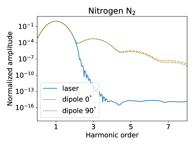
Figure 1: The spectral amplitude of the laser pulse and the induced dipole moment of an N₂ molecule for two molecular orientations. 0^∘ indicates that the polarization of the laser is aligned along the molecular axis, while for 90^∘ they are perpendicular.

The resulting magnitude of the dipole spectra at the fundamental laser frequency is found to have a $\cos^{2}(\theta)$ dependence even at a peak laser intensity of $I_{0}=10^{14}$ W/cm². Given the $\cos^{2}(\theta)$ dependence, it is possible to compute the polarization spectrum of an ensemble of randomly oriented molecules using a linear combination of the dipole spectra for parallel and perpendicular orientations of the molecules:

$$\hat{P}(\omega)=\rho\left(\frac{1}{3}\hat{d}_{\parallel}(\omega)+\frac{2}{3}\hat{d}_{\perp}(\omega)\right)\ ,$$ (2)

where $\rho$ is the neutral density of molecules. For N₂, $\rho=2.688\times 10^{25}$ m^-3 and for O₂ $\rho=2.505\times 10^{25}$ m^-3 at atmospheric pressure and room temperature. We note that this linear combination is typically valid only in the limit of low intensity laser pulses Boyd (2008). However, due to the low amount of ionization (a ground state population reduction of $\approx 10^{-5}$) that occurs for mid-infrared pulses even up to $10^{14}$ W/cm², we find that Eq. (2) is a good approximation.

The total susceptibility of the media, which includes both linear and nonlinear components, can be calculated by dividing the full polarization response spectrum $\hat{P}(\omega)$ by the laser’s spectrum $E(\omega)$:

$$\chi(\omega)=\frac{\hat{P}(\omega)}{\epsilon_{0}\hat{E}(\omega)}\ .$$ (3)

To extract the components of $\chi(\omega)$ corresponding to the linear $\chi^{(1)}(\omega)$ and nonlinear $\chi^{(3)}(\omega)$ properties of the medium, we employ a procedure that separates the linear and nonlinear responses spectrally.

In laser pulse propagation simulations the time-dependent polarization $P(t)$ of the medium is calculated as a power series expansion of odd harmonics of the field $E(t)$. For example, considering up to 5th order nonlinear processes, the polarization is

$$P(t)=\epsilon_{0}\left[\chi^{(1)}E(t)+\chi^{(3)}E^{3}(t)+\chi^{(5)}E^{5}(t)\right]\ .$$ (4)

We relate the expansion Eq. (4) to the various harmonics in the dipole spectrum using the Fourier transform, yielding a set of equations where each polarization spectra $\hat{P}(n\omega)$ can be written as a sum of linear and nonlinear contributions up to order $\chi^{(5)}$:

$$\frac{1}{\epsilon_{0}} \left[\hat{P}(\omega)+\hat{P}(3\omega)+\hat{P}(5\omega)\right]$$

$$=\chi^{(1)}\hat{E}_{1}(\omega)+\chi^{(3)}\hat{E}_{3}(\omega)+\chi^{(5)}\hat{E}_{5}(\omega)$$

$$+\cancel{\chi^{(1)}\hat{E}_{1}(3\omega)}+\chi^{(3)}\hat{E}_{3}(3\omega)+\chi^{(5)}\hat{E}_{5}(3\omega)$$

$$+\cancel{\chi^{(1)}\hat{E}_{1}(5\omega)}+\cancel{\chi^{(3)}\hat{E}_{3}(5\omega)}+\chi^{(5)}\hat{E}_{5}(5\omega)\ ,$$

where the quantities $\hat{E}_{n}(\omega)$ represent the Fourier transform of powers of the field $E^{n}(t)$. Terms containing no signal at a particular frequency are set to zero; for example there is no 3rd harmonic in the fundamental field and therefore $E_{1}(3\omega)=0$. Collecting terms of the same harmonic order yields a set of equations where each order susceptibility can be written in terms of the calculated molecular polarizations $P$ and field spectra $E$:

$$\chi^{(5)} =\frac{\hat{P}(5\omega)}{\epsilon_{0}\hat{E}_{5}(5\omega)}$$ (5)

$$\chi^{(3)} =\frac{\hat{P}(3\omega)}{\epsilon_{0}\hat{E}_{3}(3\omega)}-\chi^{(5)}\frac{\hat{E}_{5}(3\omega)}{\hat{E}_{3}(3\omega)}$$ (6)

$$\chi^{(1)} =\frac{\hat{P}(\omega)}{\epsilon_{0}\hat{E}_{1}(\omega)}-\chi^{(3)}\frac{\hat{E}_{3}(\omega)}{\hat{E}_{1}(\omega)}-\chi^{(5)}\frac{\hat{E}_{5}(\omega)}{\hat{E}_{1}(\omega)}$$ (7)

Conceptually, this corresponds to, for example, eliminating the contribution to the third harmonic yield from the fifth order process that involves absorbing four laser photons and emitting one, etc. The procedure is general and does not depend on the particular shape of the field $E(t)$. It also avoids division by small values since the polarization at each harmonic order is divided by a spectral field component that also contains a signal at that particular harmonic. However, we note that this perturbative approach is limited to intensity and wavelength regimes where ionization is small.

In practice, it is only necessary to consider nonlinear processes up to $\chi^{(5)}$ in order to extract intensity-independent values for $\chi^{(1)}$ and $\chi^{(3)}$. The magnitude of the nonlinear contribution to the fundamental and third harmonic polarizations drops off quite rapidly as the harmonic order increases and becomes negligible for harmonic orders 7 and above. We obtain intensity-independent susceptibilities over the wavelength range of $2-4$ $\mu$m for peak intensities up to $10^{14}$ W/cm². For wavelengths between $1-2$ $\mu$m, the extracted $\chi^{(3)}$ begins to show a small intensity dependence for peak intensity values above $5\times 10^{13}$ W/cm² due to a non-negligible amount of ionization. Intensity limitations of a perturbative approach of modeling the total susceptibility of a medium has also been observed in ab-initio calculations of atomic hydrogen Spott et al. (2014).

Using the expressions for susceptibility in Eqs. (5)-(7), the linear refractive index is

$$n_{0}(\omega)=\sqrt{1+\alpha\chi^{(1)}(\omega)}\ ,$$ (8)

where $\alpha$ is a scaling factor described in more detail below. The nonlinear refractive index is

$$n_{2}(\omega)=\frac{3}{4}\frac{\chi^{(3)}(\omega)}{\epsilon_{0}cn_{0}^{2}(\omega)}\ .$$ (9)

The scaling factor $\alpha$ ($\alpha=1.055$ for N₂ and $\alpha=1.034$ for O₂) is included to facilitate graphical comparison between the calculated values of this work and experimental values. The percentage adjustment of the linear susceptibility is consistent with the percentage difference between the calculated and measured values of $I_{p}$ for both species, $\Delta I_{p}^{\{\mathrm{N}_{2}\}}=3.9\%$ and $\Delta I_{p}^{\{\mathrm{O}_{2}\}}=5.7\%$, where the simulations have overestimated the binding energy of the highest energy electrons, resulting in a weaker response to the laser field.

IV Results

In Figure 2a, the calculated values of the linear index $n_{0}$ for N₂ are compared to the curve derived from experimental data (Peck and Khanna 1966 Peck and Khanna (1966))

$$n(\lambda)=1+6.497378\times 10^{-5}+\frac{3.0738649\times 10^{-2}}{\lambda_{0}^{-2}-\lambda^{-2}}\ ,$$ (10)

where $\lambda_{0}^{\{n_{0},\mathrm{N}_{2}\}}=0.0833$ $\mu$m and is valid from 0.4679 to 2.0586 $\mu$m. Despite the stated upper limit of 2 $\mu$m, Eq. (10) fits the calculated values remarkably well up to 4 $\mu$m. In Figure 2b, the nonlinear index is compared to experimental data (Zahedpour 2015 Zahedpour et al. (2015)) and is also found to be in very close agreement.

Since there is a decreasing spectral trend of the calculated values of $n_{2}$, it is interesting to compare its curve to the prediction provided by a generalized Miller’s rule for third order susceptibilities. Two formulations have been proposed in the literature. The first is $\chi^{(3)}(\omega)=\chi^{(3)}(\omega_{0})\left[\chi^{(1)}(\omega)/\chi^{(1)}(\omega_{0})\right]^{4}$ proposed by Ettoumi et al. Ettoumi et al. (2010) where $\omega_{0}$ corresponds to a reference value (e.g. 2 $\mu$m). The second is $\chi^{(3)}(\omega)=\delta\chi^{(1)}(3\omega)\chi^{(1)}(\omega)^{3}$ proposed by Bassani et al. Bassani and Lucarini (1998) where the factor $\delta=2.841\times 10^{-13}$ m²/V² is determined by performing a least-squares fit of the simulation data. In Figure 3, these predictive curves of $n_{2}$ are plotted along with the values calculated in this work.

It is clear that both predicted curves underestimate the dispersion of $n_{2}$ at long wavelengths compared to our calculated values, since both are “flatter” at long wavelengths. This finding is consistent with that of Ref. Mizrahi and Shelton (1985) which pointed out that Miller’s rule tends to underestimate the strength of the dispersion, and that there is not in general a strong correlation between the linear and nonlinear dispersion properties over a wide range of gases.

We find that the calculated values of $n_{2}$ are well fitted by a Sellmeier-like equation

$$n_{2}(\lambda)=\frac{P^{-1}}{\lambda_{0}^{-2}-\lambda^{-2}}\ ,$$ (11)

where $P^{\{\mathrm{N}_{2}\}}=14.63$ GW and $\lambda_{0}^{\{n_{2},N_{2}\}}=0.3334$ $\mu$m. As seen in Figure 3, Eq. (11) captures the dispersion of $n_{2}$ well, though it does force a singularity at $\lambda=0.333$ $\mu$m.

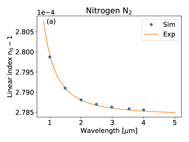
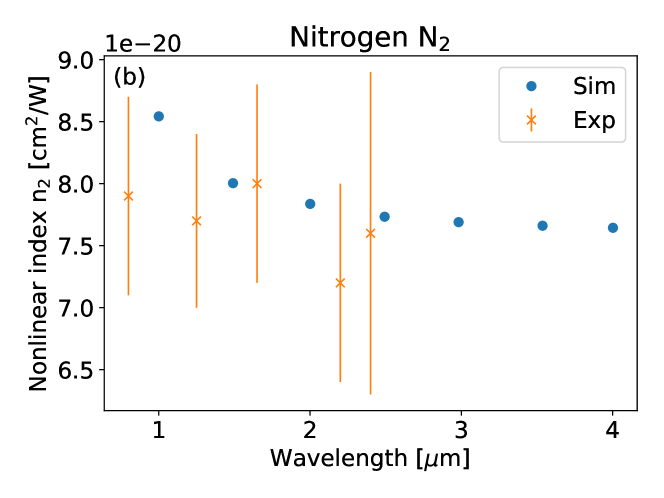
Figure 2: The calculated (Sim) optical properties of N₂ compared to experimental values (Exp). (a) The calculated index of refraction $n_{0}$ is compared to the curve Eq. (10). (b) The nonlinear refractive index $n_{2}$ compared to experimental data Zahedpour et al. (2015).

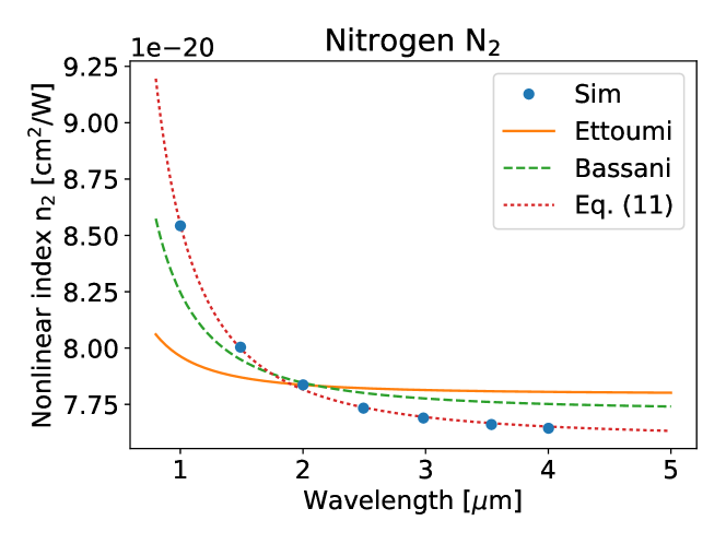
Figure 3: The calculated (Sim) nonlinear refractive index values $n_{2}$ of N₂ are compared to two formulations of a generalized Miller’s rule for third order susceptibilities. The best match for these values is obtained by a new Sellmeier-like equation Eq. (11).

In Figure 4, the calculated values for the linear index $n_{0}$ for O₂ are compared to the experimentally derived curve (Zhang 2008 Zhang et al. (2008), Kren 2011 Křen (2011))

$$n(\lambda)=1+1.181494\times 10^{-4}+\frac{9.708931\times 10^{-3}}{\lambda_{0}^{-2}-\lambda^{-2}}\ ,$$ (12)

where $\lambda_{0}^{\{n_{0},\mathrm{O}_{2}\}}=0.115$ $\mu$m and is valid from 0.4 to 1.8 $\mu$m. Extending this curve into the mid-infrared wavelength region shows that the scaled values of linear index from the simulation are well represented by Eq. (12).

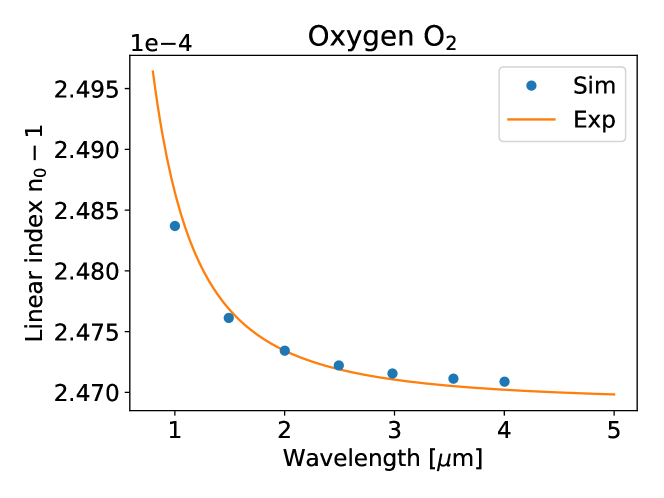
Figure 4: The calculated values (Sim) of the index of refraction $n_{0}$ of O₂ are compared to the experimentally derived curve Eq. (12) (Exp).

The calculated nonlinear index from the simulations are also in reasonable agreement with experimental data Zahedpour et al. (2015). However, we do not find an increase of $n_{2}$ near 2.4 $\mu$m which places our calculated values in closer agreement with the experimental data from Shelton and Rice Kaatz et al. (1998) for this particular wavelength. Just as with N₂, the values of $n_{2}$ for O₂ can be fitted with the Sellmeier-like equation Eq. (11) using the parameters $P^{\{\mathrm{O}_{2}\}}=14.62$ GW and $\lambda_{0}^{\{n_{2},\mathrm{O}_{2}\}}=0.3360$ $\mu$m.

We note that there is only a few percent difference between the calculated values of the nonlinear index n₂ for N₂ and O₂ and that this is merely a coincidence. In general, the value of $I_{p}$ for a particular species is not necessarily correlated with its value of $n_{2}$. A well-known example of this is the case of Ar and N₂ which have very similar values of $I_{p}$, yet $n_{2}$ for Ar is roughly 25% larger than that of N₂ in the MIR regime Zahedpour et al. (2015).

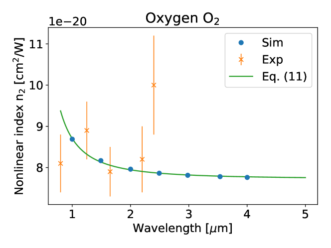
Figure 5: The calculated values (Sim) for the nonlinear refractive index $n_{2}$ of O₂ are compared to measured values Zahedpour et al. (2015) (Exp) and to Eq. (11) with the appropriate parameters.

A simple model for the optical properties of air can be constructed using a combination of the calculated susceptibilities for N₂ and O₂: $\chi^{(1)}_{air}=0.8\chi^{(1)}_{{\rm N}_{2}}+0.2\chi^{(1)}_{{\rm O}_{2}}$ and $\chi^{(3)}_{air}=0.8\chi^{(3)}_{{\rm N}_{2}}+0.2\chi^{(3)}_{{\rm O}_{2}}$. In Figure 6a, we compare the calculated values of $\chi^{(1)}_{air}$ to index curve Ciddor 1996 Ciddor (1996) (valid from $0.23-1.69$ $\mu$m) and index curves Mathar 2007 Mathar (2007) (valid in ranges $1.3-2.5$ $\mu$m and $2.8-4.2$ $\mu$m).

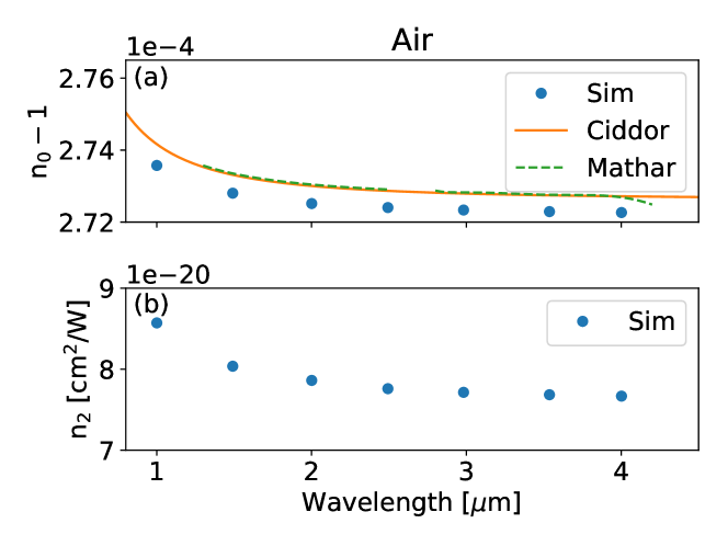
Figure 6: (a) The calculated linear index values for air (Sim) are compared to the linear index curves of Ciddor 1996 Ciddor (1996) and of Mathar 2007 Mathar (2007). (b) The nonlinear index values $n_{2}$ of air using a proportional combination of values from N₂ and O₂.

We find remarkably good agreement and therefore we can recommend the use of these curves for modeling the linear properties of air within the MIR wavelength regime of $1-4$ $\mu$m. In Figure 6b, we plot calculated values of the nonlinear index for air and recommend the use of these values in simulations of the propagation of MIR laser pulses.

V Summary

Using ab-initio calculations based on TDDFT, we have calculated the linear and nonlinear refractive indices for N₂, O₂, and air for wavelengths of $1-4$ $\mu$m. Close agreement between the experimental and calculated values of the linear index demonstrates that it is possible to extend the commonly-used linear index curves into the MIR region without modification. We also found that the calculated nonlinear index values $n_{2}$ for N₂ and O₂ are in good agreement with experimental values up to 2.4 $\mu$m, and our calculations provide new values for wavelengths up to 4 $\mu$m. We showed that the predictive formulas for the nonlinear index using Miller’s rule tend to underestimate the dispersion of $n_{2}$ at long wavelengths, and we proposed an empirical, Sellmeier-type, fit instead.

Our results show that a fully time-dependent calculation of the molecular response to a strong field can be used to reliably extract linear and nonlinear susceptibilities for intensities up to $5\times 10^{13}$ W/cm², as long as we correct for higher-order contributions to the dipole spectrum at a given frequency. Above $5\times 10^{13}$ W/cm² the ionization-induced depletion of the ground state starts to influence the calculation and the extracted susceptibilities are no longer intensity-independent. Our results provide a benchmark for future experimental and theoretical determination of the linear and nonlinear refractive indices in the MIR spectral range, and will allow for accurate calculations of phenomena involving long-distance propagation in air.

Acknowledgement: We acknowledge fruitful discussions with Paul Abanador, Ken Lopata and Ken Schafer. This material is based upon work supported by the Air Force Office of Scientific Research under MURI Award No. FA9550-16-1-0013.

References

- Couairon and Mysyrowicz (2007) A. Couairon and A. Mysyrowicz, Physics Reports 441, 47 (2007).
- Agostini and DiMauro (2008) P. Agostini and L. F. DiMauro, Contemporary Physics 49, 179 (2008), https://doi.org/10.1080/00107510802221630 .
- Panagiotopoulos et al. (2015) P. Panagiotopoulos, P. Whalen, M. Kolesik, and J. Moloney, Nature Photonics 9, 543 (2015).
- Peck and Khanna (1966) E. R. Peck and B. N. Khanna, J. Opt. Soc. Am. 56, 1059 (1966).
- Peck and Reeder (1972) E. R. Peck and K. Reeder, J. Opt. Soc. Am. 62, 958 (1972).
- Mizrahi and Shelton (1985) V. Mizrahi and D. P. Shelton, Phys. Rev. Lett. 55, 696 (1985).
- Ciddor (1996) P. E. Ciddor, Appl. Opt. 35, 1566 (1996).
- Zhang et al. (2008) J. Zhang, Z. H. Lu, and L. J. Wang, Appl. Opt. 47, 3143 (2008).
- Křen (2011) P. Křen, Appl. Opt. 50, 6484 (2011).
- Shelton and Rice (1994) D. P. Shelton and J. E. Rice, Chemical Reviews 94, 3 (1994), https://doi.org/10.1021/cr00025a001 .
- Zahedpour et al. (2015) S. Zahedpour, J. K. Wahlstrand, and H. M. Milchberg, Opt. Lett. 40, 5794 (2015).
- Mitrofanov et al. (2015) A. Mitrofanov, A. Voronin, D. Sidorov-Biryukov, A. Pugžlys, E. Stepanov, G. Andriukaitis, T. Flöry, S. Ališauskas, A. Fedotov, A. Baltuška, et al., Scientific reports 5 (2015), 10.1038/srep08368.
- Panov et al. (2016) N. A. Panov, D. E. Shipilo, V. A. Andreeva, O. G. Kosareva, A. M. Saletsky, H. Xu, and P. Polynkin, Phys. Rev. A 94, 041801 (2016).
- Bree et al. (2010) C. Bree, A. Demircan, and G. Steinmeyer, IEEE Journal of Quantum Electronics 46, 433 (2010).
- Brée et al. (2012) C. Brée, A. Demircan, and G. Steinmeyer, Phys. Rev. A 85, 033806 (2012).
- Tarazkar et al. (2016) M. Tarazkar, D. A. Romanov, and R. J. Levis, Phys. Rev. A 94, 012514 (2016).
- Tarazkar et al. (2015) M. Tarazkar, D. A. Romanov, and R. J. Levis, Journal of Physics B: Atomic, Molecular and Optical Physics 48, 094019 (2015).
- Andrade et al. (2015) X. Andrade, D. Strubbe, U. De Giovannini, A. H. Larsen, M. J. T. Oliveira, J. Alberdi-Rodriguez, A. Varas, I. Theophilou, N. Helbig, M. J. Verstraete, L. Stella, F. Nogueira, A. Aspuru-Guzik, A. Castro, M. A. L. Marques, and A. Rubio, Phys. Chem. Chem. Phys. 17, 31371 (2015).
- Andrade et al. (2012) X. Andrade, J. Alberdi-Rodriguez, D. A. Strubbe, M. J. T. Oliveira, F. Nogueira, A. Castro, J. Muguerza, A. Arruabarrena, S. G. Louie, A. Aspuru-Guzik, A. Rubio, and M. A. L. Marques, Journal of Physics: Condensed Matter 24, 233202 (2012).
- Krause et al. (1992) J. L. Krause, K. J. Schafer, and K. C. Kulander, Phys. Rev. A 45, 4998 (1992).
- Dirac (1930) P. A. M. Dirac, Mathematical Proceedings of the Cambridge Philosophical Society 26, 376–385 (1930).
- Bloch (1929) F. Bloch, Zeitschrift für Physik 57, 545 (1929).
- Perdew and Zunger (1981) J. P. Perdew and A. Zunger, Phys. Rev. B 23, 5048 (1981).
- Legrand et al. (2002) C. Legrand, E. Suraud, and P.-G. Reinhard, Journal of Physics B: Atomic, Molecular and Optical Physics 35, 1115 (2002).
- (25) “NIST electron-impact ionization cross sections,” https://physics.nist.gov/cgi-bin/Ionization/table.pl?ionization=N2.
- van Leeuwen and Baerends (1994) R. van Leeuwen and E. J. Baerends, Phys. Rev. A 49, 2421 (1994).
- Tognetti et al. (2008) V. Tognetti, P. Cortona, and C. Adamo, The Journal of Chemical Physics 128, 034101 (2008), https://doi.org/10.1063/1.2816137 .
- (28) “NIST electron-impact ionization cross sections,” https://physics.nist.gov/cgi-bin/Ionization/table.pl?ionization=O2.
- Boyd (2008) R. W. Boyd, in Nonlinear Optics (Third Edition), edited by R. W. Boyd (Academic Press, Burlington, 2008) third edition ed., pp. 253 – 275.
- Spott et al. (2014) A. Spott, A. Jaroń-Becker, and A. Becker, Phys. Rev. A 90, 013426 (2014).
- Ettoumi et al. (2010) W. Ettoumi, Y. Petit, J. Kasparian, and J.-P. Wolf, Opt. Express 18, 6613 (2010).
- Bassani and Lucarini (1998) F. Bassani and V. Lucarini, Il Nuovo Cimento D 20, 1117 (1998).
- Kaatz et al. (1998) P. Kaatz, E. A. Donley, and D. P. Shelton, The Journal of Chemical Physics 108, 849 (1998), https://doi.org/10.1063/1.475448 .
- Mathar (2007) R. J. Mathar, Journal of Optics A: Pure and Applied Optics 9, 470 (2007).