Better than Rician: Modelling millimetre wave channels as Two-Wave with Diffuse Power

Abstract

This contribution provides experimental evidence for the two-wave with diffuse power (TWDP) fading model. We have conducted two indoor millimetre wave measurement campaigns with directive horn antennas at both link ends. One horn antenna is mounted in a corner of our laboratory, while the other is steerable and scans azimuth and elevation. Our first measurement campaign is based on scalar network analysis with $7$ GHz of bandwidth. Our second measurement campaign obtains magnitude and phase information, additionally sampled directionally at several positions in space. We apply Akaike’s information criterion to decide whether Rician fading sufficiently explains the data or the generalized TWDP fading model is necessary. Our results indicate that the TWDP fading hypothesis is favoured over Rician fading in situations where the steerable antenna is pointing towards reflecting objects or is slightly misaligned at line-of-sight. We demonstrate TWDP fading in several different domains, namely, frequency, space, and time.

1 Introduction

Accurate modelling of wireless propagation effects is a fundamental prerequisite for a proper communication system design. After the introduction of the double-directional radio channel model [1], wireless propagation research ($<6$ GHz) started to model the wireless channel agnostic to the antennas used. More than a decade later, propagation research focusses now on millimetre wave bands to unlock the large bandwidths available in this regime [2, 3, 4, 5]. At millimetre waves, omnidirectional antennas have small effective antenna areas, resulting in a high path-loss [6, 7, 8, 9, 10]. To overcome this high path-loss, researchers have proposed to apply highly directive antennas on both link ends [11, 12, 13, 14]. Most researchers aim to achieve high directivity with antenna arrays [15, 16, 17, 18, 19, 20] and a few with dielectric lenses [21, 22, 23]. When the link-quality depends so much on the achieved beam-forming gain, antennas must be considered as part of the wireless channel again. Small-scale fading is then influenced by the antenna.

According to Durgin [24, p. 137], “The use of directive antennas or arrays at a receiver, for example, amplifies several of the strongest multipath waves that arrive in one particular direction while attenuating the remaining waves. This effectively increases the ratio of specular to nonspecular received power, turning a Rayleigh or Rician fading channel into a TWDP fading channel.” The mentioned two-wave with diffuse power (TWDP) fading channel describes this spatial filtering effect by two non-fluctuating receive signals together with many smaller diffuse components.

1.1 Related work

The authors of [25] investigated a simple wall scattering scenario and analysed how fading scales with various antenna directivities and different bandwidths. Increasing directivity [25], as well as increasing bandwidth [25, 26], results in an increased Rician K-factor. The authors of [27] analysed fading at $28$ GHz with high gain horn antennas on both link ends. They observe high Rician K-factors even at non-line-of-sight (NLOS). This effect is explained by spatial filtering of directive antennas, as they suppress many multipath components [25]. Outdoor measurements in [28, 29], show a graphical agreement with the Rice fit, but especially Fig. 10 in [29] might be better explained as TWDP fading.

TWDP fading has already successfully been applied to describe $60$ GHz near body shadowing [30]. Furthermore, as quoted above, TWDP must be considered for arrays, as they act as spatial filters [31, 24]. While theoretical work on TWDP fading is already advanced [32, 33, 34, 35, 36, 37, 38], experimental evidence, especially at millimetre waves, is still limited. For enclosed structures, such as aircraft cabins and buses, the applicability of the TWDP model is demonstrated by Frolik [39, 40, 41, 42, 43]. A deterministic two ray behaviour in ray tracing data of mmWave train-to-infrastructure communications is shown in [44]. A further extension of the TWDP-fading model, the so called fluctuating two-ray fading model, was also successfully applied to fit mmWave measurement data [36].

Our group has conducted two measurement campaigns [45, 46] to directionally analyse receive power and small-scale fading parameters for mmWaves. This contribution is based on [45, 46].

1.2 Outline and contributions

With this contribution, we aim to bring scientific rigour to the small-scale fading analysis of millimetre wave indoor channels. We show in Section 2 – by means of an information-theoretic approach [47] and null hypothesis testing [48] – that the TWDP model has evidence in mmWave communications.

We have conducted two measurement campaigns within the same laboratory with different channel sounding concepts. Our measurements are carried out in the V-band; the applied center frequency is $60$ GHz. For both measurement campaigns, $20$ dBi horn antennas are used at the transmitter and at the receiver. The first measurement campaign (MC1) samples the channel in azimuth ($\varphi$) and elevation ($\theta$), keeping the antenna’s (apparent) phase center [49, pp. 799] at a fixed $(x,y)$ – coordinate. The transmitter is mounted in a corner of our laboratory. The sounded environment as well as the mechanical set-ups are explained in Section 3. For MC1, we sounded the channel in the frequency-domain by aid of scalar network analysis, described in Section 4. These channel measurements span over $7$ GHz bandwidth, supporting us to analyse fading in the frequency domain.

For the second measurement campaign (MC2), described in Section 5, we improved the set-up mechanically and radio frequency (RF) – wise. By adding another linear guide along the $z$-axis, we keep the antenna’s phase center constant in $(x,y,z)$ – coordinate, irrespective of the antenna’s elevation. Furthermore, we changed the sounding concept to time-domain channel sounding. This approach allows us to utilise the time domain and to show channel impulse responses in Section 7. Additionally, by adjusting $(x,y,z,\varphi,\theta)$, we sample the channel in the spatial domain at all directions $(\varphi,\theta)$. These improvements enable us to show spatial correlations in Section 6, a further analysis tool to support the claims from MC1.

In summary, we demonstrate TWDP fading for directional mmWave indoor channels in the frequency-domain, in the spatial-domain, and in the time-domain.

2 Methodology - Fading model identification

TWDP fading captures the effect of interference of two non-fluctuating radio signals and many smaller so called diffuse signals [31]. The TWDP distribution degenerates to Rice if one of the two non-fluctuating radio signals vanishes. This is analogous to the well known Rice degeneration to the Rayleigh distribution with decreasing K factor. In the framework of model selection, TWDP fading, Rician fading, and Rayleigh fading are hence nested hypotheses [47]. Therefore, it is also obvious that among these alternatives, TWDP always allows the best possible fit of measurement data. Occam’s razor [50] asks to select, among competing hypothetical distributions, the hypothesis that makes the fewest assumptions. Different distribution functions are often compared via a goodness-of-fit test [51]. Nevertheless, the authors of [52] argue that Akaike’s information criterion (AIC) [53, 54, 55, 47] is better suited for the purpose of choosing among fading distributions. Later on, the AIC was also used in [56, 57, 58, 59, 60]. The AIC can be seen as a form of Occam’s razor as it penalizes the number of estimable parameters in the approximating model [47] and hence aims for parsimony.

2.1 Mathematical description of TWDP fading

An early form of TWDP was analysed in [32]. Durgin et al. [31] introduced a random phase superposition formalism. Later, [35] achieved a major breakthrough and found a description of TWDP fading as conditional Rician fading. For the benefit of the reader, we will briefly repeat some important steps of [35].

The TWDP fading model in the complex-valued baseband is given as

$$r_{\text{complex}}=V_{1}e^{j\phi_{1}}+V_{2}e^{j\phi_{2}}+X+jY~{},$$ (1)

where $V_{1}\geq 0$ and $V_{2}\geq 0$ are the deterministic amplitudes of the non-fluctuating specular components. The phases $\phi_{1}$ and $\phi_{2}$ are independent and uniformly distributed in $(0,2\pi)$. The diffuse components are modelled via the law of large numbers as $X+jY$, where $X,Y\sim\mathcal{N}(0,\sigma^{2})$. The $K$-factor is the power ratio of the specular components to the diffuse components

$$K=\frac{V_{1}^{2}+V_{2}^{2}}{2\sigma^{2}}~{}.$$ (2)

The parameter $\Delta$ describes the amplitude relationship among the specular components

$$\Delta=\frac{2V_{1}V_{2}}{V_{1}^{2}+V_{2}^{2}}~{}.$$ (3)

The $\Delta$-parameter is bounded between $0$ and $1$ and equals $1$ iff both amplitudes are equal. The second moment of the envelope $r=|r_{\text{complex}}|$ of TWDP fading is given as

$$\mathbb{E}\big{[}r^{2}\big{]}=\Omega=V_{1}^{2}+V_{2}^{2}+2\sigma^{2}~{}.$$ (4)

Expectation is denoted by $\mathbb{E}$. For bounded amplitudes $V_{1}$ and $V_{2}$, a clever choice of $\sigma^{2}$ normalises $\Omega$, that is $\Omega\equiv 1$. Starting from (4), by using (2) we arrive at

$$\sigma^{2}=\frac{1}{2(1+K)}~{}.$$ (5)

Given the $K$ and $\Delta$ parameter ($\Omega\equiv 1$), the authors of [61] provide a formula for the amplitudes of both specular components

$$V_{1,2} =\frac{1}{2}\sqrt{\frac{K}{K+1}}\big{(}\sqrt{1+\Delta}\pm\sqrt{1-\Delta}\big{)}~{}.$$ (6)

Real-world measurement data have $\Omega\neq 1$. To work with the formalism introduced above, we normalise the measurement data through estimating $\hat{\Omega}$ by the method of moments. The second moment $\Omega$ of Rician fading and TWDP fading is merely a scale factor [62, 63]. Notably, we are more concerned with a proper fit of $K$ and $\Delta$. Generally, estimation errors on $\Omega$ propagate to $K$ and $\Delta$ estimates. However, [62] achieved an almost asymptotically efficient estimator with a moment-based estimation of $\Omega$.

Our envelope measurements are partitioned into 2 sets. We take the first set ($r_{1},\ldots,r_{n},\ldots r_{N}$) for parameter estimation of the tuple ($K,\Delta$) as described in Section 2.2, and hypothesis testing as described in Section 2.3. The first set is carefully chosen to obtain envelope samples that are approximately independent and identically distributed. The second set ($r_{1},\ldots,r_{m},\ldots r_{M}$) is the complement of the first set. We use the elements of the second set to estimate the second moment via

$$\hat{\Omega}=\frac{1}{M}\sum\limits_{m=1}^{M}r_{m}^{2}~{},$$ (7)

where $m$ is the sample index and $M$ is the size of the second set. Partitioning is necessary to avoid biases through noise correlations of $\hat{\Omega}$ and ($\hat{K},\hat{\Delta}$) [64].

By considering the estimate (7) as true parameter $\Omega$, all distributions are parametrised by the tuple ($K,\Delta$), solely. Example distributions are shown in Fig. 1. The cumulative distribution function (CDF) of the envelope of (1) is given in [35] as

$$F_{\text{TWDP}}(r;K,\Delta)=$$ (8)

$$1-\frac{1}{2\pi}\int\limits_{0}^{2\pi}Q_{1}\!\! \left(\sqrt{2K\left[1+\Delta\cos\left(\alpha\right)\right]},\frac{r}{\sigma}\right)\text{d}\alpha~{}.$$

The Marcum Q-function is denoted by $Q_{1}(\cdot,\cdot)$. For $\Delta\rightarrow 0$, Equation (8) reduces to the well known Rice CDF

$$F_{\text{Rice}}(r;K)=1-Q_{1}\left(\sqrt{2K},\frac{r}{\sigma}\right)~{}.$$ (9)

It might sound tempting to have a second strong radio signal present; in fact, however, two waves can either superpose constructively or destructively and eventually lead to fading that is more severe than Rayleigh [39, 40, 41, 42, 43]. We observe the highest probability for deep fades for TWDP fading in Fig. 1.

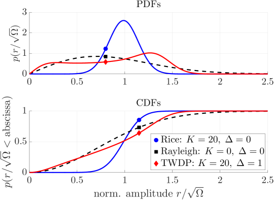
Figure 1: Comparison of Rayleigh, Rician, and TWDP fading. The TWDP distribution with $\Delta=1$ deviates from the Rice distribution. TWDP fading’s probability for deep fades is higher than for a Rayleigh distribution.

2.2 Parameter estimation and model selection

Note that our model of TWDP fading (1) does (obviously) not contain noise. Over our wide frequency range (in MC1 we have $7$ GHz bandwidth) the receive noise power spectral density is not equal. A statistical noise description that is valid over our wide frequency range is frequency-dependent. To avoid the burden of frequency-dependent noise modelling, we only take measurement samples which lie at least $10$ dB above the noise power and ignore noise in our estimation.

Having the envelope measurement data set ($r_{1},\ldots,r_{n},\ldots r_{N}$) at hand, we are seeking a distribution of which the observed realisations $r_{n}$ appear most likely. To do so, we estimate the parameter tuple ($K$,$\Delta$) via the maximum likelihood procedure

$$(\hat{K},\hat{\Delta}) =\operatorname*{arg\,max}_{K,\Delta}\sum_{n=1}^{N}\operatorname{ln}\frac{\partial F_{\text{TWDP}}(r_{n};K,\Delta)}{\partial r}$$

$$=\operatorname*{arg\,max}_{K,\Delta}\sum_{n=1}^{N}\operatorname{ln}f_{\text{TWDP}}(r_{n};K,\Delta)$$

$$=\operatorname*{arg\,max}_{K,\Delta}\sum_{n=1}^{N}\operatorname{ln}\mathcal{L}(K,\Delta|r_{n})~{}.$$ (10)

We denote the probability density function (PDF) by $f(\cdot)$, $n$ denotes the sample index, and $N$ the size of the set. To solve (10), we first discretise $K$ and $\Delta$ in steps of $0.05$. Next, we calculate $\frac{\partial F_{\text{TWDP}}(r;K,\Delta)}{\partial r}$ for all parameters via numerical differentiation. Within this family of distributions, we search for the parameter vector maximizing the log-likelihood function (10). For the optimal Rice fit, the maximum is searched within the parameter slice ($K,\Delta=0$). An exemplary fit of Rician and TWDP fading is shown in Fig. 2. As a reference, Rayleigh fading ($K=0,\;\Delta=0$) is shown as well.

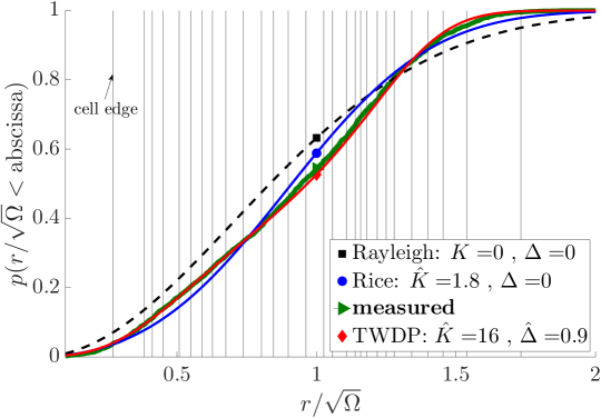
Figure 2: CDF: Distribution fitting for exemplary frequency domain measurement data. Illustration of the maximum likelihood fitted Rice distribution and the maximum likelihood fitted TWDP fading distribution. The Rician $K$-factor and the TWDP $K$-factor deviate significantly. Rayleigh fading is plotted as reference.

To select between Rician fading and TWDP fading, we employ Akaike’s information criterion (AIC). The AIC is a rigorous way to estimate the Kullback–Leibler divergence, that is, the relative entropy based on the maximum-likelihood estimate [47]. Given the maximum-likelihood fitted parameter tuple ($\hat{K},\hat{\Delta}$) of TWDP fading and Rician fading, we calculate the sample size corrected AIC [47, p. 66] for Rician fading ($\text{AIC}_{\text{R}}$) or TWDP fading ($\text{AIC}_{\text{T}}$)

$$\text{AIC}_{\text{R/T}}=$$ (11)

$$-2\operatorname{ln}\mathcal{L}_{\text{R/T}}(\hat{K},\hat{\Delta}|r)+2U_{\text{R/T}}+\frac{2U_{\text{R/T}}(U_{\text{R/T}}+1)}{N-U_{\text{R/T}}-1}~{},$$

where $U$ is the model order. For Rician fading the model order is $U_{\text{R}}=1$, since we estimate the $K$-factor, only. For TWDP fading $U_{\text{T}}=2$, as $\Delta$ is estimated additionally. The second moment $\Omega$ (estimated already with a different data set before the parameter estimation) is not part of the ML estimation (10) and therefore not accounted in the model order $U$. We choose between Rician fading and TWDP fading based on the lower AIC.

2.3 Validation of the chosen model

Based on (11), one of the two distributions, Rice or TWDP, will always yield a better fit. To validate whether the chosen distributions really explains the data, we state the following statistical hypothesis testing problem:

$$\mathcal{H}_{0}: \begin{cases}F_{\text{Rice}}(r;\hat{K}),&\text{if }\text{AIC}_{\text{R}}\leq\text{AIC}_{\text{T}}\\ F_{\text{TWDP}}(r;\hat{K},\hat{\Delta}),&\text{else}\end{cases}$$

$$\mathcal{H}_{1}: \begin{cases}\neg F_{\text{Rice}}(r;\hat{K}),&\text{if }\text{AIC}_{\text{R}}\leq\text{AIC}_{\text{T}}\\ \neg F_{\text{TWDP}}(r;\hat{K},\hat{\Delta}),&\text{else}\end{cases}$$ (12)

The Boolean negation is denoted by $\neg$. Our statistical tool is the g-test [65, 66]. At a significance level $\alpha$, a null hypothesis is rejected if

$$G=2\sum_{i=1}^{m}O_{i}\ln\bigg{(}\frac{O_{i}}{E_{i}}\bigg{)}\overset{\mathbf{?}}{>}\chi_{(1-\alpha,m-e)}^{2}~{},$$ (13)

where $O_{i}$ is the observed bin count in cell $i$ and $E_{i}$ is the expected bin count in cell $i$ under the null hypothesis $\mathcal{H}_{0}$. The cell edges are illustrated with vertical lines in Fig. 2. The cell edges are chosen, such that $10$ observed bin counts fall into one cell. The estimated parameters of the model are denoted by $e$. For Rician fading we estimate $e=2$ ($\Omega,K$) parameters and for TWDP fading we estimate $e=3$ ($\Omega,K,\Delta$) parameters in total. The $(1-\alpha)$ – quantile of the chi-square distribution with $m-e$ degrees of freedom is denoted by $\chi_{(1-\alpha,m-e)}^{2}$. The prescribed confidence level is $1-\alpha=0.01$ .

3 Floor plan and set-ups for MC1 and MC2

Our measured environment is a mixed office and laboratory room. There are office desks in the middle of the room and at the window side, there are laboratory desks, see Fig 3. The main interacting objects in our channel are office desks, a metallic fridge, a wall, and the surface of the laboratory desk. These objects are all marked in Fig. 3.

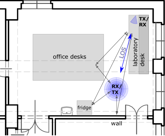
Figure 3: Floor plan of the measured environment. The floorplan indicates the multipath components that are visible in the measurement results. TX and RX switch roles for MC2. TX/RX in the right upper corner of the room is always static. RX/TX in the middle of the room is steerable, indicated by the spider’s web.

Our directional measurements are carried out by using the traditional approach of mechanically steered directional antennas [68, 69]. As directional antennas, $20$ dBi conical horn antennas with an $18^{\circ}$ $3$ dB opening angle are used. Our polarisation is determined by the LOS polarisation. When TX and RX are facing each other at LOS, the polarisation is co-polarised and the E-field is orthogonal to the floor. In MC1, the essential mechanical adaptation to the state-of-the-art directional channel sounding set-up [70, 71] is that the elevation-over-azimuth positioner is mounted on an xy-positioning stage. Thereby, we compensate for all linear translations caused by rotations and keep the phase center of the horn antenna always at the same $(x,y)$ coordinate, see Fig. 4. The $z$ coordinate is roughly $70$ cm above ground but varies $13$ cm for different elevation angles.

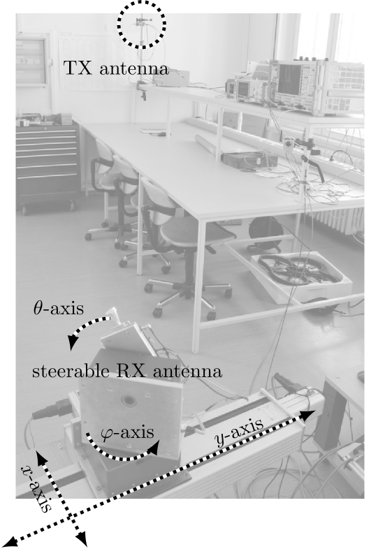
Figure 4: Photograph of the mechanical set-up for MC1 from the receiver point of view. The receive antenna, a conical $20$ dBi horn, is mounted on a multi-axis positioning and rotating system. The azimuthal and elevation angle are controlled to scan the whole upper hemisphere. The multi-axis system moves and rotates the horn antenna such that its phase center stays at the same $(x,y)$ coordinate during the directional scan.

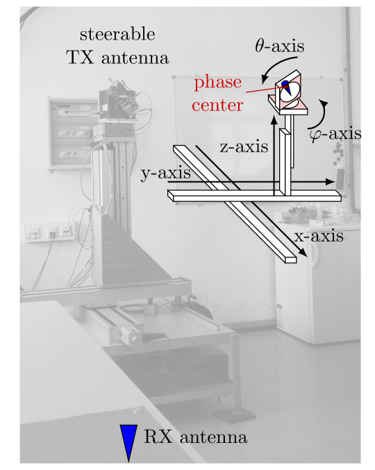
Figure 8: Photograph of the improved mechanical set-up for MC2 from the receiver point of view. Our mechanical set-up consists now of five independent axis to fully compensate all offsets introduced by rotation. A schematic sketch is superimposed. All five axis are necessary to rotate the horn antenna around the phase center at a fixed $(x,y,z)$ coordinate. Notice that TX and RX switch roles as compared to Fig. 4.

For MC2 we add another linear guide along the $z$-axis to compensate for all introduced offsets. The horn antenna’s phase center is thereby lifted upwards by one metre. Now we are able to fix the phase center of the horn antenna at a specific $(x,y,z)$ coordinate in space. The whole mechanical set-up and the fixed phase center is illustrated in Fig. 8.

4 MC1: Scalar-valued wideband measurements

A wireless channel is said to be small-scale fading, if the receiver (RX) cannot distinguish between different multipath components. Depending on the position of the transmitter (TX), the position of the RX and the position of the interacting components, the MPCs interfere constructively or destructively [72, pp. 27]. The fading concept only asks for a single carrier frequency, whose MPCs arrive with different phases at the RX. By spatial sampling a statistical description of the fading process is found.

In MC1, the spatial $(x,y)$ – coordinate (of TX and RX) is kept constant. Different phases of the impinging MPCs are realised by changing the TX frequency over a bandwidth of $7$ GHz. Thereby we implicitly rely on frequency translations to estimate the moments of the spatial fading process.

4.1 Measurement set-up

We measure the forward transfer function with an Rohde and Schwarz R&S ZVA24 vector network analyser (VNA). The VNA can measure directly up to $24$ GHz. For mmWave up-conversion and down-conversion, we employ modules from Pasternack [73]. They are based on radio frequency integrated circuits described in [74]. The up-converter module and the down-converter module are operating built-in synthesizer phase-locked loops, where the local oscillator (LO) frequency is calculated as

$$f_{\text{LO}}=\nicefrac{{7}}{{4}}\cdot s_{\text{PLL}}\cdot 285.714\,\text{MHz}\approx s_{\text{PLL}}\cdot 500\,\text{MHz}~{}.$$ (14)

The scaling factor of the synthesizer PLL counters is denoted by $s_{\text{PLL}}$. For $f_{\text{LO}}\approx 60\,\text{GHz}$, the scaling factor is $s_{\text{PLL}}=120$. To avoid crosstalk, we measure the transfer function via the conversion gain (mixer) measurement option of our VNA and operate the transmitter and receiver at different baseband frequencies: $601$ to $1100$ MHz and $101$ to $600$ MHz. The set-up is shown in Fig. 5.

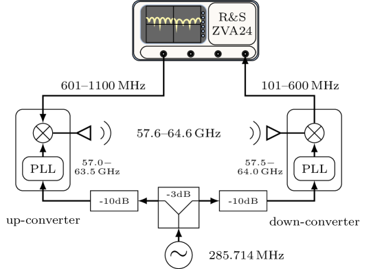
Figure 5: RF set-up for MC1. The combination of different PLL scaling factors allows for a measurement bandwidth of $7$ GHz. The reference clock for the up-converter and the down-converter is shared. The power splitter has an isolation of $30$ dB. To avoid possible leakage on the clock distribution network, attenuators additionally decouple both converters. The transfer function is measured applying the conversion gain (mixer) measurement option of the R&S VNA.

4.2 Receive power and fading distributions

In Fig. 6, we show the estimated received mean power of $7$ GHz bandwidth, normalised to the maximum RX power, that is

$$P_{\text{RX,norm.}}(\varphi,\theta)=\frac{\hat{\Omega}(\varphi,\theta)}{\max_{\varphi^{\prime},\theta^{\prime}}(\hat{\Omega}(\varphi^{\prime},\theta^{\prime}))}~{}.$$ (15)

As already mentioned in Section 2, we partition the frequency measurements into two sets. The normalised receive power is calculated according to (7), with frequency samples spaced by $2.5$ MHz. Every tenth sample is left out as these samples are used for fitting of ($K,\Delta$) and hypothesis testing. We display the results via a stereographic projection from the south pole and use $\tan(\nicefrac{{\theta}}{{2}})$ as azimuthal projection. All samplings points, lying at least $10$ dB above the noise level, are subject of our study. They are displayed with red, white or black markers. Sampling points where we decided for TWDP fading, following the procedure described in Section 2, are marked with red diamonds. White circles mark points for which AIC favours Rician fading. Four points are marked black. These points failed the null hypothesis test and we neither argue for Rician fading nor for TWDP fading. TWDP fading occurs whenever the line-of-sight (LOS)-link is not perfectly aligned or if the interacting object cannot be described by a pure reflection.

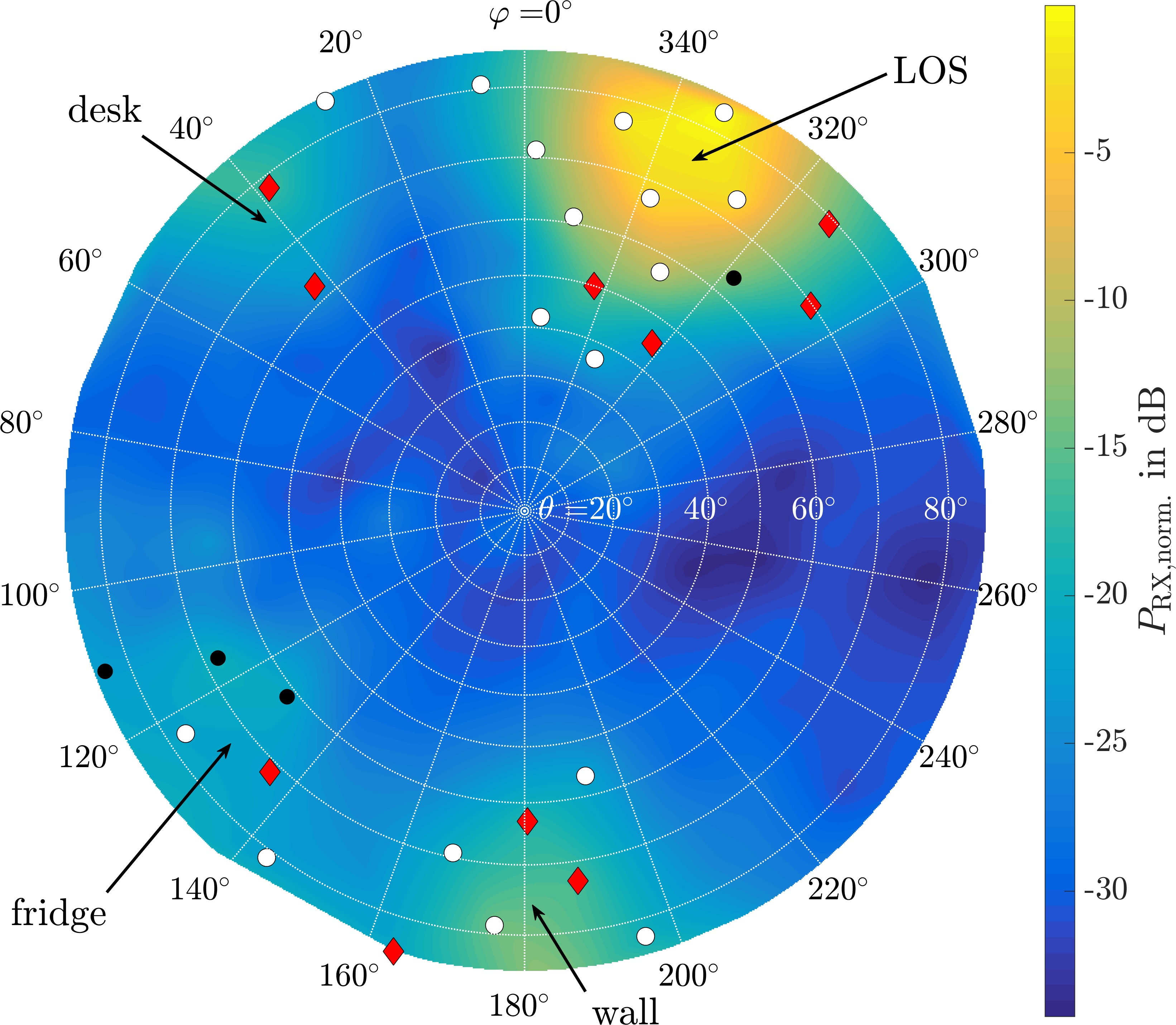
Figure 6: Estimated directional receive power of MC1. There are four main interacting objects leading to stronger receive power (marked in the figure). TWDP fading occurs whenever the LOS-link is not perfectly aligned or the reflecting structure is not perfectly plain. Red diamonds mark TWDP fading and white circles mark Rician fading. Black markers show points where both distributions are rejected by the hypothesis test. Directions less than $10$ dB above the noise level are not evaluated.

In Fig. 7, the $K$-parameter of the selected hypothesis is illustrated. Figure 7 shows either the Rician K-factor or the TWDP K-factor, depending on the selected hypothesis. Note that their definitions are fully equivalent. For Rician fading, the amplitude $V_{2}$ in (1) is zero by definition. Whenever the RX power is high, the $K$-factor is high. Below the $K$-estimate, the estimate of $\Delta$ is shown. Here again, by definition, $\Delta=0$ whenever we decide for Rician fading. For interacting objects, the parameter $\Delta$ tends to be close to one. Note, that decisions based on AIC select TWDP fading mostly when $\Delta$ is above $0.3$. Smaller $\Delta$ values do not change the distribution function sufficiently to justify a higher model order.

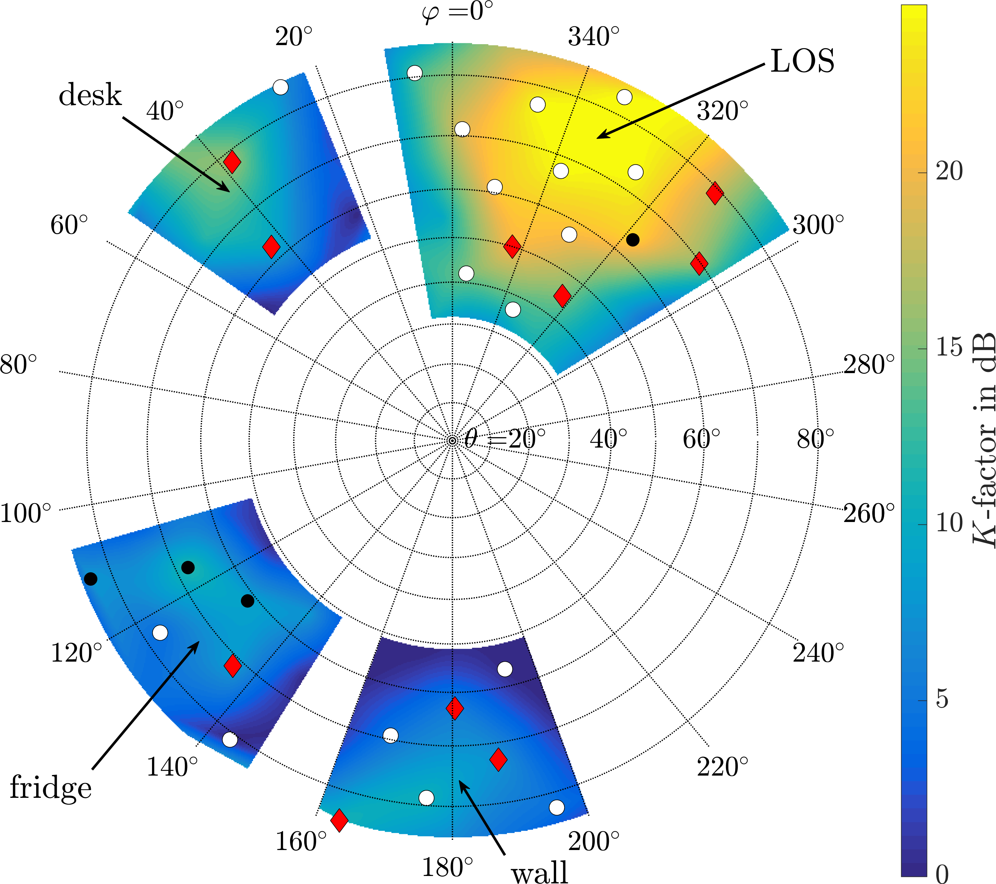
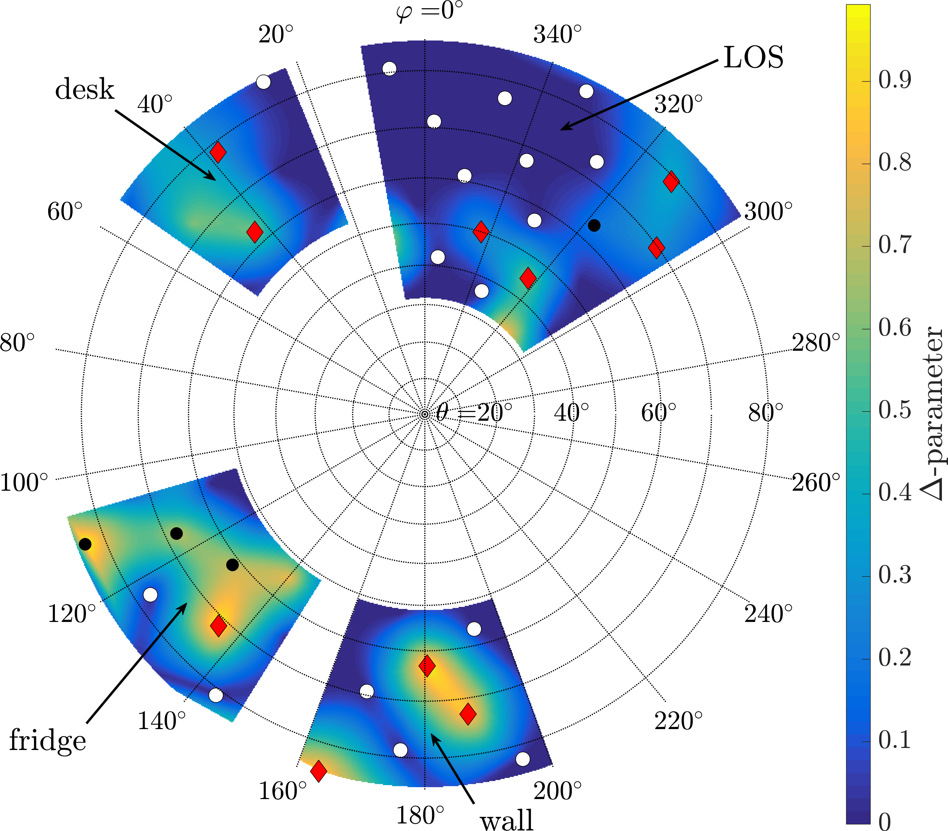
Figure 7: Estimated $K$-factor and $\Delta$-parameter of MC1. We plot the $K$-factor estimate of the selected hypothesis. The $K$-factor behaves analogously to the RX power. At LOS, the $K$-factor is far above $20$ dB. The desk reflection has a surprisingly high $K$-factor of about $15$ dB. Other reflections have $K$-factors of approximately $10$ dB. The $\Delta$-parameter for reflections tends to be close to $1$. Markers have the same meaning as in Fig. 6.

5 MC2: Vector-valued spatial measurements

In contrast to MC1, we no longer rely on frequency translations and are indeed sampling the channel in space. The fading results we present in Section 5.3 are evaluated at a single frequency. Fading is hence determined by the obtained spatial samples, exclusively.

5.1 Measurement set-up

At the transmitter side, a $2$ GHz wide waveform is produced by an arbitrary waveform generator (AWG). A multi-tone waveform (OFDM) with Newman phases [75, 76, 77] is applied as sounding signal. The signal has $401$ tones (sub-carriers) with a spacing of $5$ MHz. This large spacing assures that our system is not limited by phase noise [78]. The TX sequence is repeated $2\,000$ times to obtain a coherent processing gain of $33$ dB for i.i.d. noise. The Pasternack up-converter (the same as in MC1) shifts the baseband sequence to $60$ GHz. The $20$ dBi conical horn antenna, together with the up-converter is mounted on a five axis positioner to directionally steer them. As receiver, a signal analyser (SA) (R&S FSW67) with a 2 GHz analysis bandwidth is used. The received in-phase and quadrature (IQ) baseband samples are obtained from the SA. The whole system is sketched in Fig. 9.

In MC2, for feasibility reasons, TX and RX switch places compared to MC1. The RX in form of the SA is put onto the laboratory table. The RX $20$ dBi conical horn antenna is directly mounted at the RF input of the SA. The SA is located on a table close to a corner of the room; the RX antenna is not steered.

Similar to the set-ups of [79, 80, 81, 82], proper triggering between the arbitrary waveform generator and the SA ensures a stable phase between subsequent measurements.

Figure 9: RF set-up for MC2. The VNA from Fig. 5 is replaced with an AWG and an SA. This leads to a set-up where we obtain phase information as well. An option of the SA gives us direct access to the baseband IQ samples.

5.2 Receive power

For the calculation of the RX power, averaged over $2$ GHz bandwidth, we perform a sweep through azimuth and elevation at a single coordinate. The LOS and wall reflection from MC1 are still visible in Fig. 10. Fading is evaluated at a single frequency in the subsection below. Nevertheless, we already indicate fading distributions by markers in Fig. 10 in order to better orient ourselves later on.

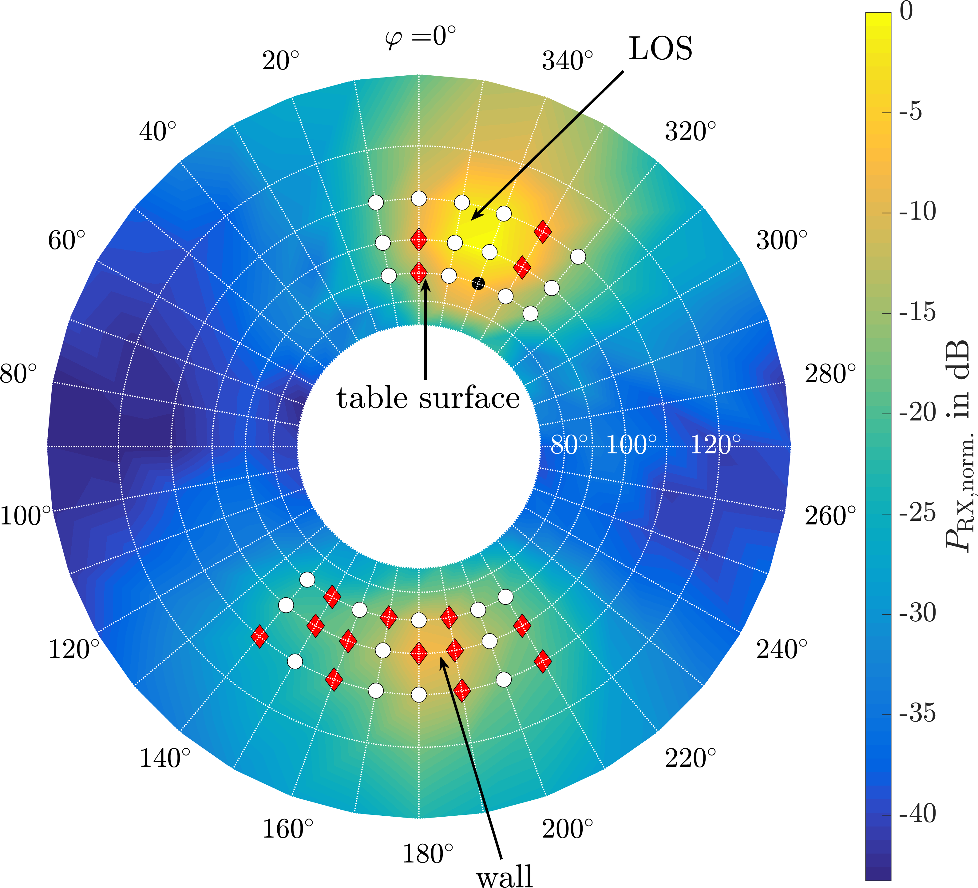
Figure 10: Estimated directional receive power of MC2. Due to the elevated position of the steerable horn antenna, two interacting objects from Fig. 6, namely the desk and the fridge, are no longer visible. LOS and the wall reflection are still present. These regions are the only ones which are spatially sampled. Markers have the same meaning as in Fig. 6.

As the steerable horn antenna is above the office desks and the fridge level, these interacting objects do not become apparent. In case the steerable TX does not hit the RX at LOS accurately, the table surface acts as reflector and a TWDP model explains the data. For wall reflections, with non-ideal alignment, TWDP also explains the data best.

5.3 Fading distributions

To obtain different spatial realisations, with the horn antenna pointing into the same direction, the coordinate of the apparent phase center is moved to ($x,y,z$) – positions uniformly distributed within a cube of side length $2.8\lambda$, see Fig. 11. We realise a set of $9\times 9\times 9=729$ directional measurements. This results in a spacing between spatial samples of $0.35\lambda$ in each direction. Although $\nicefrac{{\lambda}}{{2}}$ sampling is quite common [25, 27], we choose the sampling frequency to be co-prime with the wavelength, to circumvent periodic effects [83]. We restrict our spatial extend to avoid changes in large-scale fading. Only at directions with strong reception levels do we perform spatial sampling. Similar as in the previous section, we partition the measurements into 2 sets. The partitioning is made according to a 3D chequerboard pattern. The first set is used for the estimation of the second moment $\hat{\Omega}$ and the second set is used for the parameter tuple ($K,\Delta$).

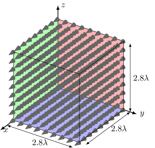
Figure 11: Spatial sampling grid. For one specific direction, we draw $9\times 9\times 9=729$ samples uniformly from a cube of side length $2.8\lambda$. The distance between samples is $0.35\lambda$ with a repeat accuracy of $\pm 0.004\lambda$. The orientation of the horn antenna is indicated via the cone shape at the sampling points.

The best fitting $K$-factors, in both regions with strong reception, are illustrated in Fig. 12, top part. Below the $\Delta$-parameters are provided. Remember, the RX in form of an SA is put on the laboratory table. In case the TX is not perfectly aligned, a reflection from the table surface yields a fading statistic captured by the TWDP model. The interaction with the wall, similar to Fig. 7, has again regions best modelled via TWDP fading.

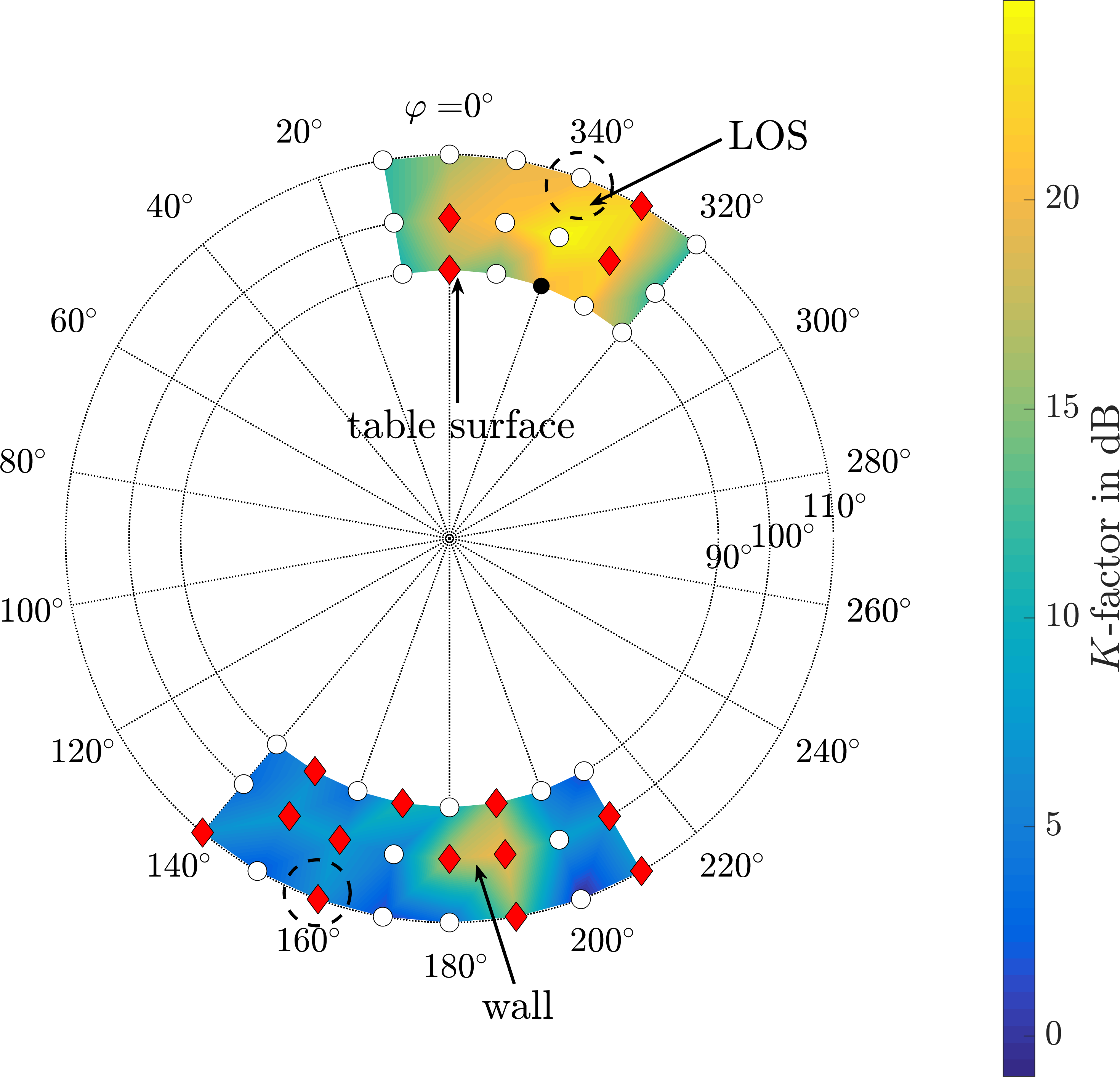
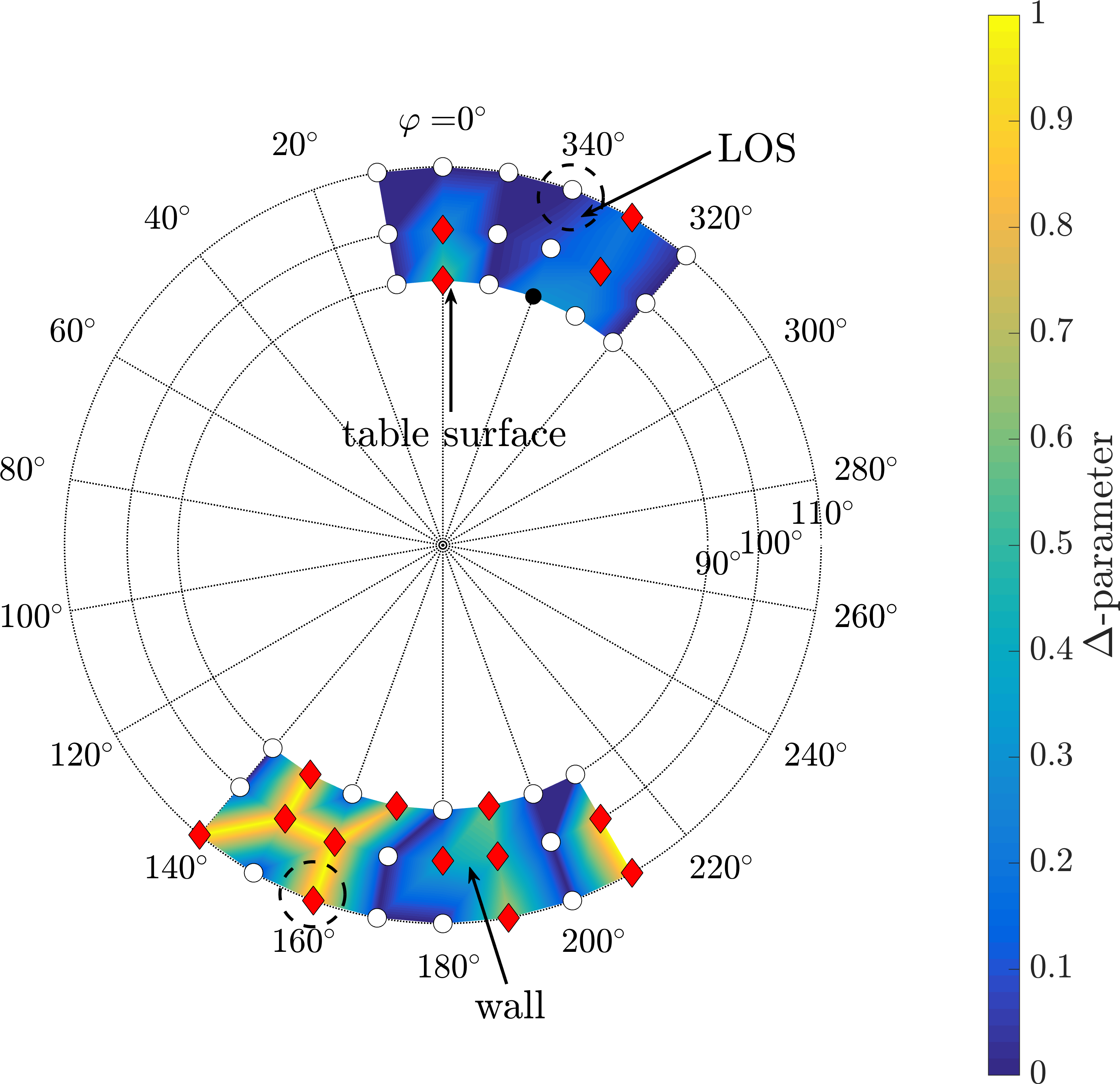
Figure 12: Estimated $K$-factor and $\Delta$-parameter of MC2. Due to the elevated position, the wall reflection has a $6$ dB increased $K$-factor as compared to MC1, see top part of Fig. 7. If the beam is not perfectly aligned, Rician fading turns again into TWDP fading. Wall reflections described by TWDP fading have a $\Delta$-parameter of close to one. The table surface reflection leads to a significantly smaller reflected component ($\Delta\ll 1$). The encircled sampling points are subject of further study in Sections 6 and 7. Markers have the same meaning as in Fig. 6.

6 MC2: Efficient computation of the spatial correlation

The wall reflection from the previous section is now subject to a more detailed study. Our spatial samples are used to show spatial correlations among the drawn samples.

Our three-dimensional sampling problem, see again Fig. 11, is treated via two-dimensional slicing. For the calculation of the spatial (2D) autocorrelation function, we apply the Wiener–Khintchine–Einstein theorem, that relates the autocorrelation function of a wide-sense-stationary random process to its power spectrum [84]. In two dimensions, this theorem reads [85, 86]

$$\mathcal{F}_{2D}\left\{\boldsymbol{C}(x,y)\right\}=S(x^{\prime},y^{\prime})~{},$$ (16)

where $\boldsymbol{C}$ is the 2D-autocorrelation and $S$ is the power spectral density of a 2D signal. The operator $\mathcal{F}_{2D}$ denotes the 2D Fourier transform. We calculate all 2D autocorrelation functions $\boldsymbol{C}^{(z,f)}$ of one $x-y$ slice at height $z$ at a single frequency $f$ through

$$\mathcal{F}_{2D}\big{\{}\boldsymbol{C}^{(z,f)}(x,y)\big{\}}=\mathcal{F}_{2D}\big{\{}\Re\big{\{}\boldsymbol{H}^{(z,f)}\big{(}x^{\prime},y^{\prime}\big{)}\big{\}}\big{\}}$$

$$\hskip 30.1388pt\odot\operatorname{conj}\big{\{}\mathcal{F}_{2D}\big{\{}\Re\big{\{}\boldsymbol{H}^{(z,f)}\big{(}x^{\prime},y^{\prime}\big{)}\big{\}}\big{\}}\big{\}}~{}.$$ (17)

The symbols $\odot$ denotes the Hadamard multiplication. The operator $\operatorname{conj}\{\cdot\}$ denotes complex conjugation. To ensure a real-valued autocorrelation matrix (instead of a generally complex representation [86]), from the complex-valued channel samples only the real parts $\Re\{\cdot\}$ are taken. The spatial autocorrelation of the imaginary parts are identical. One could also analyse the magnitude and phase individually. While the correlation of the magnitude stays almost at 1, the phase correlation patterns are similar to those of the real part.

The 2D Fourier transform $\mathcal{F}_{2D}$ is realised via a 2D discrete Fourier transform (DFT). The 2D DFT is calculated via a multiplication with the DFT matrix $\boldsymbol{D}$ from the left and the right. To mimic a linear convolution with the DFT, zero padding is necessary. We hence take the matrix ${\widetilde{\boldsymbol{H}}}^{(z,f)}$

$$\widetilde{\boldsymbol{H}}^{(z,f)}=\left(\begin{array}[]{cc}\Re\{\boldsymbol{H}^{(z,f)}\}&\boldsymbol{0}\\ \boldsymbol{0}&\boldsymbol{0}\end{array}\right)~{}.$$ (18)

Furthermore, the finite spatial extend of our samples acts as rectangular window. The rectangular window leads to a triangular envelope of the the autocorrelation function. This windowed spatial correlation is denoted by

$$\boldsymbol{C}_{\text{windowed}}^{(z,f)}=\boldsymbol{D}^{H}\bigg{(} \big{(}\boldsymbol{D}{\widetilde{\boldsymbol{H}}}^{(z,f)}\boldsymbol{D}\big{)}$$ (19)

$$\odot\operatorname{conj}\big{\{}\boldsymbol{D}{\widetilde{\boldsymbol{H}}}^{(z,f)}\boldsymbol{D}\big{\}}\bigg{)}\boldsymbol{D}^{H}.$$

To compensate the windowing effect, we calculate the spatial correlation of the rectangular window, constructed in accordance to (18)

$$\boldsymbol{S}=\boldsymbol{D}^{H}\bigg{(} \bigg{(}\boldsymbol{D}\bigg{(}{\begin{array}[]{cc}\mathds{1}&\boldsymbol{0}\\ \boldsymbol{0}&\boldsymbol{0}\end{array}}\bigg{)}\boldsymbol{D}\bigg{)}$$

$$\odot\operatorname{conj}\bigg{\{}\boldsymbol{D}\bigg{(}{\begin{array}[]{cc}\mathds{1}&\boldsymbol{0}\\ \boldsymbol{0}&\boldsymbol{0}\end{array}}\bigg{)}\boldsymbol{D}\bigg{\}}\bigg{)}\boldsymbol{D}^{H}~{}.$$

The matrix $\mathds{1}$ denotes the all-ones matrix. Matrix $\boldsymbol{S}$ compensates the truncation effect of the autocorrelation through element-wise (Hadamard) division, denoted by $\oslash$. Finally, the efficient computation of the spatial correlation (17) reads

$$\boldsymbol{C}^{(z,f)}=\boldsymbol{C}_{\text{windowed}}^{(z,f)}\oslash\boldsymbol{S}~{}.$$ (22)

At a distance of $0.35\lambda$, the measurement data is still correlated, therefore we are able to view our correlation results on the finer, interpolated grid. The interpolation factor is $20$. That means that we calculate our spatial correlations on a grid of $\nicefrac{{0.35\lambda}}{{20}}=0.0175\lambda$ distance. The very efficient implementation of (22) is applied to all (parallel) 2D slices and to all frequencies. All realisations in $z$ and $f$ are averaged

$$\bar{\boldsymbol{C}}=\frac{1}{9}\frac{1}{401}\sum_{z=1}^{9}\sum_{f=1}^{401}\boldsymbol{C}^{(z,f)}~{}.$$ (23)

Furthermore, we plot one-dimensional autocorrelation functions, evaluated along $x$ and $y$, together with their two-dimensional representations. We provide two spatial correlation plots evaluated at an azimuth angle of $\varphi=340^{\circ}$ and $\varphi=160^{\circ}$ in Fig. 13, both at an elevation angle of $\theta=110^{\circ}$. The top part of Fig. 13 shows a correlation pattern dominated by a single wave. The spatial correlation below shows an interference pattern, which is intuitively explained by a superposition of two plane waves. The one dimensional correlations, evaluated either at the $x$-axis or at the $y$-axis, show this oscillatory behaviour as well.

Wall:

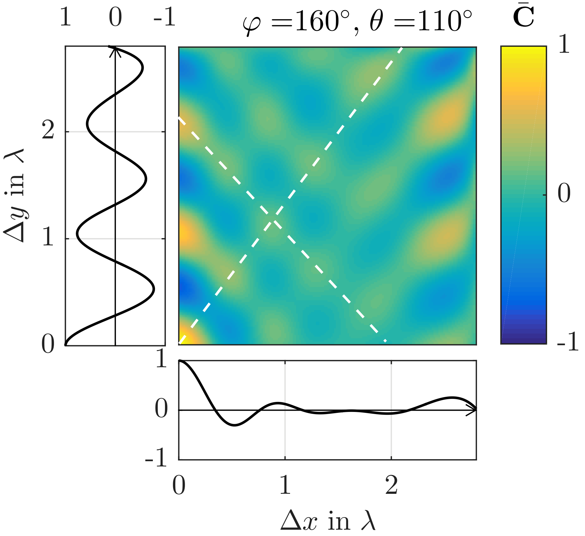
LOS:

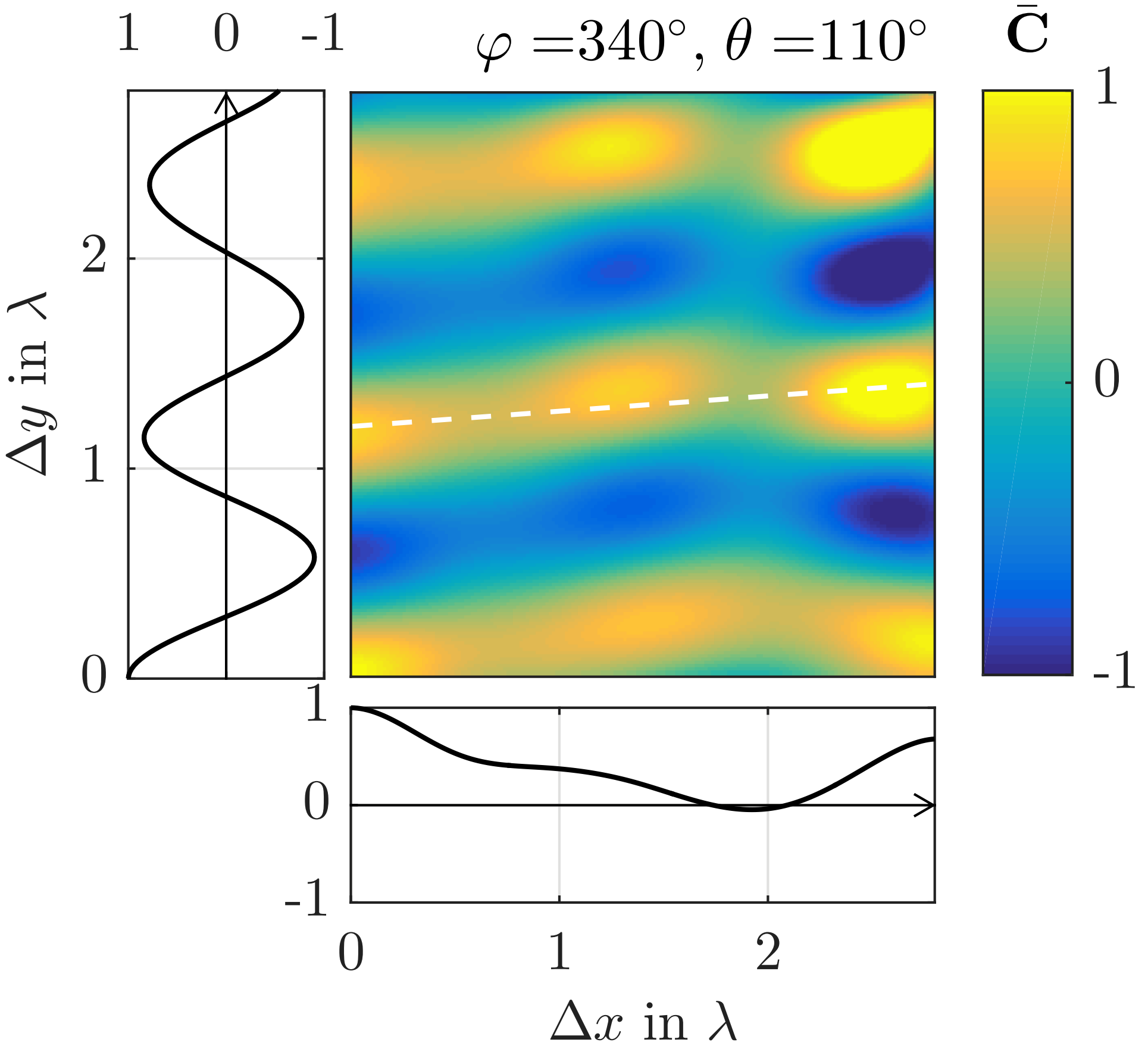
Figure 13: Spatial correlation plot at $\varphi=160^{\circ},340^{\circ}$ and $\theta=110^{\circ}$. For the wall reflection at $\varphi=160^{\circ}$, the pattern shows an interference of two plane waves, supporting the TWDP fading assumption. For LOS at $\varphi=340^{\circ}$, we observe a spatial correlation pattern dominated by one wave. The white dashed lines illustrate plane wave phase fronts.

7 MC2: Time gated fading results

To confirm that our observations are not artefacts of our measurement set-up, for example back-lobes of the horn antenna, we now study the wireless channel in the time domain. Our $2$ GHz wide measurements from MC2 allow for a time resolution of approximately $0.5$ ns. This corresponds to a spatial resolution of $15$ cm. We plot the channel impulse responses as a function of distance, namely the LOS excess length $\Delta s$, that is

$$h(\Delta s)=h\big{(}\big{(}\tau-\tau_{\text{LOS}}\big{)}c_{0}\big{)}~{}.$$ (24)

The scatter-plot of the CIRs for $\varphi=160^{\circ}$ is shown in Fig. 14. The LOS CIR at $\varphi=340^{\circ}$ is displayed as reference as well. The steerable TX is positioned more than a metre apart from the wall. This amounts in an excess distance of approximately two to three metres. At this excess distance, a cluster of multipath components is present. Note, if the horn antenna points towards the wall, the wave emitted by the back-lobe of the horn antenna is received at zero excess distance. Still, the receive power of the back-lobe is far below the components arriving from the wall reflection. Fading is hence determined by the wall scattering behaviour.

Wall:

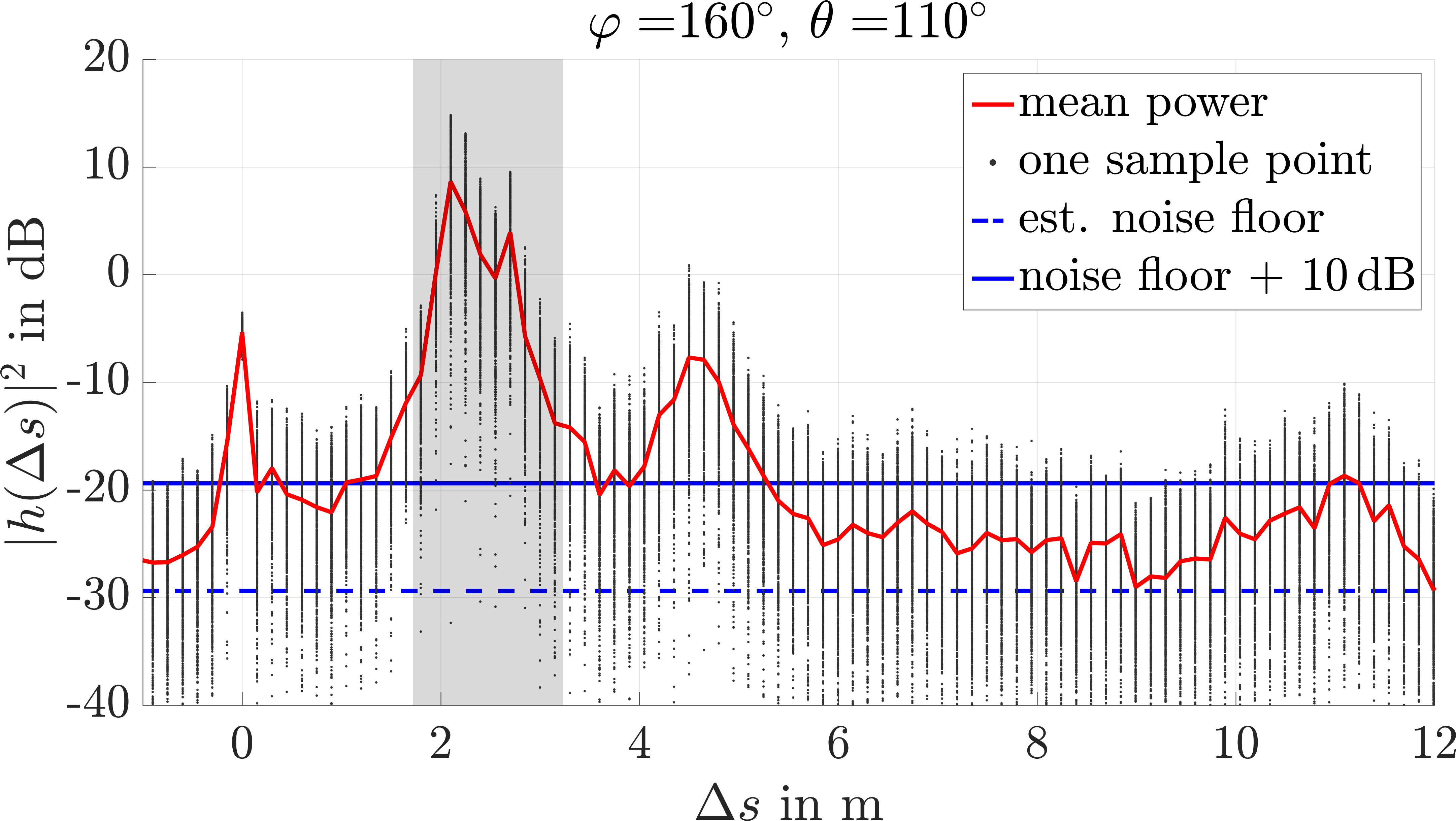
LOS:

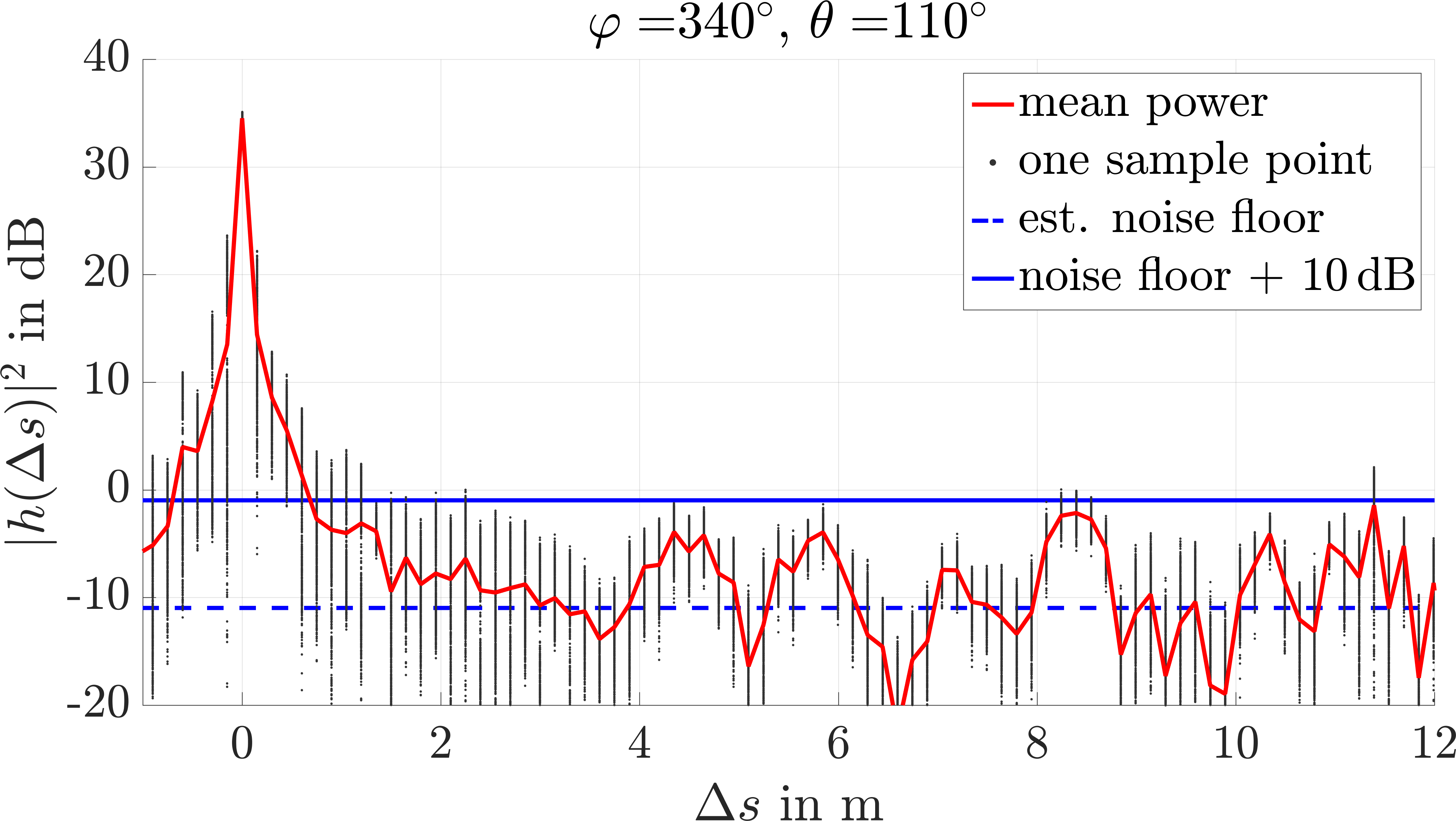
Figure 14: Scatter-plot of the CIRs. We plot the CIRs as a function of spatial distance, where $\Delta s=0$ corresponds to the LOS distance. Our spatial resolution (a channel tap) is $15$ cm. The spatial extend of our sampled cube (729 samples) is $2.8\lambda=1.4$ cm, a magnitude smaller than the spatial resolution. The scatter-plot is evaluated at a wall reflection ($\varphi=160^{\circ}$) and at LOS ($\varphi=340^{\circ}$). The mean power is plotted with a continous red line. We observe that the arrival cluster centred at $2.5$ m fades very deeply. The gray highlighted region around $2.5$ m is further analysed in Fig. 15.

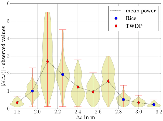
Figure 15: Violin-plot of the CIR time-gated for the wall reflection. This figure shows a zoom-in of the gray highlighted region in Fig. 14. In contrast to Fig. 14, the y-axis is in linear scale. Thereby the violin plot indicates the distribution at each tap. The marker shows the mean value. The marker style codes best fitting distribution.

The gray highlighted region of Fig. 14 (top part) shows a reflection cluster that corresponds to the excess distance of the wall reflection. The distributions of each channel tap are represented by a violin plot in Fig. 15. A violin plot illustrates the distribution estimated via Gaussian kernels [87]. Fig. 15 clearly demonstrates that the TWDP-decided distributions have multiple modes. The AIC decisions are plotted as markers at the mean power levels.

We evaluated the fading statistic in space for $\varphi=160^{\circ}$ at the channel tap corresponding to approximately $2.5$ m excess distance. This channel tap is mid in the cluster belonging to the wall reflection. Fig. 16 clearly shows a TWDP fading behaviour, confirmed by AIC.

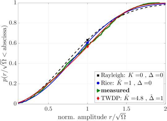
Figure 16: CDF: Distribution fitting for spatial measurement data, time gated by the channel tap at $2.5$ m, $\varphi=160^{\circ}$, and $\theta=110^{\circ}$. Note that, similar to the fitting result in Fig. 2, the estimated Rician K-factor is again much smaller than the TWDP K-factor.

8 Conclusion

We demonstrate, by means of model selection and hypothesis testing, that TWDP fading explains observed indoor millimetre wave channels. Rician fits of reported studies must be considered with caution. As two exemplary fits, in Figs. 2 and 16, show, Rician K-factors tend to be much smaller than their TWDP companions. There is more power in the specular components than is predicted by the Rician fit. The TWDP fading fit accounts for a possible cancellation of two specular waves. Our results are verified through two independent measurement campaigns. For MC1 and MC2 we even used different RF – hardware. While MC1 was limited to results in the frequency-domain, MC2 allowed a careful study in the spatial-domain and the time-domain.

Having this strong evidence at hand, we claim that the TWDP fading model is more accurate to describe mmWave indoor channels. The flexibility of this model allows furthermore to obtain Rician fading ($\Delta=0$) and Rayleigh fading ($K=0$) results with the same channel model.

In link-level simulations, TWDP fading with $\Delta=1$ shows a worse bit error ratio (BER) than Rayleigh fading. To demonstrate this known effect [39, 40, 41, 42, 43], we provide a BER plot in the Appendix. Rayleigh fading can hence not be used as worst case bound, especially for mmWave scenarios.

Appendix - BER and capacity loss for TWDP fading

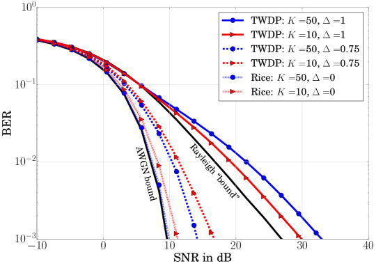
Figure 17: Simulation: Bit error ratio of 4-QAM with TWDP fading. The BER performance of TWDP fading potentially lies above the normally chosen “Rayleigh bound”, for example for $\Delta=1$.

We simulate the BER of 4-QAM transmissions with Gray-mapping and TWDP-fading. The channel is perfectly known to the receiver. The receiver employs a zero-forcing equalizer. The symbols are normalised to symbol power of one, the SNR is the inverse noise power. Our simulations assume frequency flat fading and the only channel tap is generated according to a TWDP statistic. A fading channel tap, given $K$ and $\Delta$, is thus simulated as described by Equation (1). We simulate TWDP flat-fading with independent channel realisations. Rayleigh fading and Rician fading are included as limiting cases and are simulated as references as well, see Fig. 17. As $\Delta$ increases, the BER-performance gets worse and worse, confer the dashed line for $\Delta=0.5$. Finally, Fig. 17 shows the worse-than-Rayleigh regions [42] for $\Delta=1$.

At this point, we would like to point out that the uncoded BER, of course, has little significance. The maximum capacity loss $\delta_{C}$ (in bit/s/Hz) occurs as $K\rightarrow\infty$ and is bounded by [35]

$$\delta_{C}(K\rightarrow\infty,\Delta)=1-\log_{2}(1+\sqrt{1-\Delta^{2}})\leq 1~{}.$$ (25)

DFT

discrete Fourier transform

mmWave

millimetre wave

AWG

arbitrary waveform generator

PLL

phase-locked loop

SNR

signal-to-noise ratio

SA

signal analyser

LO

local oscillator

RF

radio frequency

RX

receiver

TX

transmitter

CDF

cumulative distribution function

AIC

Akaike’s information criterion

TWDP

two-wave with diffuse power

LOS

line-of-sight

NLOS

non-line-of-sight

IQ

in-phase and quadrature

CDF

cumulative distribution function

PDF

probability density function

BER

bit error ratio

MC1

first measurement campaign

MC2

second measurement campaign

VNA

vector network analyser

CIR

channel impulse response

MPC

multipath component

References

- [1] Martin Steinbauer, Andreas F Molisch, and Ernst Bonek. The double-directional radio channel. IEEE Antennas and Propagation Magazine, 43(4):51–63, 2001.
- [2] Christopher R Anderson and Theodore S Rappaport. In-building wideband partition loss measurements at 2.5 and 60 GHz. IEEE Transactions on Wireless Communications, 3(3):922–928, 2004.
- [3] Nektarios Moraitis and Philip Constantinou. Measurements and characterization of wideband indoor radio channel at 60 GHz. IEEE Transactions on Wireless Communications, 5(4):880–889, 2006.
- [4] Suiyan Geng, Jarmo Kivinen, Xiongwen Zhao, and Pertti Vainikainen. Millimeter-wave propagation channel characterization for short-range wireless communications. IEEE Transactions on Vehicular Technology, 58(1):3–13, 2009.
- [5] Karma Wangchuk, Kento Umeki, Tatsuki Iwata, Panawit Hanpinitsak, Minseok Kim, Kentaro Saito, and Jun-ichi Takada. Double directional millimeter wave propagation channel measurement and polarimetric cluster properties in outdoor urban pico-cell environment. IEICE Transactions on Communications, 100(7):1133–1144, 2017.
- [6] Michael Peter, Wilhelm Keusgen, and Richard J Weiler. On path loss measurement and modeling for millimeter-wave 5G. In Proc. of 9th European Conference on Antennas and Propagation (EuCAP), pages 1–5. IEEE, 2015.
- [7] Michael Peter, Richard J Weiler, Barış Göktepe, Wilhelm Keusgen, and Kei Sakaguchi. Channel measurement and modeling for 5G urban microcellular scenarios. Sensors, 16(8):1330, 2016.
- [8] Mathew K Samimi, Theodore S Rappaport, and George R MacCartney. Probabilistic omnidirectional path loss models for millimeter-wave outdoor communications. IEEE Wireless Communications Letters, 4(4):357–360, 2015.
- [9] Sijia Deng, Mathew K Samimi, and Theodore S Rappaport. 28 GHz and 73 GHz millimeter-wave indoor propagation measurements and path loss models. In Proc. of IEEE International Conference on Communication Workshop (ICCW), pages 1244–1250. IEEE, 2015.
- [10] George R MacCartney, Theodore S Rappaport, Mathew K Samimi, and Shu Sun. Millimeter-wave omnidirectional path loss data for small cell 5G channel modeling. IEEE Access, 3:1573–1580, 2015.
- [11] Wonil Roh, Ji-Yun Seol, Jeongho Park, Byunghwan Lee, Jaekon Lee, Yungsoo Kim, Jaeweon Cho, Kyungwhoon Cheun, and Farshid Aryanfar. Millimeter-wave beamforming as an enabling technology for 5G cellular communications: Theoretical feasibility and prototype results. IEEE Communications Magazine, 52(2):106–113, 2014.
- [12] Sooyoung Hur, Taejoon Kim, David J Love, James V Krogmeier, Timothy A Thomas, and Amitava Ghosh. Millimeter wave beamforming for wireless backhaul and access in small cell networks. IEEE Transactions on Communications, 61(10):4391–4403, 2013.
- [13] Shu Sun, Theodore S Rappaport, Robert W Heath, Andrew Nix, and Sundeep Rangan. MIMO for millimeter-wave wireless communications: Beamforming, spatial multiplexing, or both? IEEE Communications Magazine, 52(12):110–121, 2014.
- [14] Zhouyue Pi and Farooq Khan. An introduction to millimeter-wave mobile broadband systems. IEEE Communications Magazine, 49(6), 2011.
- [15] Robert W Heath, Nuria Gonzalez-Prelcic, Sundeep Rangan, Wonil Roh, and Akbar M Sayeed. An overview of signal processing techniques for millimeter wave MIMO systems. IEEE Journal of Selected Topics in Signal Processing, 10(3):436–453, 2016.
- [16] Jeffrey G Andrews, Tianyang Bai, Mandar N Kulkarni, Ahmed Alkhateeb, Abhishek K Gupta, and Robert W Heath. Modeling and analyzing millimeter wave cellular systems. IEEE Transactions on Communications, 65(1):403–430, 2017.
- [17] Ahmed Alkhateeb, Omar El Ayach, Geert Leus, and Robert W Heath. Channel estimation and hybrid precoding for millimeter wave cellular systems. IEEE Journal of Selected Topics in Signal Processing, 8(5):831–846, 2014.
- [18] Mandar N Kulkarni, Amitava Ghosh, and Jeffrey G Andrews. A comparison of MIMO techniques in downlink millimeter wave cellular networks with hybrid beamforming. IEEE Transactions on Communications, 64(5):1952–1967, 2016.
- [19] Erich Zöchmann, Stefan Schwarz, and Markus Rupp. Comparing antenna selection and hybrid precoding for millimeter wave wireless communications. In Proc. of IEEE Sensor Array and Multichannel Signal Processing Workshop (SAM), pages 1–5. IEEE, 2016.
- [20] Stefan Pratschner, Sebastian Caban, Stefan Schwarz, and Markus Rupp. A mutual coupling model for massive MIMO applied to the 3GPP 3D channel model. In Proc. of 25th European Signal Processing Conference (EUSIPCO), pages 623–627. IEEE, 2017.
- [21] John Brady, Nader Behdad, and Akbar M Sayeed. Beamspace MIMO for millimeter-wave communications: System architecture, modeling, analysis, and measurements. IEEE Transactions on Antennas and Propagation, 61(7):3814–3827, 2013.
- [22] Yong Zeng and Rui Zhang. Millimeter wave MIMO with lens antenna array: A new path division multiplexing paradigm. IEEE Transactions on Communications, 64(4):1557–1571, 2016.
- [23] Yong Zeng and Rui Zhang. Cost-effective millimeter-wave communications with lens antenna array. IEEE Wireless Communications, 24(4):81–87, 2017.
- [24] Gregory D Durgin. Space-time wireless channels. Prentice Hall Professional, Upper Saddle River, 2003.
- [25] Diego Dupleich, Naveed Iqbal, Christian Schneider, Stephan Haefner, Robert Müller, Sergii Skoblikov, Jian Luo, and Reiner Thomä. Investigations on fading scaling with bandwidth and directivity at 60 GHz. In Proc. of 11th European Conference on Antennas and Propagation (EUCAP), pages 3375–3379. IEEE, 2017.
- [26] Naveed Iqbal, Christian Schneider, Jian Luo, Diego Dupleich, Robert Müller, Stephan Haefner, and Reiner S Thomä. On the stochastic and deterministic behavior of mmWave channels. In Proc. of 11th European Conference on Antennas and Propagation (EUCAP), pages 1813–1817. IEEE, 2017.
- [27] Mathew K Samimi, George R MacCartney, Shu Sun, and Theodore S Rappaport. 28 GHz millimeter-wave ultrawideband small-scale fading models in wireless channels. In Proc. of Vehicular Technology Conference (VTC Spring), pages 1–6. IEEE, 2016.
- [28] Shu Sun, Hangsong Yan, George R MacCartney, and Theodore S Rappaport. Millimeter wave small-scale spatial statistics in an urban microcell scenario. In Proc. of IEEE International Conference on Communications (ICC), pages 1–7. IEEE, 2017.
- [29] Theodore S Rappaport, George R MacCartney, Shu Sun, Hangsong Yan, and Sijia Deng. Small-scale, local area, and transitional millimeter wave propagation for 5G communications. IEEE Transactions on Antennas and Propagation, 2017.
- [30] Theodoros Mavridis, Luca Petrillo, Julien Sarrazin, Aziz Benlarbi-Delai, and Philippe De Doncker. Near-body shadowing analysis at 60 GHz. IEEE Transactions on Antennas and Propagation, 63(10):4505–4511, 2015.
- [31] Gregory D Durgin, Theodore S Rappaport, and David A De Wolf. New analytical models and probability density functions for fading in wireless communications. IEEE Transactions on Communications, 50(6):1005–1015, 2002.
- [32] Raffaele Esposito and L Wilson. Statistical properties of two sine waves in Gaussian noise. IEEE Transactions on Information Theory, 19(2):176–183, 1973.
- [33] Soon H Oh and Kwok H Li. BER performance of BPSK receivers over two-wave with diffuse power fading channels. IEEE Transactions on Wireless Communications, 4(4):1448–1454, 2005.
- [34] Seyed Ali Saberali and Norman C Beaulieu. New expressions for TWDP fading statistics. IEEE Wireless Communications Letters, 2(6):643–646, 2013.
- [35] Milind Rao, F Javier Lopez-Martinez, Mohamed-Slim Alouini, and Andrea Goldsmith. MGF approach to the analysis of generalized two-ray fading models. IEEE Transactions on Wireless Communications, 14(5):2548–2561, 2015.
- [36] Juan M Romero-Jerez, F Javier Lopez-Martinez, José F Paris, and Andrea J Goldsmith. The fluctuating two-ray fading model: Statistical characterization and performance analysis. IEEE Transactions on Wireless Communications, 2017.
- [37] Stefan Schwarz. Outage investigation of beamforming over random-phase finite-scatterer MISO channels. IEEE Signal Processing Letters, 2017.
- [38] S. Schwarz. Outage-based multi-user admission control for random-phase finite-scatterer MISO channels. In Proc. of IEEE Vehicular Technology Conference (VTC-Fall), pages 1–5, Toronto, Canada, Sept. 2017.
- [39] Jeff Frolik. A case for considering hyper-Rayleigh fading channels. IEEE Transactions on Wireless Communications, 6(4), 2007.
- [40] Jeff Frolik. On appropriate models for characterizing hyper-Rayleigh fading. IEEE Transactions on Wireless Communications, 7(12), 2008.
- [41] Jeff Frolik, Thomas M Weller, Stephen DiStasi, and James Cooper. A compact reverberation chamber for hyper-Rayleigh channel emulation. IEEE Transactions on Antennas and Propagation, 57(12):3962–3968, 2009.
- [42] David W Matolak and Jeff Frolik. Worse-than-Rayleigh fading: Experimental results and theoretical models. IEEE Communications Magazine, 49(4), 2011.
- [43] Lu’ay Bakir and Jeff Frolik. Diversity gains in two-ray fading channels. IEEE Transactions on Wireless Communications, 8(2):968–977, 2009.
- [44] Erich Zöchmann, Ke Guan, and Markus Rupp. Two-ray models in mmWave communications. In Proc. of Workshop on Signal Processing Advances in Wireless Communications (SPAWC), pages 1–5, 2017.
- [45] Erich Zöchmann, Martin Lerch, Sebastian Caban, Robert Langwieser, Christoph Mecklenbräuker, and Markus Rupp. Directional evaluation of receive power, Rician K-factor and RMS delay spread obtained from power measurements of 60 GHz indoor channels. In Proc. of IEEE Topical Conference on Antennas and Propagation in Wireless Communications (APWC), pages 1–4, 2016.
- [46] Erich Zöchmann, Martin Lerch, Stefan Pratschner, Ronald Nissel, Sebastian Caban, and Markus Rupp. Associating spatial information to directional millimeter wave channel measurements. In Proc. of IEEE Vehicular Technology Conference (VTC-Fall), pages 1–5, 2017.
- [47] Kenneth P Burnham and David R Anderson. Model selection and multimodel inference: a practical information-theoretic approach. Springer Science & Business Media, New York, 2003.
- [48] Robert W Frick. The appropriate use of null hypothesis testing. Psychological Methods, 1(4):379, 1996.
- [49] Constantine A Balanis. Antenna theory: analysis and design. John Wiley & Sons, Hoboken, 2005.
- [50] James O Berger and William H Jefferys. The application of robust Bayesian analysis to hypothesis testing and Occam’s razor. Journal of the Italian Statistical Society, 1(1):17–32, 1992.
- [51] Alberto Maydeu-Olivares and C Garcia-Forero. Goodness-of-fit testing. International encyclopedia of education, 7(1):190–196, 2010.
- [52] Ulrich G Schuster and Helmut Bolcskei. Ultrawideband channel modeling on the basis of information-theoretic criteria. IEEE Transactions on Wireless Communications, 6(7), 2007.
- [53] Hirotugu Akaike. A new look at the statistical model identification. IEEE Transactions on Automatic Control, 19(6):716–723, 1974.
- [54] Thomas M Ludden, Stuart L Beal, and Lewis B Sheiner. Comparison of the Akaike information criterion, the Schwarz criterion and the F test as guides to model selection. Journal of Pharmacokinetics and Biopharmaceutics, 22(5):431–445, 1994.
- [55] Kenneth P Burnham and David R Anderson. Multimodel inference: understanding AIC and BIC in model selection. Sociological Methods & Research, 33(2):261–304, 2004.
- [56] Ruisi He, Andreas F Molisch, Fredrik Tufvesson, Zhangdui Zhong, Bo Ai, and Tingting Zhang. Vehicle-to-vehicle propagation models with large vehicle obstructions. IEEE Transactions on Intelligent Transportation Systems, 15(5):2237–2248, 2014.
- [57] Telmo Santos, Fredrik Tufvesson, and Andreas F Molisch. Modeling the ultra-wideband outdoor channel: Model specification and validation. IEEE Transactions on Wireless Communications, 9(6), 2010.
- [58] Ruisi He, Zhangdui Zhong, Bo Ai, Gongpu Wang, Jianwen Ding, and Andreas F Molisch. Measurements and analysis of propagation channels in high-speed railway viaducts. IEEE Transactions on Wireless Communications, 12(2):794–805, 2013.
- [59] Ke Guan, Zhangdui Zhong, Bo Ai, and Thomas Kürner. Propagation measurements and modeling of crossing bridges on high-speed railway at 930 MHz. IEEE Transactions on Vehicular Technology, 63(2):502–517, 2014.
- [60] Ruisi He, Zhangdui Zhong, Bo Ai, Jianwen Ding, Yaoqing Yang, and Andreas F Molisch. Short-term fading behavior in high-speed railway cutting scenario: Measurements, analysis, and statistical models. IEEE Transactions on Antennas and Propagation, 61(4):2209–2222, 2013.
- [61] Donggu Kim, Hoojin Lee, and Joonhyuk Kang. Comments on “Near-body shadowing analysis at 60 GHz”. IEEE Transactions on Antennas and Propagation, 65(6):3314–3314, 2017.
- [62] Jesús Lopez-Fernandez, Laureano Moreno-Pozas, Francisco Javier Lopez-Martinez, and Eduardo Martos-Naya. Joint parameter estimation for the two-wave with diffuse power fading model. Sensors, 16(7):1014, 2016.
- [63] Jesús Lopez-Fernandez, Laureano Moreno-Pozas, Eduardo Martos-Naya, and F Javier López-Martínez. Moment-based parameter estimation for the two-wave with diffuse power fading model. In Proc. of the 84th IEEE Vehicular Technology Conference (VTC-Fall), pages 1–5. IEEE, 2016.
- [64] Arthur Stanley Goldberger. Econometric Theory. John Wiley & Sons, New York, 1964.
- [65] John H McDonald. Handbook of biological statistics, volume 2. Sparky House Publishing Baltimore, MD, Baltimore, 2009.
- [66] Barnet Woolf. The log likelihood ratio test (the g-test): Methods and tables for tests of heterogeneity in contingency tables. Annals of Human Genetics, 21(4):397–409, 1957.
- [67] Jesse Hoey. The two-way likelihood ratio (G) test and comparison to two-way Chi squared test. arXiv preprint arXiv:1206.4881, 2012.
- [68] Quentin H Spencer, Brian D Jeffs, Michael A Jensen, and A Lee Swindlehurst. Modeling the statistical time and angle of arrival characteristics of an indoor multipath channel. IEEE Journal on Selected Areas in Communications, 18(3):347–360, 2000.
- [69] Gregory D Durgin, Vikas Kukshya, and Theodore S Rappaport. Wideband measurements of angle and delay dispersion for outdoor and indoor peer-to-peer radio channels at 1920 MHz. IEEE Transactions on Antennas and Propagation, 51(5):936–944, 2003.
- [70] F. Fuschini, S. Häfner, M. Zoli, R. Müller, E. M. Vitucci, D. Dupleich, M. Barbiroli, J. Luo, E. Schulz, V. Degli-Esposti, and R. S. Thomä. Analysis of in-room mm-Wave propagation: Directional channel measurements and ray tracing simulations. Journal of Infrared, Millimeter, and Terahertz Waves, 38(6):727–744, 2017.
- [71] Joni Vehmas, Jan Jarvelainen, Sinh Le Hong Nguyen, Reza Naderpour, and Katsuyuki Haneda. Millimeter-wave channel characterization at Helsinki airport in the 15, 28, and 60 GHz bands. In Proc. of IEEE Vehicular Technology Conference (VTC-Fall), 2016.
- [72] Andreas F Molisch. Wireless communications, volume 34. John Wiley & Sons, Chichester, 2012.
- [73] Pasternack 60 GHz transmitter and 60 GHz receiver modules.
- [74] Per Zetterberg and Ramin Fardi. Open source SDR frontend and measurements for 60-GHz wireless experimentation. IEEE Access, 3:445–456, 2015.
- [75] Seun Sangodoyin, Jussi Salmi, S Niranjayan, and Andreas F Molisch. Real-time ultrawideband MIMO channel sounding. In Proc. of Antennas and Propagation Conference (EUCAP). IEEE, 2012.
- [76] Minseok Kim, Hung Kinh Pham, Yuyuan Chang, and Jun-ichi Takada. Development of low-cost 60-GHz millimeter-wave channel sounding system. In Proc. of Global Symposium on Millimeter Wave (GSMM), 2013.
- [77] Erich Zöchmann, Christoph Mecklenbräuker, Martin Lerch, Stefan Pratschner, Markus Hofer, David Löschenbrand, Jiri Blumenstein, Seun Sangodoyin, Gerald Artner, Sebastian Caban, Thomas Zemen, Ales Prokes, Markus Rupp, and Andreas F. Molisch. Measured delay and Doppler profiles of overtaking vehicles at 60 GHz. In Proc. of the 12th European Conference on Antennas and Propagation (EuCAP), pages 1–5. IEEE, 2018.
- [78] Martin Lerch, Erich Zöchmann, Sebastian Caban, and Markus Rupp. Noise bounds in multicarrier mmWave Doppler measurements. In Proc. of European Wireless, 2017.
- [79] Ronald Nissel, Erich Zöchmann, Martin Lerch, Sebastian Caban, and Markus Rupp. Low latency MISO FBMC-OQAM: It works for millimeter waves! In Proc. of IEEE International Microwave Symposium (IMS), 2017.
- [80] Martin Lerch, Sebastian Caban, Martin Mayer, and Markus Rupp. The Vienna MIMO testbed: Evaluation of future mobile communications techniques. Intel Technology Journal, 18(3), 2014.
- [81] Sebastian Caban, Armin Disslbacher-Fink, José A García-Naya, and Markus Rupp. Synchronization of wireless radio testbed measurements. In Proc. of IEEE Instrumentation and Measurement Technology Conference (I2MTC), pages 1–4. IEEE, 2011.
- [82] Markus Laner, Sebastian Caban, Philipp Svoboda, and Markus Rupp. Time synchronization performance of desktop computers. In Proc. of IEEE Symposium on Precision Clock Synchronization for Measurement Control and Communication (ISPCS), pages 75–80. IEEE, 2011.
- [83] Robert Haining. Spatial data analysis in the social and environmental sciences. Cambridge University Press, Cambridge, 1993.
- [84] Alexander Khintchine. Korrelationstheorie der stationären stochastischen Prozesse. Mathematische Annalen, 109(1):604–615, 1934.
- [85] Todd A Ell and Stephen J Sangwine. Hypercomplex Wiener-Khintchine theorem with application to color image correlation. In Proc. of International Conference on Image Processing, volume 2, pages 792–795. IEEE, 2000.
- [86] C Eddie Moxey, Stephen J Sangwine, and Todd A Ell. Hypercomplex correlation techniques for vector images. IEEE Transactions on Signal Processing, 51(7):1941–1953, 2003.
- [87] Jerry L Hintze and Ray D Nelson. Violin plots: a box plot-density trace synergism. The American Statistician, 52(2):181–184, 1998.