Quantum Trajectory Distribution for Weak Measurement
of a Superconducting Qubit: Experiment meets Theory

Abstract

Quantum measurements are described as instantaneous projections in textbooks. They can be stretched out in time using weak measurements, whereby one can observe the evolution of a quantum state as it heads towards one of the eigenstates of the measured operator. This evolution can be understood as a continuous nonlinear stochastic process, generating an ensemble of quantum trajectories, consisting of noisy fluctuations on top of geodesics that attract the quantum state towards the measured operator eigenstates. The rate of evolution is specific to each system-apparatus pair, and the Born rule constraint requires the magnitudes of the noise and the attraction to be precisely related. We experimentally observe the entire quantum trajectory distribution for weak measurements of a superconducting qubit in circuit QED architecture, quantify it, and demonstrate that it agrees very well with the predictions of a single-parameter white-noise stochastic process. This characterisation of quantum trajectories is a powerful clue to unraveling the dynamics of quantum measurement, beyond the conventional axiomatic quantum theory.

Motivation: The textbook formulation of quantum mechanics describes measurement according to the von Neumann projection postulate, which states that one of the eigenvalues of the measured observable is the measurement outcome and the post-measurement state is the corresponding eigenvector. With $P_{i}$ denoting the projection operator for the eigenstate $|i\rangle$,

$$|\psi\rangle\longrightarrow P_{i}|\psi\rangle/|P_{i}|\psi\rangle|,$$ (1)

$$P_{i}=P_{i}^{\dagger},~{}~{}P_{i}P_{j}=P_{i}\delta_{ij},~{}~{} \sum_{i}P_{i}=I.$$ (2)

This change is sudden, irreversible, consistent on repetition, and probabilistic in the choice of “$i$”. Which “$i$” would occur in a particular experimental run, is not specified; only the probabilities of various outcomes are specified, requiring an ensemble interpretation for the outcomes. These probabilities follow the Born rule,

$$prob(i)=\langle\psi|P_{i}|\psi\rangle=Tr(P_{i}\rho)~{},~{}~{}\rho\longrightarrow\sum_{i}P_{i}\rho P_{i}~{},$$ (3)

and the ensemble evolution takes initially pure states to mixed states.

Over the years, many attempts have been made to unravel the dynamics of this process Wheeler ; Braginsky . The framework of environmental decoherence is an important step that provides continuous interpolation of the sudden projection. In this framework, both the system and its environment (which includes the measuring apparatus) follow the unitary Schrödinger evolution, and the unobserved degrees of freedom of the environment are “summed over” to determine how the remaining observed degrees of freedom evolve. The result is still an ensemble description, but it provides a quantitative understanding of how the off-diagonal elements of the reduced density matrix $\rho$ decay Zeh ; Wiseman . Subsequently, solution of the “measurement problem” requires decomposing the ensemble into individual quantum contributions (i.e. which “$i$” will occur in which experimental run), and that forces us to look beyond the closed unitary Schrödinger evolution.

Some of the attempted decompositions of the quantum ensemble are physical, e.g. introduction of hidden variables with novel dynamics or ignored interactions with known dynamics Bohm ; Ghirardirev ; Penrose ; Bassirev . Some other attempts philosophically question what is real and what is observable, in principle as well as by human beings with limited capacity Everett ; GMH ; QBism . Although these attempts are not theoretically inconsistent, none of them have been positively verified by experiments—either they are untestable or only bounds exist on their parameters Bassirev ; Bassi .

We focus here on the extension of quantum mechanics that describes the measurement as a continuous nonlinear stochastic process. It is a particular case of the class of stochastic collapse models that add a measurement driving term and a random noise term to the Schrödinger evolution Bassirev . We look at these terms in an effective theory approach, without assuming a specific collapse basis (e.g. energy or position basis) or a specific collapse interaction (e.g. gravity or some other universal interaction). In this expanded view, the collapse process can be specific to each system-apparatus pair and need not be universal. Such a setting is necessary to understand the quantum state evolution during continuous measurements of superconducting transmon qubits VijayRev , where the collapse basis as well as the system-apparatus interaction strength can be varied by changing the control parameters and without changing the apparatus mass or size or position.

Realisation of quantum measurement as a continuous stochastic process is tightly constrained by the well-established properties of quantum dynamics Pearle ; Gisin ; Diosi . A precise combination of the attraction towards the eigenstates and unbiased noise is needed to reproduce the Born rule as a constant of evolution Gisin . Two of us have emphasised recently that this is a fluctuation-dissipation relation BornRule . It points to a common origin for the stochastic and the deterministic contributions to the measurement evolution, analogous to both diffusion and viscous damping arising from the same underlying molecular scattering in statistical physics. Moreover, for a binary measurement (i.e. when the measured operator has only two eigenvalues), the complete quantum trajectory distribution is predicted in terms of only a single dimensionless evolution parameter.

In this work, we experimentally observe quantum trajectories for superconducting qubits, using weak measurements Bub that stretch out the evolution time from the initial state to the final projected state. Going beyond previous experiments Murch ; Weber that deduced the most likely evolution paths from the observed trajectories, we quantitatively compare the entire observed trajectory distribution with the single parameter theoretical prediction, to test the validity of the nonlinear stochastic evolution model. We also observe the quantum trajectories for time scales going up to the relaxation time; the relaxation substantially alters the evolution, and we show that the relaxation effects can be successfully described by a simple modification of the theoretical model.

Theoretical Predictions: We consider evolution of a qubit undergoing binary weak measurement in absence of any driving Hamiltonian, and explicitly include the effect of a finite excited state relaxation time $T_{1}$. In the continuous stochastic quantum measurement model, the evolution depends on the nature of the noise; we consider the particular case of white noise that is appropriate for weak measurements of transmons Korotkov . In this quantum diffusion scenario, with $|0\rangle$ and $|1\rangle$ as the measurement eigenstates, the density matrix evolves according to qubitevol :

$${d\over dt}\rho_{00}=2g(w_{0}-w_{1})~{}\rho_{00}~{}\rho_{11}+{1\over T_{1}}\rho_{11}~{}.$$ (4)

Here $g(t)$ is the system-apparatus coupling, and $w_{i}(t)$ are real weights representing evolution towards the two eigenstates. The weights satisfy $w_{0}+w_{1}=1$, and

$$w_{0}-w_{1}=\rho_{00}-\rho_{11}+\sqrt{S_{\xi}}~{}\xi~{},$$ (5)

where the unbiased white noise with spectral density $S_{\xi}$ obeys $\langle\!\langle\xi(t)\rangle\!\rangle=0$ and $\langle\!\langle\xi(t)\xi(t^{\prime})\rangle\!\rangle=\delta(t-t^{\prime})$.

This evolution is a stochastic differential process on the interval $[0,1]$, with perfectly absorbing boundaries. The Born rule becomes a constant of evolution when $gS_{\xi}=1$ Pearle ; Gisin , which we impose henceforth. The Itô form is convenient for numerical simulations of quantum trajectories:

$$d\rho_{00}=2\sqrt{g}~{}\rho_{00}~{}\rho_{11}~{}dW+(1/T_{1})\rho_{11}~{}dt~{},$$ (6)

where the Wiener increment satisfies $\langle\!\langle dW(t)\rangle\!\rangle=0$ and $(dW(t))^{2}=dt$. Although we are unable to integrate Eq.(6) exactly, exact integrals of each of the two terms on its right-hand-side are known. We simulate quantum trajectories using a Gaussian distribution for $dW$ and a symmetric Trotter-type integration scheme. The discretisation error is then $O((dt)^{2})$ for individual steps, and is made negligible by making $dt$ sufficiently small.

The probability distribution of the quantum trajectories, $p(\rho_{00},t)$, obeys the Fokker-Planck equation:

$${\partial p(\rho_{00},t)\over\partial t} = 2g{\partial^{2}\over\partial^{2}\rho_{00}}\Big{(}\rho_{00}^{2}\rho_{11}^{2}p(\rho_{00},t)\Big{)}$$ (7)

$$- {1\over T_{1}}{\partial\over\partial\rho_{00}}\Big{(}\rho_{11}p(\rho_{00},t)\Big{)}~{}.$$

Its solution is easier to visualise after the map

$$\tanh(z)=2\rho_{00}-1=\rho_{00}-\rho_{11}~{},$$ (8)

from $\rho_{00}\in[0,1]$ to $z\in[-\infty,\infty]$. With the initial condition $p(\rho_{00},0)=\delta(x)$, and in absence of any relaxation, the exact solution consists of two non-interfering parts with areas $x$ and $1-x$, monotonically travelling to the boundaries at $\rho_{00}=1$ and $0$ respectively Pearle ; Gisin ; pathintdist . In terms of the variable $z$, these parts of $p(z,t)$ are Gaussians, with centres at $z_{\pm}(t)=\tanh^{-1}(2x-1)\pm gt$ and common variance $gt$. Excited state relaxation introduces an additional drift in the evolution, which makes the part heading to $\rho_{00}=1$ grow at the expense of the part heading to $\rho_{00}=0$.

Other than the unavoidable relaxation time $T_{1}$, the entire quantum trajectory distribution is determined in terms of the single dimensionless evolution parameter $\tau(g,t)\equiv\int_{0}^{t}g(t^{\prime})dt^{\prime}$. A strong measurement, $\tau>10$ strongtau , is essentially a projective measurement. In weak measurement experiments on transmons, the coupling $g$ is a tunable parameter, and the intervening stages between the initial state and the final projective outcome can be observed as $\tau$ gradually increases. We next present the results of such an experiment.

Experimental Results: Our experiments were carried out on superconducting 3D transmon qubits, placed inside a microwave resonator cavity and dispersively coupled to it. The transmon is a nonlinear oscillator transmonref , consisting of a Josephson junction shunted by a capacitor; the two lowest quantum levels are treated as a qubit, which possesses good coherence and is insensitive to charge noise. Measurements of the qubit are performed in the circuit QED architecture VijayRev , by probing the cavity with a resonant microwave pulse; the amplitude of the microwave pulse controls the measurement strength. The scattered wave is amplified by a near-quantum-limited Josephson parametric amplifier JPA operated in the phase-sensitive mode, so that only the quadrature containing information about the $\sigma_{z}$ component of the qubit is amplified VijayRev . The amplified single-quadrature signal is extracted as a measurement current using standard homodyne detection. We provide more details of the device and the experimental setup in the Supplementary Information.

The qubit eigenstates produce Gaussian distributions for the measurement current, centred at $I_{0}$ and $I_{1}$, and with variance $\sigma^{2}$ spline . The measurements are weak when $\Delta I=|I_{0}-I_{1}|\ll\sigma$, as illustrated in Fig. 1. The integrated current measurement gives the quantum trajectory evolution, according to the Bayesian prescription Korotkov (note that $\rho_{11}=1-\rho_{00}$):

$${\rho_{00}(t+\Delta t)\over\rho_{11}(t+\Delta t)} = {\rho_{00}(t)\over\rho_{11}(t)}{\exp[-(I_{m}(\Delta t)-I_{0})^{2}/2\sigma^{2}]\over\exp[-(I_{m}(\Delta t)-I_{1})^{2}/2\sigma^{2}]}~{},$$ (9)

$$I_{m}(\Delta t) = {1\over\Delta t}\int_{0}^{\Delta t}I(t^{\prime})~{}dt^{\prime}~{}.$$ (10)

Simultaneous relaxation of the excited state produces:

$$\rho_{11}(t+\Delta t)=\rho_{11}(t)\exp(-\Delta t/T_{1})~{}.$$ (11)

We construct complete quantum trajectories by combining these two evolutions in a symmetric Trotter-type scheme. This construction has been shown to be fully consistent with direct quantum state tomography at any time $t$ Murch ; even though the measurement extracts only partial information, its back-action on the qubit is completely known, and the qubit evolution from a known starting state can be precisely constructed Hatridge ; Murch .

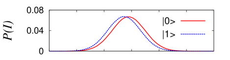
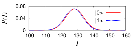
Figure 1: Measurement current distributions for the qubit eigenstates after evolution for $0.5\mu s$, for an ensemble of $10^{6}$ trajectories. They are Gaussians to high accuracy. The bottom figure corresponds to a weaker system-apparatus coupling than the top one. The system-apparatus coupling increases mostly by an increase in $\Delta I$ without much change in $\sigma$. Gaussian fits give the parameters: (bottom) $I_{0}=128.443(2)$, $I_{1}=127.856(2)$, $\sigma=5.56(3)$, and (top) $I_{0}=128.919(2)$, $I_{1}=127.286(2)$, $\sigma=5.93(2)$.

We prepared the qubit ground state by relaxation for $500\mu s$, followed by a heralding strong measurement johnson . After a $3\mu s$ delay to empty the measurement cavity of photons, the initial state in the XZ-subspace of the Bloch sphere was created by an excitation pulse at the qubit transition frequency. The duration of the pulse was fixed by demanding that an immediate strong measurement gives outcomes $|0\rangle$ and $|1\rangle$ with the desired probabilities. Following the state preparation, weak measurements were performed to obtain $40\mu s$ long trajectories with time step $\Delta t=0.5\mu s$. The process was repeated to generate an ensemble of $10^{6}$ trajectories.

We determined $T_{1}$ from the decay rate of the ensemble averaged weak measurement current, after initialising the qubit in the excited state. We observed that it depended on the control parameters that fixed the system-apparatus coupling, i.e. the amplitude of the cavity drive. Hence for each system-apparatus coupling, we extracted a separate $T_{1}$ and used that in Eqs.(4,7) to analyse the quantum trajectories. Our strong measurements were performed over a single time step $\Delta t_{s}=0.5\mu s$, so we estimated $(1-e^{-\Delta t_{s}/T_{1}})$ as the uncertainty in the initial state. The parameters $I_{0},I_{1},\sigma$ were extracted by making Gaussian fits to the current probability distributions for the ground and the excited states for each measurement strength (see Fig. 1). We found that the statistical errors in these parameters are small compared to their systematic errors arising from their variations over time. To estimate the systematic errors, we monitored variations in the parameters $T_{1},I_{0},I_{1},\sigma$ for a duration of 3 hours. (It took about 10 minutes to generate the trajectory ensemble for each choice of the system-apparatus coupling and the initial state.) Then we created different trajectory distributions from the experimental current data, by varying the initial state, $T_{1},I_{0},I_{1}$, one at a time within their range of fluctuations, and added the shifts in the trajectory distributions in quadrature to estimate the total systematic error. (More details are given in the Supplementary Information.) We did not worry about variations in $\sigma$, because they get absorbed in the value of the fit parameter $\tau(g,t)$ ampeff . Overall, the dominant sources of error were the uncertainties in the initial state, $I_{0}$ and $I_{1}$.

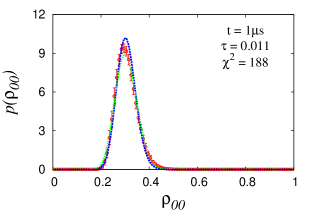
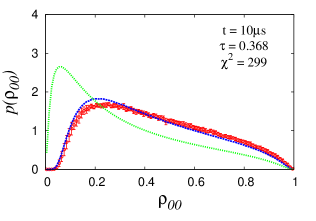
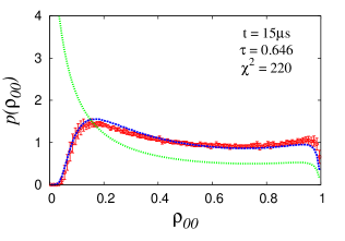
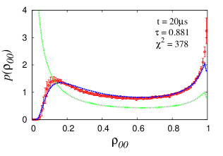
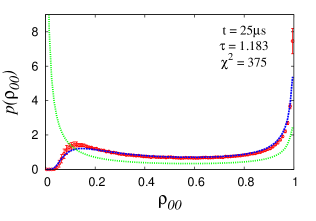
Figure 2: Evolution of the quantum trajectory distribution for the weak Z-measurement of a transmon, with the initial state $\rho_{00}=0.305(3)$. The histograms with bin width 0.01 (red) represent the experimental data for an ensemble of $10^{6}$ trajectories. The trajectory parameters (with errors) were $T_{1}=45(4)\mu s$, $\Delta t=0.5\mu s$, $I_{0}=128.44(2)$, $I_{1}=127.68(3)$, $\sigma=5.50(1)$. The blue curves are the best fits to the quantum diffusion model distribution including relaxation, with the evolution parameter $\tau\in[0,1.2]$; the green curves show the theoretical distributions with the same evolution parameter but with $T_{1}$ set to infinity.

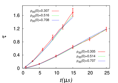
Figure 3: The best fit values of the time integrated measurement coupling $\tau$ for two values of the system-apparatus coupling, when experimental data for weak Z-measurement of a transmon with different initial states $\rho_{00}(0)$ are compared to the theoretical predictions. The stronger coupling (top curves) had $T_{1}=25(3)\mu s$, while the weaker coupling (bottom curves) had $T_{1}=45(4)\mu s$. It is obvious that $\tau$ is essentially independent of the initial state, and varies almost linearly with time after a slower initial build-up. The error bars (only some are shown for the sake of clarity) correspond to changes in $\tau$ that would change the $\chi^{2}$ values for the trajectory distribution fits by 100.

Our observed evolution of the quantum trajectory distribution, with the data divided into 100 histogram bins, is shown in Fig. 2, for a particular choice of the system-apparatus coupling and the initial qubit state. We have compared it with the simulated distribution of $10^{7}$ trajectories, obtained by integrating Eq.(6) with $\tau(g,t)$ as the only fit parameter. (We generated the simulated distributions for many values of $\tau$ to find the best fit, and we cross-checked that the simulated distributions agree with the solution of Eq.(7) obtained using a symmetric Trotter-type integration scheme.) This fitting of the entire trajectory distribution goes much beyond looking at just the mean and the variance of the distribution. With 100 data points and only one fit parameter, $\chi^{2}$ values less than a few hundred indicate good fits, and that is what we find. Also shown in Fig. 2 are the theoretically calculated trajectory distributions in absence of any relaxation, i.e. $T_{1}\rightarrow\infty$. We see that relaxation alters the distributions substantially, even for $t=0.1T_{1}$, and the quantum diffusion model of Eq.(4) successfully accounts for the changes.

We point out that the mismatch between theory and experiment grows with increasing evolution time, quite likely due to magnification of small initial uncertainties due to the iterative evolution. On closer inspection, we also observe certain systematic discrepancies, which are likely due to experimental imperfections that we have not accounted for. They include transients caused by photons left in the cavity after the initial heralding pulse, and contamination due to occupation of the higher excited states of the transmon drift . More stringent tests of the quantum diffusion model would need to control and account for them.

We have plotted the best fit $\tau$ values against $t$ in Fig. 3, for two values of the system-apparatus coupling and for different qubit initial states. It is seen that they are essentially independent of the initial state, supporting the assumption that the measurement evolution is governed by the system-apparatus coupling alone. Using different system-apparatus couplings and different transmon qubits, we have obtained similar results in the range $\tau(g,t)\in[0,2]$.

Discussion: We note that several investigations in recent years have observed quantum trajectories for transmons undergoing weak measurement; even the distribution of quantum trajectories has been qualitatively presented as grey-scale histograms in Ref. Weber . We have taken these observations to a quantitative level, demonstrating that the entire trajectory distribution can be described in terms of a single evolution parameter that is independent of the initial qubit state and the relaxation time. (Relaxation is unavoidable in any realistic evolution, and we accounted for it as a simple exponential decay.) This result puts on a strong footing the quantum diffusion paradigm, which replaces the projection postulate by an attraction towards the measurement eigenstates plus noise, both arising from the system-apparatus interaction with precisely related magnitudes. This unraveling of the measurement, singling out non-universal quantum diffusion as an appropriate extension of quantum mechanics, opens a window on to quantum physics beyond the textbook description. Also, each quantum trajectory with its noise history is associated with an individual experimental run, and understanding that can help in improving quantum control and feedback mechanisms Vijay .

Looking at quantum trajectories as physical processes has important implications. First is the construction of new physical observables from the distribution of quantum trajectories. The trajectories are highly constrained, with pure states ($\rho^{2}=\rho$, det$(\rho)=0$) remaining pure throughout measurement. With this restriction, any power-series expandable function $f(\rho)$ is a linear combination of $\rho$ and $I$, and so Tr$(f(\rho)O)$ reduces to ensemble averages that define conventional expectation values. Defining new physical observables that characterise the trajectory distribution is therefore a challenge.

Second, the fluctuation-dissipation relation for quantum trajectories is a powerful clue for understanding the dynamics of quantum measurement BornRule . The measurement is specific to each system-apparatus pair, with a particular value of interaction coupling and a particular type of noise. It implies that the quantum state collapse is not universal, and the environment can influence the measurement outcomes only via the apparatus and not directly.

Finally, while the quantum diffusion dynamics replaces the system-dependent Born rule by a system-independent noise, the origin of the noise remains to be understood. That necessitates making a quantum model for the apparatus. In our experiment, the apparatus pointer states are coherent states, with an inherent uncertainty equal to the zero-point fluctuations. They can provide the quantum noise for the trajectories through back-action. (The noise is quantum and not classical, because its inclusion makes the trajectory weights $w_{0},w_{1}$ in Eq.(5) go outside $[0,1]$ BornRule .) Understanding the irreversible quantum collapse would then amount to understanding why sufficiently amplified coherent states do not remain superposed Haroche . Amplification is a driven process, with built-in time asymmetry, and so the dynamics of the amplifier amplifrev would become a crucial ingredient for figuring out the quantum to classical cross-over. This is an open field for future explorations.

Acknowledgments: This work was supported by the Department of Atomic Energy of the Government of India. PK acknowledges a CSIR research fellowship from the Government of India. RV acknowledges funding from the Department of Science and Technology of the Government of India via the Ramanujan Fellowship.

Supplementary Information

.1 Experimental Details

The single junction 3D transmon device was fabricated using standard e-beam lithography and double angle evaporation of aluminum on an intrinsic silicon wafer. The device chip was placed inside a 3D aluminum cavity with a resonant frequency $\omega_{c}=7.240$ GHz and a linewidth $\kappa=3.05$ MHz. The chip was positioned away from the center of the cavity and the measured dispersive coupling was $g_{d}=81.76$ MHz. The qubit frequency was measured to be $\omega_{01}=4.93521$ GHz with an anharmonicity $\alpha=331.6$ MHz. The dispersive shift $\chi=365$ kHz is about an order of magnitude smaller than $\kappa$, so that the scattering phase shift and the average information per photon become small enough to enable operation in the weak measurement regime.

The Josephson Parametric Amplifier (JPA) is also fabricated using similar techniques, but it is designed with a SQUID to enable tuning of the amplifier center frequency. It is operated in the phase sensitive mode using double-pumping technique and amplifies only the quadrature containing the information about the $\sigma_{z}$ component of the qubit. The measurement pulse, paramp pump and the demodulation signal are all generated from the same microwave source, and variable attenuators and phase shifters are used to control each tone.

.2 Data Analysis

The observed variance of the measurement current distributions, $\sigma^{2}$, is modified from its ideal value due to limited amplifier efficiency: $\sigma^{2}=\sigma^{2}_{\rm ideal}+\sigma^{2}_{\rm noise}$. That affects the trajectory reconstruction, in the sense that the actual collapse is faster than what is seen. As a result, the fitted value of $\tau(g,t)$ automatically includes the factor of efficiency (the actual value of $\tau$ is different). Apart from this simple rescaling of $\tau$, limited amplifier efficiency has no other effect on comparison between the experimental data and the theoretical prediction. Working backwards (see ampeff ), we estimate the amplifier efficiency to be about $0.2$ for the weaker coupling, and about $0.35$ for the stronger coupling (for the same two data sets presented in Figs. 1,3).

The extracted values of $I_{0}$ and $I_{1}$ showed a noticeable anomalous behaviour in the first $2\mu s$; the former should be a constant and the latter should decay exponentially. This anomaly is likely due to the photons left in the cavity after the heralding/excitation pulse. To take care of it, we fitted the observed $I_{0}$ and $I_{1}$ by exponential functions for $t>2\mu s$. Then we constructed the evolution trajectories using the observed $I_{0}$ and $I_{1}$ for $t\leq 2\mu s$, and the fitted values of $I_{0}(t\rightarrow\infty)$ and $I_{1}(2.5\mu s)$ for $t>2\mu s$.

To obtain $\chi^{2}$ values for fits of the experimental quantum trajectory histograms with the theoretical predictions, we needed estimates of errors for the binned histogram values. With sufficiently large trajectory ensembles, the statistical errors are small compared to the systematic errors. The systematic errors were not directly available, because the histograms were produced after constructing the evolution trajectories as per Eqs.(9,11). So we first estimated errors in the parameters $T_{1}$, initial state, $I_{0}$, $I_{1}$ that are used in construction of the evolution trajectories. by direct analysis of the experimental data. Then we generated different trajectory ensembles by shifting the parameter values by their errors, one parameter at a time. Finally, assuming that the changes in histogram values obtained for individual parameter shifts were independent, they were added in quadrature to ascertain the total systematic error for the binned histogram values.

Overall, we have noticed that the agreement between experiment and theory improves with weaker couplings; we are yet to understand why. It may very well be that the unaccounted sources of error have a larger influence at stronger couplings.

References

- (1) J.A. Wheeler and W.H. Zurek (Eds.), Quantum Theory and Measurement (Princeton University Press, 1983).
- (2) V.B. Braginsky and F.Ya. Khalili, Quantum Measurement (Cambridge University Press, 1992).
- (3) D. Giulini, E. Joos, C. Kiefer, J. Kuptsch, I.-O. Stamatescu and H.D. Zeh, Decoherence and the Appearance of a Classical World in Quantum Theory (Springer, 1996).
- (4) H.M. Wiseman and G.J. Milburn, Quantum Measurement and Control (Cambridge University Press, 2010).
- (5) D. Bohm, A suggested interpretation of the quantum theory in terms of “hidden” variables. I. Phys. Rev. 85, 166-179 (1952); A suggested interpretation of the quantum theory in terms of “hidden” variables. II. Phys. Rev. 85, 180-193 (1952).
- (6) G. Ghirardi, Collapse Theories, The Stanford Encyclopedia of Philosophy, E.N. Zalta (ed.) (2011), [http://plato.stanford.edu/archives/win2011/entries/qm-collapse/].
- (7) R. Penrose, On gravity’s role in quantum state reduction. General Relativity and Gravitation 28, 581-600 (1996).
- (8) A. Bassi, K. Lochan, S. Satin, T.P. Singh and H. Ulbricht, Models of wave-function collapse, underlying theories and experimental tests. Rev. Mod. Phys. 85, 471-527 (2013).
- (9) B.S. DeWitt and N. Graham (Eds.), The Many-Worlds Interpretation of Quantum Mechanics, (Princeton University Press, 1973).
- (10) M. Gell-Mann and J.B. Hartle, Classical equations for quantum systems. Phys. Rev. D 47, 3345-3382 (1993).
- (11) C.A. Fuchs and B.C. Stacey, QBism: Quantum Theory as a Hero’s Handbook. arXiv:1612.07308[quant-ph] (2016).
- (12) A. Vinante, R. Mezzena, R. Falferi, M. Carlesso and A. Bassi, Improved non-interferometric test of collapse models using ultracold cantilevers. Phys. Rev. Lett. 119, 110401 (2017).
- (13) K.W. Murch, R. Vijay and I. Siddiqi, Weak measurement and feedback in superconducting quantum circuits. In Superconducting Devices in Quantum Optics, R. Hadfield and G. Johansson (Eds.), pp.163-185 (Springer, 2016).
- (14) P. Pearle, Reduction of the state vector by a nonlinear Schrödinger equation. Phys. Rev. D 13, 857-868 (1976); Towards explaining why events occur. Int. J. Theor. Phys. 18 489-518 (1979); Might God toss coins? Found. Phys. 12 249-263 (1982).
- (15) N. Gisin, Quantum measurements and stochastic processes. Phys. Rev. Lett. 52, 1657-1660 (1984); Stochastic quantum dynamics and relativity. Helvetica Physica Acta 62, 363-371 (1989).
- (16) L. Diósi, Quantum stochastic processes as models for state vector reduction. J. Phys. A: Math. Gen. 21, 2885-2898 (1988); Continuous quantum measurement and Itô formalism. Phys. Lett. A 129, 419-423 (1988).
- (17) A. Patel and P. Kumar, Weak Measurements, Quantum State Collapse and the Born Rule. Phys. Rev. A 96, 022108 (2017).
- (18) See for example: J. Bub, Interpreting the Quantum World, (Cambridge University Press, 1997). We do not use the concept of “weak values” at all.
- (19) K.W. Murch, S.J. Weber, C. Macklin and I. Siddiqi, Observing single quantum trajectories of a superconducting quantum bit. Nature 502, 211-214 (2013).
- (20) S.J. Weber, A. Chantasri, J. Dressel, A.N. Jordan, K.W. Murch and I. Siddiqi, Mapping the optimal route between two quantum states. Nature 511, 570-573 (2014).
- (21) A.N. Korotkov, Quantum Bayesian approach to circuit QED measurement. arXiv:1111.4016 (2011).
- (22) Only the diagonal elements of the density matrix determine the measurement outcomes, with . Eqs.(4,7) are simple modifications of the corresponding expressions in Ref. Gisin , to include effects of a finite . We follow the notation of Ref. BornRule .
- (23) This solution has been described in a path integral formalism in: A. Chantasri, J. Dressel and A.N. Jordan, Action principle for continuous quantum measurement. Phys. Rev. A 88, 042110 (2013); A. Chantasri and A.N. Jordan, Stochastic path-integral formalism for continuous quantum measurement. Phys. Rev. A 92, 032125 (2015).
- (24) For , 99% of the probability is within 1% of the two fixed points BornRule .
- (25) J. Koch, T.M. Yu, J. Gambetta, A.A. Houck, D.I. Schuster, J. Majer, A. Blais, M.H. Devoret, S.M. Girvin and R.J. Schoelkopf, Charge-insensitive qubit design derived from the Cooper pair box. Phys. Rev. A 76, 042319 (2007).
- (26) M. Hatridge, R. Vijay, D.H. Slichter, J. Clarke and I. Siddiqi, Dispersive magnetometry with a quantum limited SQUID parametric amplifier. Phys. Rev. B 83, 134501 (2011).
- (27) In our analysis, we checked that replacing Gaussians by cubic spline fits to the observed current distributions produces no discernible change in the results. The observed includes the effect of amplifier efficiency, as described in the Supplementary Information.
- (28) M. Hatridge, S. Shankar, M. Mirrahimi, F. Schackert, K. Geerlings, T. Brecht, K.M. Sliwa, B. Abdo, L. Frunzio, S.M. Girvin, R.J. Schoelkopf and M.H. Devoret, Quantum back-action of an individual variable-strength measurement. Science 339, 178-181 (2013).
- (29) J.E. Johnson, C. Macklin, D.H. Slichter, R. Vijay, E.B. Weingarten, J. Clarke and I. Siddiqi, Heralded state preparation in a superconducting qubit. Phys. Rev. Lett. 109, 050506 (2012).
- (30) The formal correspondence is .
- (31) We checked that adding a drift term to the simulated quantum trajectory distribution, i.e. violating the Born rule constraint , does not improve the fits.
- (32) R. Vijay, C. Macklin, D.H. Slichter, S.J. Weber, K.W. Murch, R. Naik, A.N. Korotkov and I. Siddiqi, Stabilizing Rabi oscillations in a superconducting qubit using quantum feedback. Nature 490, 77-80 (2012).
- (33) S. Deléglise, I. Dotsenko, C. Sayrin, J. Bernu, M. Brune, J.-M. Raimond and S. Haroche, Reconstruction of non-classical cavity field states with snapshots of their decoherence. Nature 455, 510-514 (2008).
- (34) A.A. Clerk, M.H. Devoret, S.M. Girvin, F. Marquardt and R.J. Schoelkopf, Introduction to quantum noise, measurement and amplification. Rev. Mod. Phys. 82, 1155-1208 (2010).