Ground-based detection of G star superflares with NGTS

Abstract

We present high cadence detections of two superflares from a bright G8 star (V = 11.56) with the Next Generation Transit Survey (NGTS). We improve upon previous superflare detections by resolving the flare rise and peak, allowing us to fit a solar flare inspired model without the need for arbitrary break points between rise and decay. Our data also enables us to identify substructure in the flares. From changing starspot modulation in the NGTS data we detect a stellar rotation period of 59 hours, along with evidence for differential rotation. We combine this rotation period with the observed ROSAT X-ray flux to determine that the star’s X-ray activity is saturated. We calculate the flare bolometric energies as $5.4^{+0.8}_{-0.7}\times 10^{34}$and $2.6^{+0.4}_{-0.3}\times 10^{34}$erg and compare our detections with G star superflares detected in the Kepler survey. We find our main flare to be one of the largest amplitude superflares detected from a bright G star. With energies more than 100 times greater than the Carrington event, our flare detections demonstrate the role that ground-based instruments such as NGTS can have in assessing the habitability of Earth-like exoplanets, particularly in the era of PLATO.

1 Introduction

Stellar flares are explosive phenomena caused by reconnection events in a star’s magnetic field (e.g. Benz & Güdel, 2010). When previously observed from the ground, they have been synonymous with active M stars, which flare regularly and brightly compared to their quiescent flux. Yet it is well known that the Sun shows regular flaring behaviour, with flares being detected over a wide range of energies. These range from $10^{23}$ erg for “nanoflares" (Parnell & Jupp, 2000) up to approximately $10^{32}$ erg for the largest occurrences such as the Carrington event (Carrington, 1859; Hodgson, 1859; Tsurutani et al., 2003). Observations of solar type stars, mainly with Kepler, have shown that much more energetic “superflares” of bolometric energies $10^{33}$ to $10^{36}$ erg are also possible (e.g. Shibayama et al., 2013).

The discovery of Earth sized exoplanets in the habitable zones of their host stars (e.g. TRAPPIST-1 and Proxima Centauri: Gillon et al., 2017; Anglada-Escudé et al., 2016) has given renewed importance to these superflares, in particular their effects on exoplanet habitability (e.g. Lingam & Loeb, 2017). Previous studies have found that the increase in UV radiation associated with flares can result in ozone depletion (Segura et al., 2010), changes to atmospheric composition (Venot et al., 2016) and even biological damage (e.g. Estrela & Valio, 2017). These effects are relatively well studied for M dwarf hosts, however it is expected that in future PLATO (Rauer et al., 2014) will reveal habitable zone planets around K and G stars. Compared to flares from later-type counterparts, detections of superflares from G stars are relatively rare. To date, no G star superflares have been detected with a CCD detector from the ground, although several have been seen either visually, in photography or with vidicon detectors (Schaefer, 1989; Schaefer et al., 2000).

In recent years, observations with the Kepler satellite (Borucki et al., 2010) have captured greater numbers of superflare events from G-type stars. These have been from both the long (30 minutes) and short (1 minute) cadence modes. In the long cadence mode, Maehara et al. (2012) and Shibayama et al. (2013) found 365 and 1547 superflares from 148 and 279 G-type stars respectively. In the 1-minute short cadence mode, 187 superflares from 23 solar-type stars were found by Maehara et al. (2015). From these detections, the statistical properties of superflares on G-type stars were considered, with Maehara et al. (2012) and Shibayama et al. (2013) finding a power law distribution of occurrence rate against energy of superflares that is comparable to solar flares, and with Maehara et al. (2015) identifying a correlation between the e-folding flare duration (time from flare amplitude peak to 1/e of its initial value) and the bolometric flare energy.

Candelaresi et al. (2014) also studied the occurrence rate of superflares from G dwarfs, as well as K and M dwarfs. They found the occurrence rate of superflares decreased with stellar effective temperature, and also peaked at a Rossby number of 0.1 (where Rossby number is the ratio of rotation period and convective turnover time). A Rossby number of 0.1 also corresponds to the rotation rate at which the X-ray emission of active stars saturates at 0.1 percent of the bolometric luminosity (e.g Pizzolato et al., 2003; Wright et al., 2011).

Previous studies have shown there may be a possible maximum limit on the energy that can be output by a G star superflare. Wu et al. (2015) identified a saturation value of around $2\times 10^{37}$ erg, using stars in the sample of Maehara et al. (2012) that displayed periodic modulation. Similar saturation behaviour was detected by Davenport (2016) from their sample of 4041 flaring stars, for example from the flaring G dwarf KIC 11551430. Davenport (2016) also found evidence for a weak correlation between flare luminosity and rotation period.

While these detections have shown the statistical properties of these white light flares, their temporal morphology and its link to solar flare morphology has not been investigated. This is due to undersampling of the flare rise and peak from previous stellar flare surveys (mainly Kepler), particularly for shorter duration events. High cadence (< 1 minute) data are required in order to compare observed solar flares and stellar superflares.

In this paper we present the first ground based CCD detections of superflares from a G type star. These are some of the most well resolved superflares to date, with a higher cadence than all Kepler measurements and most ground based observations. We present our measurements of the stellar and flare parameters and make comparisons with previously detected G star flares. We also present our modelling of each flare using a solar inspired general flare model.

Property	Value	Reference
$\textrm{RA}_{NGTS}$	03:08:34.9
$\textrm{Dec}_{NGTS}$	-21:13:22
$\textrm{RA}_{NGTS}$ (Deg)	47.14557
$\textrm{Dec}_{NGTS}$ (Deg)	-21.22284
$W4$	8.773	4
$W3$	9.699	4
$W2$	9.731	4
$W1$	9.699	4
$K_{s}$	9.768	1
$H$	9.865	1
$J$	10.216	1
$i^{\prime}$	11.174	3
$r^{\prime}$	11.356	3
$g^{\prime}$	11.899	3
Gaia $G$	11.354	2
$V$	11.562	3
$B$	12.291	3
$NUV$	16.943	5
$FUV$	20.666	5
ROSAT X-ray Count Rate (ct/s)	0.042	6
$\mu_{RA}$	$-1.2\pm 1.1$	7
$\mu_{DEC}$	$-6.2\pm 1.1$	7

Table 1: Properties of NGTS J0308-2113. Coordinates are given in the J2000 system. References are as follows, 1. Skrutskie et al. (2006), 2. Gaia Collaboration et al. (2016), 3. Henden & Munari (2014), 4.Cutri & et al. (2014), 5. Martin et al. (2005), 6. Boller et al. (2016) , 7. Zacharias et al. (2017) $NUV$, $FUV$, $i^{\prime}$, $r^{\prime}$, g’ are AB magnitudes. Proper motions are in mas/yr.

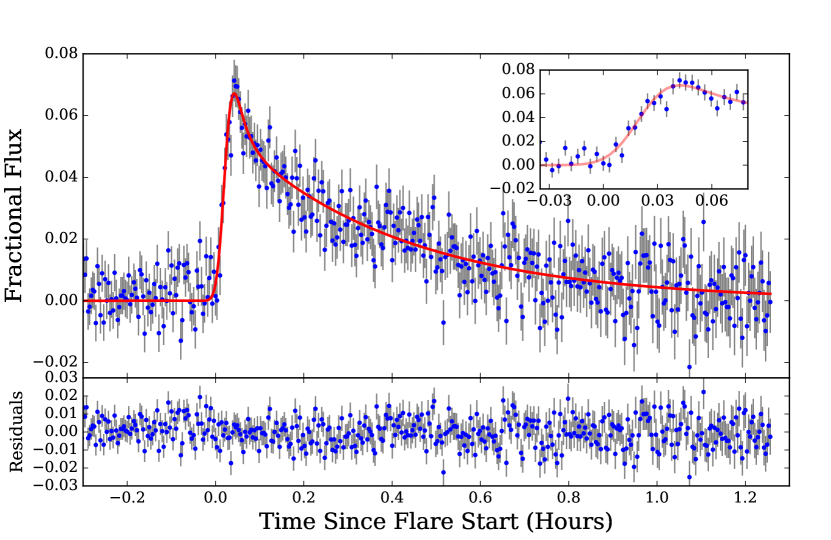
Figure 1: The superflare observed on NGTS J0308-2113  on 2016 January 3rd with best fitting model overlaid in red. The inset panel shows a zoomed in view of the data comprising the flare rise and peak, showing how the high cadence of NGTS has enabled us to resolve and fit to these regions. The bottom panel shows the residuals from our fitting. We note potential substructure in the flare decay around 0.7 hours and discuss this in Sect. 4.

2 Observations

The data presented in this paper were collected with the Next Generation Transit Survey (NGTS; Wheatley et al., 2017) over 80 nights between 2015 November 4th and 2016 February 25th. The two flares in this paper were detected on the nights of the 2015 December 17th and 2016 January 3rd. NGTS is a ground based transiting exoplanet survey, operating at Paranal. It has 12, 20 cm f/2.8, optical telescopes, each with a 520-890nm bandpass and exposure times of 10 seconds. Each single camera has a field of view of $\simeq$ 8 deg². NGTS is designed to monitor bright (I$\leq$16) K and M stars in the search for exoplanet transits (Wheatley et al., 2017). Unlike Kepler, NGTS observes without a set target list, meaning that all stars in our field of view that are bright enough can be studied. Each NGTS field is observed intensively whenever visible, and 3–4 fields are observed per telescope each year. With a total instantaneous field of view of 96 deg², and 10 s exposures, it is evident that NGTS is well suited to measure flare statistical distributions along with temporal morphology.

3 Data Analysis and Results

3.1 Flare search algorithm

When searching for flares, we started from the raw NGTS lightcurves and detrended them using a custom version of the sysrem algorithm (Mazeh et al., 2007). The full NGTS detrending is described by Wheatley et al. (2017). For these detrended lightcurves, we applied an additional filter to remove frames which showed excess variance above an empirically defined limit, primarily to remove data adversely affected by clouds. The timescale of stellar flares is minutes to hours (e.g. Poletto, 1989), so most flares will have durations less than one night, and we searched for flares on a night-by-night basis.

In order to find flares in each night, we searched for 3 consecutive points greater than 6 $MAD$ from the median of the night, where $MAD$ is the median absolute deviation. We have chosen $MAD$ as it is a robust measure of the variation within a night, and it is typically not strongly biased by the flare itself (a separate search is also carried out for flares that dominate the whole night). We applied no binning to the data, in order to fully utilise the time resolution of NGTS. Once the automated flagging procedure was complete, we inspected each flagged night visually and removed false positives. Examples of events which resulted in false positive flags include satellites passing through our aperture and high amplitude variable stars (e.g. RR Lyrae).

3.2 Flare detection

Using the method from Sect. 3.1 we detected a single flare, shown in Fig. 1, from the star NGTS J030834.9-211322  (NGTS J0308-2113). This star has also previously been identified as 2MASS J03083496-2113222. After identifying this flare we visually inspected each night to search for lower amplitude flares which were not flagged. From this, we identified a second flare, shown in Fig. 2.

To confirm the flares were not from a neighbouring source, we checked individual NGTS images from before and during the large flare, along with the positions of nearby stars from Gaia and 2MASS. The nearest source identified is from Gaia, a 20.658 magnitude star 10.5 arcseconds (2.1 pixels) away, placing it within our aperture. However, NGTS images reveal no shift in centroid position during the flare, and no light entering from outside the aperture, making us confident the flares are from NGTS J0308-2113.

3.3 Stellar Properties

To determine the stellar parameters for NGTS J0308-2113 we performed SED fitting using the broadband photometry listed in Tab. 1. These photometric values were obtained as part of the standard NGTS cross-matching pipeline (Wheatley et al., 2017). We use the SED modelling method described in Gillen et al. (2017), with the BT-SETTL and PHOENIX v2 model atmospheres. The SED fit is shown in Fig. 3. We see no IR-excess that might indicate NGTS J0308-2113 is a pre-main sequence star. From the SED fit we determine the effective temperature $T_{\rm eff}=5458\,^{+108}_{-85}$ K. We then use the information presented in Table 5 of Pecaut & Mamajek (2013) to identify the spectral type as G8. As a check on the spectral type we can also use the stellar colours with Tables 3 and 4 of Covey et al. (2007), which confirm the G8 spectral type. To determine the stellar radius, we assume the star is main sequence and use the empirical radius-temperature relation from equation 8 of Boyajian et al. (2012, 2017), determined from mass-radius calculations for 33 stars of spectral type between G5V and M5.5V. We calculate our stellar radius as 0.81 $\pm$ 0.04 R_☉. To estimate the uncertainty on the radius we use the median absolute deviation of 0.031 R_☉ from the Boyajian et al. (2012) fit and combine it with the upper error for our stellar temperature.

To check this source was not a giant star we compared the reduced proper motion, $H_{J}$ against $J-H$ colour (e.g. Gould & Morgan, 2003). Using the proper motion values from Tab. 1, we calculate $H_{J}$= -0.78 and $J-H$= 0.35. We use the criteria for dwarf/giant classification from Collier Cameron et al. (2007) to rule out the possibility this star is a giant.

We also note that this star was detected in X-rays with ROSAT. The detection of X-rays from this source is a sign of an active stellar corona (Boller et al., 2016).

3.4 Stellar Rotation

The NGTS lightcurve of NGTS J0308-2113 shows periodic flux variations, which we attribute to starspots moving across the visible disc of the star. We use this behaviour to determine the rotation period of the star, using a Lomb-Scargle periodgram. To do this, we use the astropy package LombScargle (Astropy Collaboration et al., 2013) and test for 20000 periods spaced between 13 seconds and 80 days. We mask the flares from our lightcurve when performing this analysis. Our periodogram for the whole time series of NGTS J0308-2113 is shown in Fig. 4, from which the period of the main peak is 59.09$\pm$0.01 hours (0.41 $d^{-1}$). We calculate the uncertainty on this period by fitting a sine wave to the data. Using the analysis from Baluev (2008) we determine the false alarm probability (FAP) of this peak to be negligible, a result of the high amount of data. We also note a second peak at 40 hours, which we found to be an alias by performing an identical Lomb Scargle analysis on a sine wave of period 59 hours with the same time sampling as our lightcurve.

This short spin period implies that NGTS J0308-2113 must be a relatively young star, most likely less than $\sim$600 Myr old, through comparing to the observed spin-age relations of open clusters (e.g. Sadeghi Ardestani et al., 2017; Douglas et al., 2017; Stauffer et al., 2016).

The amplitude of the observed spin modulation evolves with time. We split the lightcurve into three regions of activity, corresponding to an initial active portion, a secondary quiet portion and a final region where the amplitude increases once more. The 59 hour period phase folded data for these regions can be seen in Fig. 5.

Figure 2: A lower amplitude flare, from 2015 December 17th. The best fitting model is overlaid in red. We note the appearance of substructure at the flare peak and at 1.5 hours and discuss this in Sect. 4. The flare start time is given here by where the fit goes above 1 $\sigma$ above the quiescent flux, as discussed in Sect. 3.6.1

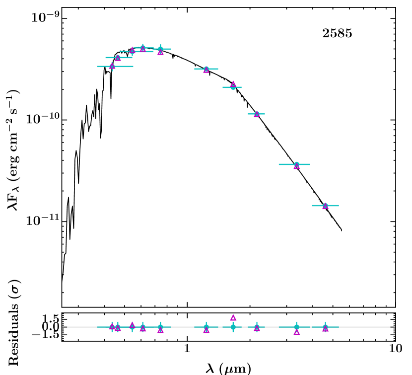
Figure 3: SED fit of NGTS J0308-2113 using the magnitudes listed in Tab. 1, matching best to a G8 spectral type.

Figure 4: Lomb-Scargle periodogram for our full lightcurve. Here we show frequencies between 0 and 2 day^-1. Note the 1 day alias of the peak groups. The largest peak corresponds to our detected 59 hour period.

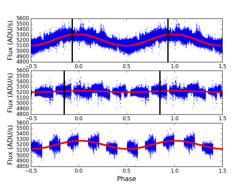
Figure 5: Phase folded data for the three regions of flux variation. Top is the initial active portion, middle is the quiet region and bottom is the following increase in activity. Overlaid in red is the sinusoidal fit for a 59 hour period. The black lines indicate the location of the small flare (top section) and the large flare (middle section).

Figure 6: Lomb-Scargle periodograms for each section shown in Fig. 5. Note the lack of a period detection in the quiescent region.

These regions are plotted in phase relative to the beginning of the lightcurve. The third region has a similar but slightly offset phase from the first, as well as less complete phase coverage due to a shorter duration. The durations of each region in the lightcurve are 40, 23 and 17 days respectively. The change in phase, along with the changing flux variation, can be explained by the decay of the original set of star spots and the formation of new ones. Starspot lifetimes have been studied by Bradshaw & Hartigan (2014) and for main sequence stars are on month timescales. One example is CoRoT-2, which has a starspot evolution timescale of 31$\pm$15 days (Silva-Valio & Lanza, 2011). Consequently we attribute our changing lightcurve modulation to starspot evolution.

We also searched for periodic signals separately in the three light curve regions. The three Lomb-Scargle periodograms are presented in Fig. 6. In the second, quiet, period of the light curve we see no evidence for periodic modulation. Calculating the modulation period of the third region gives a significantly longer rotation period of 60.87$\pm$0.04 hours (0.39 $d^{-1}$). This offset period suggests that the star exhibits differential rotation and that the new set of starspots are formed at a different latitude to the original active region.

We also check where each flare occurs in phase, to search for any relation to the location of the active region. The smaller flare occurs towards the end of the first region, close to maximum optical brightness, while the larger flare occurs in the second, quiet region at similar rotation phase (see Fig. 5). For the smaller flare, this is opposite in phase to the dominant active region. Neither flare seems to be located at a rotation phase where a large star spot group is obviously visible, and we discuss this further in Sect. 4.

3.5 X-ray Activity

As noted in Sect. 3.3, NGTS J0308-2113 has been detected in X-rays with ROSAT. The detection was made during the ROSAT all sky survey, and we adopt count rates and hardness ratios from the 2RXS catalog (Boller et al., 2016). The ROSAT PSPC count rate was $0.042\pm 0.018\,\rm s^{-1}$ and the hardness ratios in the standard ROSAT bands were HR1=$1.000\pm 0.325$ and HR2=$-0.428\pm 0.243$. The HR1 value indicates that the source was detected only in the ROSAT hard X-ray band (0.5–2.0 keV) and not in the soft band (0.1–0.4 keV).

The ROSAT PSPC count rate of NGTS J0308-2113 corresponds to a 0.1–2.4 keV energy flux of $5.7\times 10^{-13}\textrm{ erg s}^{-1}\textrm{cm}^{-2}$, using energy flux conversion factors determined for coronal sources by Fleming et al. (1995). This flux conversion uses the HR1 hardness ratio to account of the characteristic temperature of corona, and it has been applied to large samples of stars from the ROSAT all sky survey by Schmitt et al. (1995) and Huensch et al. (1998).

This X-ray flux corresponds to a 0.1–2.4 keV X-ray luminosity of $L_{X}=1.7\times 10^{30}\textrm{ erg s}^{-1}$ assuming a distance to NGTS J0308-2113 of 156 pc that we estimate using the apparent V magnitude and the expected absolute V magnitude for a G8V star (Gray & Corbally, 2009). Using the values for $T_{\rm eff}$ and $R_{*}$ from Sect. 3.3 we find the bolometric luminosity of the star to be $L_{Bol}=1.8\times 10^{33}\textrm{ erg s}^{-1}$ and hence $\log{L_{X}/L_{Bol}}=-3.1$, which corresponds to saturated X-ray emission (Pizzolato et al., 2003; Wright et al., 2011).

Combining this X-ray luminosity with our measurement of the stellar rotation period (Sect. 3.4), we can place NGTS J0308-2113 on the rotation-activity relation of Wright et al. (2011). This is shown in Fig. 7 where NGTS J0308-2113 can be seen to reside close to the break point between saturated X-ray emission and the power law decrease in activity to slower rotation. The Rossby number of 0.18 was calculated using our rotation period and the relation for convective turnover time from Wright et al. (2011).

Using the relation between the X-ray surface flux and average coronal temperature from Johnstone & Güdel (2015) we estimate an average coronal temperature of 10 MK. This is similar to the coronal temperature of 7.5 MK predicted from the rotation period using the relation by Telleschi et al. (2005).

The lack of detection of NGTS J0308-2113 in the ROSAT soft band, as well as its relatively large distance, suggests that it may be subject to stronger interstellar absorption than the sample of stars used to determine the flux conversion factors of Fleming et al. (1995). We therefore double checked our flux estimation using webpimms. We assumed a characteristic coronal temperature of 7.5 MK and an interstellar column density equal to the total Galactic columnn the direction of NGTS J0308-2113, which is $N_{\rm H}=2\times 10^{20}\,\rm cm^{-2}$ (Dickey & Lockman, 1990; Kalberla et al., 2005). The measured ROSAT PSPC count rate then corresponds to an unabsorbed 0.1–2.4 keV energy flux of $4.9\times 10^{-13}\,\rm erg\,cm^{-2}\,s^{-1}$, which is within 20 percent of our calculation using the flux conversion factors of Fleming et al. (1995).

Figure 7: Left: Stellar X-ray to bolometric luminosity ratio vs rotation period for NGTS J0308-2113 with the data from Wright et al. (2011). Right: Same, but for Rossby number. We have also overlaid the power law fit from Wright et al. (2011), with $\beta$=-2.18. NGTS J0308-2113 is shown here with a red star.

3.6 Flare Modelling

We model our flares following a similar method to Gryciuk et al. (2017), who fitted solar flares in soft X-rays. For both flares, we use the convolution of a Gaussian with a double exponential. A Gaussian is used to account for the heating in the flare rise, which has been found to be appropriate for solar flares (e.g. Aschwanden et al., 1998). A double exponential is used for the decay, accounting for thermal and non-thermal cooling processes, which has been used previously for the decay of stellar flares (e.g. Davenport et al., 2014). A convolution of these Gaussian and exponential functions is then analogous to the heating and cooling processes occurring during the flare (Gryciuk et al., 2017). With this physically motivated model we can utilise the high cadence of NGTS, in particular the flare rise which in the past has been fit using a polynomial or disregarded due to a lack of data points (e.g. Davenport et al., 2014; Pugh et al., 2016).

Before performing fitting, we inspected the full lightcurve and noted that several nights exhibited behaviour consistent with atmospheric extinction. We identified this trend by using the full lightcurve to fit for a first order atmospheric extinction term. This trend was then removed from the lightcurve, including the nights showing our flares. The nights before and after each flare were used to check the quality of this fit and were found to have the atmospheric extinction successfully removed. We also account for the flux modulation effects from starspots. To do this we use the preceding two and subsequent two nights and fit a sinusoid at the calculated 59 hour stellar rotation period. With this sinusoid we are able to remove any gradient due to rotation from the night. This is required most for the smaller flare, which sits in the first, more active region of the lightcurve (Sect. 3.4).

For both flares we perform fitting using an MCMC analysis with the python package emcee (Foreman-Mackey et al., 2013), using 500 walkers for 2000 steps and discarding the first 500 as a burn-in. During modelling we have increased our error bars to account for scintillation using the modified Young’s approximation with the empirical coefficient for Paranal (Young, 1967; Osborn et al., 2015). The best fitting models for the two flares are overlaid on Figs. 1 & 2. The best fitting parameters presented in Tab. 2.

3.6.1 Flare Amplitude and Duration

To determine the amplitude of each flare we use the maximum value of our fit. For the larger flare this gives a fractional amplitude of 6.9 per cent. For the smaller flare, using the value from the fit gives a fractional amplitude of 1.2 per cent. Inspecting Fig. 2, there appears to be impulsive substructure at the flare peak, which is not accounted for in our model. Taking the average of the five data points around the peak gives an peak amplitude of 2.0$\pm$0.3 per cent.

To obtain a measure of the full duration of the flare, we again make use of our fit. We define the start and end of the flare as the points where the model rises and then falls more than 1$\sigma$ above the background flux level, as in Gryciuk et al. (2017). Here $\sigma$ is determined from the quiescent flux before the flare. From this, we determine the flare duration of the larger flare to be 55 minutes. Due to the decreased amplitude to error ratio of the smaller flare, we do not calculate the full flare duration using this method. However, we also calculate the flare duration with two additional methods - using its e-folding timescale (as performed in Shibayama et al., 2013) and its scale time (the duration where the flare is above half the maximum flux value). Again, we use our fit for these. For the large and small flare, we calculate the e-folding timescale as 16 and 55.5 minutes respectively, and the scale time as 11 and 42 minutes respectively. With our fit we can also calculate the timescale of the flare rise, using the time from the flare start to the peak of the model. Using this, we calculate the flare rise time as 2.5 minutes for the larger flare. If we use the 1 $\sigma$ start limit for the smaller flare, we estimate the flare rise as at least 7.4 minutes.

Property	Large	Small
Energy (erg)	$5.4^{+0.8}_{-0.7}\times 10^{34}$	$2.6^{+0.4}_{-0.3}\times 10^{34}$
Fit Amplitude (per cent)	6.9	1.2
Full Duration (min)	55	N/A
e-folding duration (min)	16	55.5
Scale time (min)	11	42
Flare rise (min)	2.5	>7.4

Table 2: Properties of each superflare detected from NGTS J0308-2113.

3.7 Flare Energy

The method used to calculate the flare energy is based on that described by Shibayama et al. (2013), and makes the assumption that the flare and star act as blackbody radiators, with the flare having a blackbody spectrum of temperature 9000 $\pm$ 500 K in order to estimate the flare luminosity. Using the stellar effective temperature and radius from Sect. 3.3, we calculate the bolometric energy of the larger and smaller flare to be $5.4^{+0.8}_{-0.7}\times 10^{34}$ erg and $2.6^{+0.4}_{-0.3}\times 10^{34}$ erg respectively. It is striking that the smaller flare is only a factor two less energetic despite having an amplitude around six times lower. Comparing to the Carrington event energy of $\approx$ $10^{32}$ ergs (Tsurutani et al., 2003), we can see that each flare had a bolometric energy several hundred times greater than this.

From a total of 422 hours of observation for this star, we have detected two flares. We can use this measurement to estimate the flaring rate for flares above $2.6^{+0.4}_{-0.3}\times 10^{34}$ erg as approximately 40 per year.

4 Discussion

4.1 Flare Properties

We have detected two superflares from the G star NGTS J0308-2113 with high-cadence NGTS optical photometry. These are the first ground-based CCD detections of superflares from a G star. Our NGTS observations have much higher cadence than the Kepler flare detections, allowing us to resolve the flare rise and substructure.

The larger flare is shown in Fig. 1 and was calculated to have a bolometric energy of $5.4^{+0.8}_{-0.7}\times 10^{34}$erg and a fractional amplitude of 6.9 per cent. Due to the increased time resolution of our measurements compared to almost all previous superflare detections, we have been able to fit this flare with a physically-motivated model that includes a Gaussian pulse to describe the impulsive flare rise (as employed previously for solar flares). For the decay, our data require two exponential components. Separate impulsive and gradual decay components been seen previously in some stellar flares, and attributed to decay of blackbody-like emission and chromospheric emission respectively (Hawley et al., 2014; Kowalski et al., 2013). We can also see that this flare displays a flattening around the peak, or a “roll-over”. Similar flare peak behaviour has been seen by Kowalski et al. (2011) from ULTRACAM observations of the dM3.5e star EQ Peg A. This behaviour is captured in the fitted model as a result of the observed combination of Gaussian heating and exponential cooling. Further, we can identify smaller peaks in the decay of the flare, located at approximately 0.7 and 1.0 hour after the flare start in Fig.  1. Structure, or “bumps”, such as this have been previously identified in flare decays with Kepler (e.g Balona et al., 2015).

Our model has also been used to fit the smaller flare of NGTS J0308-2113, shown in Fig. 2. This flare has a much lower relative amplitude of just 1.2 per cent, making it the lowest-amplitude G star flare to have been detected from the ground. Despite its low amplitude, this smaller flare has a much slower rise and longer duration than the larger flare (by factors of 3–4) so that it has a high total energy of $2.6^{+0.4}_{-0.3}\times 10^{34}$erg, which is only a factor 2 lower than the larger flare. When fitting this smaller flare it became apparent that there was additional structure at the flare peak. This can be seen in the residuals of Fig. 2, as a small spike lasting approximately one minute. This is a sign of an additional heating pulse at the end of the initial flare rise. In this flare we also detect subtructure around 1.5 hours after the flare start (visible in the residuals). The amplitude of the peak at this time is approximately 1 per cent, which is comparable with the amplitude of the main flare. Considering the timing of this substructure relative to the main flare peak, it is likely an example of sympathetic flaring (e.g. Moon et al., 2002).

One advantage of our flare model, combining a Gaussian heating pulse with exponential cooling, is that it avoids an arbitary discontinuity between the end of the rise and the beginning of the decay. This has generally not been the case with previous stellar flare models, which have tended to include an instantaneous transition between functions describing the rise and decay (e.g. Davenport et al., 2014). Our model also provides a well-defined measure of the rise timescale, allowing for studies of how the flare rise time changes between flares. In this case we see the lower amplitude flare rising much more slowly than the high amplitude example. This highlights how wide-field high-cadence surveys such as NGTS can contribute to the quantitative characterisation of stellar flares.

4.2 Starspots and Flare Phases

Our analysis of the NGTS light curve of NGTS J0308-2113 revealed a 59.09$\pm$0.01 h periodic modulation that we interpret the changing visibility of starspots on the stellar rotation period (Sect. 3.4). The initial set of starspots appear to decay during the observations, and no spin modulation is detected for an interval of around 23 d. Periodic modulation begins again towards the end of the NGTS observations, and at a slightly longer period, suggesting that the star exhibits differential rotation and that new starspots have emerged at a different latitude.

Checking where the flares occur in rotation phase reveals that the smallest flare occurs in antiphase to the dominant starspot group, while the larger flare occurs during the quiescent interval of the lightcurve (at a similar spin phase to the first flare). These flare timings are perhaps surprising, as we might expect to see superflares when large active regions are present and visible. Instead, our results suggest that the observed superflares do not emerge from the dominant active regions on the stellar surface. Such behaviour is not unprecedented, as observations of the M dwarfs AD Leo and GJ 1243 showed no correlation between stellar flare occurrence and rotational phase (Hunt-Walker et al., 2012; Hawley et al., 2014). A similar result was found for the K dwarf KIC 5110407, with all but the two strongest flares showing no correlation with the most active regions (Roettenbacher et al., 2013). In these cases it was suggested that the dominant active region might be located at the pole, such that it is always in view and flares can be seen at any spin phase. An alternative is that the majority of flares originate from smaller spot groups that do not cause the dominant flux modulation.

4.3 Comparison with Kepler

In Fig. 8 we compare the superflares of NGTS J0308-2113 with G star superflares detected with Kepler. We use the samples from Shibayama et al. (2013) and Maehara et al. (2015) for the long and short cadence Kepler data respectively. NGTS J0308-2113 has a Kepler magnitude of 11.4, calculated using the stellar g’ and r’ magnitudes and Eqn. 2a from Brown et al. (2011). This magnitude makes it one of the brightest G stars seen to exhibit a superflare (see Fig. 8). The larger flare from NGTS J0308-2113 also has a greater amplitude than all but one of those detected in short cadence Kepler data. This flare also has a shorter duration than most detected with Kepler. This comparison demonstrates that NGTS has a sufficiently wide-field of view and high photometric precision to detect rare and interesting stellar flares from bright stars. Each flare is also observed with higher cadence than has previously been possible.

Figure 8: Comparison of the fractional amplitudes and Kepler magnitude of our flares from NGTS J0308-2113 (red stars) with G star superflares detected in short cadence (black squares) and long cadence (black crosses) Kepler data. When comparing fractional amplitudes between NGTS and Kepler  it should be noted that the Kepler bandpass extends blueward of NGTS.

4.4 X-ray Activity

Thanks to the relative proximity and hence brightness of NGTS J0308-2113 we were able to measure its X-ray luminosity using archival ROSAT data (Sect. 3.5). We found that the star is in the saturated X-ray regime, with $\log L_{X}/L_{Bol}=-3.1$, and that its X-ray emission is consistent with the rotation activity relation of Wright et al. (2011). It was not detected in the ROSAT soft X-ray band, likely due to interstellar absorption. Using our measured spin period and the relation for convective turnover time by Wright et al. (2011) we estimated the Rossby number of NGTS J0308-2113 to be 0.18. Interestingly, this places the star close to the peak of superflare occurrence rates found by Candelaresi et al. (2014).

We can also compare the X-ray luminosity of NGTS J0308-2113 with that of other G stars exhibiting superflares. Yabuki et al. (2017) found nine stars with X-ray detections from the Kepler superflare sample of Shibayama et al. (2013). Using these nine X-ray detections they identified a correlation between the largest white-light flare energies (estimated from Kepler data) and quiescent $L_{X}$ with

$$E_{Bol}\propto L_{X}^{1.2\pm^{0.3}_{0.4}}.$$ (1)

Based on this relation, we would expect NGTS J0308-2113 to exhibit flares of energies up to approximately $8\times 10^{35}$ erg. This is around 13 times greater than the energy of our larger flare, suggesting NGTS J0308-2113 sometimes exhibits even more energetic flares than the examples we have detected with NGTS.

4.4.1 Maximum Flare Energy

An alternative method to estimate the potential maximum flare energy is to use the starspot activity. This is done using equation (1) from Shibata et al. (2013),

$$E_{flare}\approx 7\times 10^{32}(\textrm{erg})\bigg{(}\frac{f}{0.1}\bigg{)}\bigg{(}\frac{B}{10^{3}\textrm{G}}\bigg{)}^{2}\bigg{(}\frac{A_{\textrm{spot}}}{3\times 10^{19}\textrm{cm}^{2}}\bigg{)}^{3/2}$$ (2)

where $f$, $B$ and $A_{\textrm{spot}}$ are the fraction of magnetic energy that can be released as flare energy and the magnetic field strength and area of the starspot respectively. We estimate the starspot area from the lightcurve modulation normalised by the average brightness, following the method of Notsu et al. (2013). We use the region of greatest brightness variation to estimate the area, obtaining a value equivalent to 0.04 of the visible stellar surface. We assume $f$=0.1 (Aschwanden et al., 2014) and $B$=1000 - 3000G (typical comparison values for solar-type stars e.g. Solanki, 2003; Maehara et al., 2015) and calculate $E_{flare}=0.9-8.5\times 10^{35}$erg. This estimated value is the same order of magnitude as that calculated from the X-ray data, predicting a flare of greater energy than our largest event.

4.5 Implications For Exoplanet Habitability

Understanding the properties of superflares from G stars is important when considering the habitability of Earth-like exoplanets, including those expected to be detected with PLATO (Rauer et al., 2014). Stellar flares are known to be associated with intense ultraviolet radiation (e.g. Stelzer et al., 2006; Tsang et al., 2012), which can reduce levels of atmospheric ozone (e.g. Lingam & Loeb, 2017) and damage the DNA of biological organisms (e.g. Castenholz & Garcia-Pichel, 2012). Associated X-ray and extreme-ultraviolet radiation can also erode the planetary atmosphere and drive water loss. Stellar flares are also associated with Coronal Mass Ejections (CMEs), and while planetary magnetospheres may protect against the quiescent stellar wind, CMEs can act to compress the magnetosphere and expose the planetary atmosphere to further erosion and dessication (e.g. Kay et al., 2016; Lammer et al., 2007).

The detections of superflares presented in this paper demonstrate that wide-field ground-based surveys such as NGTS are capable of characterising the rates and energies of superflares from G-type stars, despite their relatively low fractional amplitude. Since flare detections with ground-based telescopes can be made and announced in real time it may also be possible to trigger immediate follow up of superflares with larger narrow-field telescopes while the flares are still in progress. This has not been possible to date due to the unpredictable nature of superflares and inevitable delays in downlinking and processing data from space telescopes such as Kepler. Real-time follow up of NGTS flares might then provide the multi-wavelength observations needed to assess the impact of superflares on potentially habitable exoplanet atmospheres.

5 Conclusions

In this work we have presented the detection of two superflares from the G8 star NGTS J030834.9-211322 using NGTS. These are the first G star superflares detected from the ground using a CCD, and they are among the highest cadence measurements of any superflares to date. We fit both flares with a model that incorporates a Gaussian heating pulse, as seen previously in solar flares, and exponential decay on two timescales. The model fit provides the amplitude, energy and duration of each flare, and we find the two flares have similar total energies despite their different amplitudes and durations. The larger flare has an unusually high amplitude and short duration for a G star superflare. Our model also allows us to measure the timescale of the flare rise, an interval that has been undersampled in previous studies, and we find the longer duration flare has a slower rise. We have also detected substructure in both flares.

The stellar rotation period of NGTS J0308-2113 was measured to be 59 hours, and we found evidence for differential rotation. The X-ray luminosity of the star was calculated to be $1.7\times 10^{30}\textrm{ erg s}^{-1}$, with $\log{L_{X}/L_{Bol}}=-3.1$ implying saturated X-ray emission, as expected for a G8 star with such a short spin period. The Rossby number of 0.18 places NGTS J0308-2113 close to the peak of the occurence rate distribution implied by previous flare detections.

Our results highlight the potential for wide-field ground-based surveys such as NGTS to determine the rates, energies and morphologies of superflares from G stars, despite the modest white-light amplitudes of such flares. Further detections and real-time multi-wavelength follow up will be important in assessing the habitability of Earth-like exoplanets around G stars, including those to be found with PLATO.

References

- Anglada-Escudé et al. (2016) Anglada-Escudé G., et al., 2016, Nature, 536, 437
- Aschwanden et al. (1998) Aschwanden M. J., Dennis B. R., Benz A. O., 1998, ApJ, 497, 972
- Aschwanden et al. (2014) Aschwanden M. J., Xu Y., Jing J., 2014, ApJ, 797, 50
- Astropy Collaboration et al. (2013) Astropy Collaboration et al., 2013, A&A, 558, A33
- Balona et al. (2015) Balona L. A., Broomhall A.-M., Kosovichev A., Nakariakov V. M., Pugh C. E., Van Doorsselaere T., 2015, MNRAS, 450, 956
- Baluev (2008) Baluev R. V., 2008, MNRAS, 385, 1279
- Benz & Güdel (2010) Benz A. O., Güdel M., 2010, ARA&A, 48, 241
- Boller et al. (2016) Boller T., Freyberg M. J., Trümper J., Haberl F., Voges W., Nandra K., 2016, A&A, 588, A103
- Borucki et al. (2010) Borucki W. J., et al., 2010, Science, 327, 977
- Boyajian et al. (2012) Boyajian T. S., et al., 2012, ApJ, 757, 112
- Boyajian et al. (2017) Boyajian T. S., et al., 2017, ApJ, 845, 178
- Bradshaw & Hartigan (2014) Bradshaw S. J., Hartigan P., 2014, ApJ, 795, 79
- Brown et al. (2011) Brown T. M., Latham D. W., Everett M. E., Esquerdo G. A., 2011, AJ, 142, 112
- Candelaresi et al. (2014) Candelaresi S., Hillier A., Maehara H., Brandenburg A., Shibata K., 2014, ApJ, 792, 67
- Carrington (1859) Carrington R. C., 1859, MNRAS, 20, 13
- Castenholz & Garcia-Pichel (2012) Castenholz R. W., Garcia-Pichel F., 2012, in , Ecology of Cyanobacteria II. Springer, pp 481–499
- Collier Cameron et al. (2007) Collier Cameron A., et al., 2007, MNRAS, 380, 1230
- Covey et al. (2007) Covey K. R., et al., 2007, AJ, 134, 2398
- Cutri & et al. (2014) Cutri R. M., et al. 2014, VizieR Online Data Catalog, 2328
- Davenport (2016) Davenport J. R. A., 2016, ApJ, 829, 23
- Davenport et al. (2014) Davenport J. R. A., et al., 2014, ApJ, 797, 122
- Dickey & Lockman (1990) Dickey J. M., Lockman F. J., 1990, ARA&A, 28, 215
- Douglas et al. (2017) Douglas S. T., Agüeros M. A., Covey K. R., Kraus A., 2017, ApJ, 842, 83
- Estrela & Valio (2017) Estrela R., Valio A., 2017, preprint, (arXiv:1708.05400)
- Fleming et al. (1995) Fleming T. A., Molendi S., Maccacaro T., Wolter A., 1995, ApJS, 99, 701
- Foreman-Mackey et al. (2013) Foreman-Mackey D., Hogg D. W., Lang D., Goodman J., 2013, PASP, 125, 306
- Gaia Collaboration et al. (2016) Gaia Collaboration et al., 2016, A&A, 595, A2
- Gillen et al. (2017) Gillen E., Hillenbrand L. A., David T. J., Aigrain S., Rebull L., Stauffer J., Cody A. M., Queloz D., 2017, preprint, (arXiv:1706.03084)
- Gillon et al. (2017) Gillon M., et al., 2017, Nature, 542, 456
- Gould & Morgan (2003) Gould A., Morgan C. W., 2003, ApJ, 585, 1056
- Gray & Corbally (2009) Gray R. O., Corbally J. C., 2009, Stellar Spectral Classification
- Gryciuk et al. (2017) Gryciuk M., Siarkowski M., Sylwester J., Gburek S., Podgorski P., Kepa A., Sylwester B., Mrozek T., 2017, Sol. Phys., 292, 77
- Hawley et al. (2014) Hawley S. L., Davenport J. R. A., Kowalski A. F., Wisniewski J. P., Hebb L., Deitrick R., Hilton E. J., 2014, ApJ, 797, 121
- Henden & Munari (2014) Henden A., Munari U., 2014, Contributions of the Astronomical Observatory Skalnate Pleso, 43, 518
- Hodgson (1859) Hodgson R., 1859, MNRAS, 20, 15
- Huensch et al. (1998) Huensch M., Schmitt J. H. M. M., Voges W., 1998, A&AS, 132, 155
- Hunt-Walker et al. (2012) Hunt-Walker N. M., Hilton E. J., Kowalski A. F., Hawley S. L., Matthews J. M., 2012, PASP, 124, 545
- Johnstone & Güdel (2015) Johnstone C. P., Güdel M., 2015, A&A, 578, A129
- Kalberla et al. (2005) Kalberla P. M. W., Burton W. B., Hartmann D., Arnal E. M., Bajaja E., Morras R., Pöppel W. G. L., 2005, A&A, 440, 775
- Kay et al. (2016) Kay C., Opher M., Kornbleuth M., 2016, ApJ, 826, 195
- Kowalski et al. (2011) Kowalski A. F., Mathioudakis M., Hawley S. L., Hilton E. J., Dhillon V. S., Marsh T. R., Copperwheat C. M., 2011, in Johns-Krull C., Browning M. K., West A. A., eds, Astronomical Society of the Pacific Conference Series Vol. 448, 16th Cambridge Workshop on Cool Stars, Stellar Systems, and the Sun. p. 1157 (arXiv:1103.0822)
- Kowalski et al. (2013) Kowalski A. F., Hawley S. L., Wisniewski J. P., Osten R. A., Hilton E. J., Holtzman J. A., Schmidt S. J., Davenport J. R. A., 2013, ApJS, 207, 15
- Lammer et al. (2007) Lammer H., et al., 2007, Astrobiology, 7, 185
- Lingam & Loeb (2017) Lingam M., Loeb A., 2017, preprint, (arXiv:1708.04241)
- Maehara et al. (2012) Maehara H., et al., 2012, Nature, 485, 478
- Maehara et al. (2015) Maehara H., Shibayama T., Notsu Y., Notsu S., Honda S., Nogami D., Shibata K., 2015, Earth, Planets, and Space, 67, 59
- Martin et al. (2005) Martin D. C., et al., 2005, ApJ, 619, L1
- Mazeh et al. (2007) Mazeh T., Tamuz O., Zucker S., 2007, in Afonso C., Weldrake D., Henning T., eds, Astronomical Society of the Pacific Conference Series Vol. 366, Transiting Extrapolar Planets Workshop. p. 119 (arXiv:astro-ph/0612418)
- Moon et al. (2002) Moon Y.-J., Choe G. S., Park Y. D., Wang H., Gallagher P. T., Chae J., Yun H. S., Goode P. R., 2002, ApJ, 574, 434
- Notsu et al. (2013) Notsu Y., et al., 2013, ApJ, 771, 127
- Osborn et al. (2015) Osborn J., Föhring D., Dhillon V. S., Wilson R. W., 2015, MNRAS, 452, 1707
- Parnell & Jupp (2000) Parnell C. E., Jupp P. E., 2000, ApJ, 529, 554
- Pecaut & Mamajek (2013) Pecaut M. J., Mamajek E. E., 2013, ApJS, 208, 9
- Pizzolato et al. (2003) Pizzolato N., Maggio A., Micela G., Sciortino S., Ventura P., 2003, A&A, 397, 147
- Poletto (1989) Poletto G., 1989, Sol. Phys., 121, 313
- Pugh et al. (2016) Pugh C. E., Armstrong D. J., Nakariakov V. M., Broomhall A.-M., 2016, MNRAS, 459, 3659
- Rauer et al. (2014) Rauer H., et al., 2014, Experimental Astronomy, 38, 249
- Roettenbacher et al. (2013) Roettenbacher R. M., Monnier J. D., Harmon R. O., Barclay T., Still M., 2013, ApJ, 767, 60
- Sadeghi Ardestani et al. (2017) Sadeghi Ardestani L., Guillot T., Morel P., 2017, MNRAS, 472, 2590
- Schaefer (1989) Schaefer B. E., 1989, ApJ, 337, 927
- Schaefer et al. (2000) Schaefer B. E., King J. R., Deliyannis C. P., 2000, ApJ, 529, 1026
- Schmitt et al. (1995) Schmitt J. H. M. M., Fleming T. A., Giampapa M. S., 1995, ApJ, 450, 392
- Segura et al. (2010) Segura A., Walkowicz L. M., Meadows V., Kasting J., Hawley S., 2010, Astrobiology, 10, 751
- Shibata et al. (2013) Shibata K., et al., 2013, PASJ, 65, 49
- Shibayama et al. (2013) Shibayama T., et al., 2013, ApJS, 209, 5
- Silva-Valio & Lanza (2011) Silva-Valio A., Lanza A. F., 2011, A&A, 529, A36
- Skrutskie et al. (2006) Skrutskie M. F., et al., 2006, AJ, 131, 1163
- Solanki (2003) Solanki S. K., 2003, A&ARv, 11, 153
- Stauffer et al. (2016) Stauffer J., et al., 2016, AJ, 152, 115
- Stelzer et al. (2006) Stelzer B., Schmitt J. H. M. M., Micela G., Liefke C., 2006, A&A, 460, L35
- Telleschi et al. (2005) Telleschi A., Güdel M., Briggs K., Audard M., Ness J.-U., Skinner S. L., 2005, ApJ, 622, 653
- Tsang et al. (2012) Tsang B. T. H., Pun C. S. J., Di Stefano R., Li K. L., Kong A. K. H., 2012, ApJ, 754, 107
- Tsurutani et al. (2003) Tsurutani B. T., Gonzalez W. D., Lakhina G. S., Alex S., 2003, Journal of Geophysical Research: Space Physics, 108, n/a
- Venot et al. (2016) Venot O., Rocchetto M., Carl S., Roshni Hashim A., Decin L., 2016, ApJ, 830, 77
- Wheatley et al. (2017) Wheatley P. J., et al., 2017, preprint, (arXiv:1710.11100)
- Wright et al. (2011) Wright N. J., Drake J. J., Mamajek E. E., Henry G. W., 2011, ApJ, 743, 48
- Wu et al. (2015) Wu C.-J., Ip W.-H., Huang L.-C., 2015, ApJ, 798, 92
- Yabuki et al. (2017) Yabuki K., Tsuboi Y., Sasaki R., Sugawara Y., Katsuda S., Maehara H., 2017, in Serino M., Shidatsu M., Iwakiri W., Mihara T., eds, 7 years of MAXI: monitoring X-ray Transients, held 5-7 December 2016 at RIKEN. Online at <A href=“https://indico2.riken.jp/indico/conferenceDisplay.py?confId=2357”> https://indico2.riken.jp/indico/conferenceDisplay.py?confId=2357</A>, p.187. p. 187
- Young (1967) Young A. T., 1967, AJ, 72, 747
- Zacharias et al. (2017) Zacharias N., Finch C., Frouard J., 2017, AJ, 153, 166