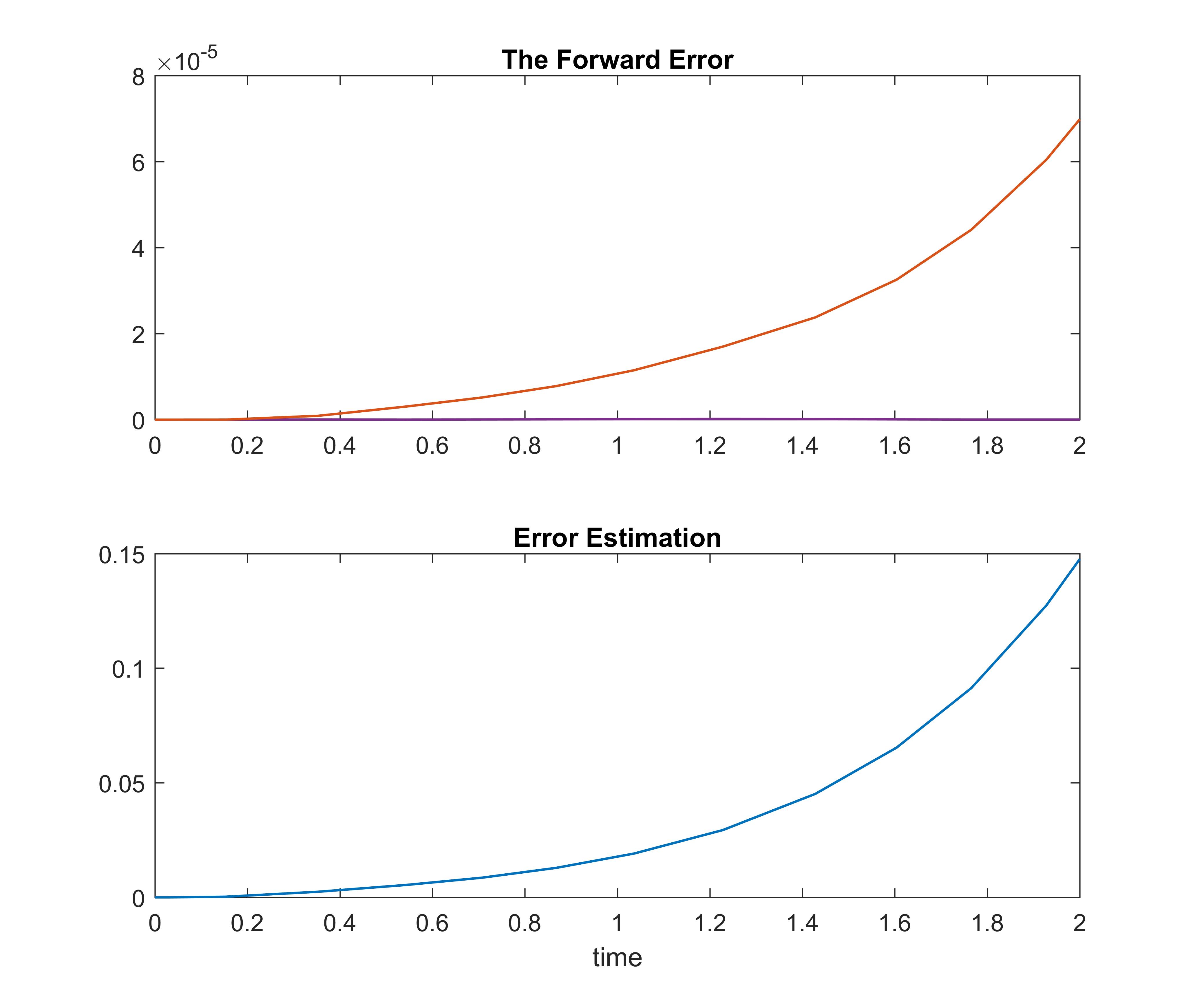
he error estimation boundary will be very huge. However, this phenomenon does not indicate that error estimation is not reliable, in contrast, it works well. We will use Example LABEL:ex:1 to explain this situation. As we know, in Example LABEL:ex:1, the exact solution is $x^{*}=e^{t}$, if there is an error $\varepsilon$ in numerical solution, satisfying $\widetilde{x}(t)=(1+\varepsilon)e^{t}-\varepsilon$. The residual will easily be calculated as $\delta(t)=\varepsilon$. Moreover, the forward error is $\Delta x=x^{*}-\widetilde{x}=\varepsilon(1-e^{t})$. It’s obviously that the forward error of this example will be inevitable exponential growth, no matter what solver you choose. By Theorem LABEL:thm:main, as $\lambda_{1}=1$ and $h_{max}=0$ , our error estimation $\varepsilon(e^{t}-1)$ is also exponential increasing and exactly same as the forward error boundary $\|\Delta x\|_{\infty}$. It means that in general it is a sharp bound and it is difficult to improve this bound.

1 Examples

In order to show performance of our error estimation to IVPS of Linear ODEs, in this section, we firstly use Theorem LABEL:thm:main to deal with a time-invariant system example. Then we give a time-variant stable system example. At last, we provide a time-variant unstable example from automobile suspension system with an adjustable damping model.

1.1 Time-invariant System Example

Consider this initial-value problem:

$${\bm{x}}(t)^{\prime}={\bm{A}}{\bm{x}}(t)+{\bm{q}}(t),{\bm{A}}=\left(\begin{array}[]{cc}-1&0\\ 0&2\end{array}\right),{\bm{x}}(0)=0.$$

In order to get the exact solution easily, let ${\bm{x}}=(cos(\pi t)-1,sin(\pi t))$. Then we obtain $\bf{q}=\bf{x}^{\prime}-\bf{A}\cdot\bf{x}$. Draw a figure by MATLAB as follow, in which the forward error $\Delta x_{1}(t)$ (the blue curve) almost is stable to fluctuate around zero, the forward error $\Delta x_{2}(t)$ (the red curve) is inevitable exponential growth. Our method of error estimation is exponential growth too, and it does gives an upper bound of the forward error all the time. Note, in our examples, we choose $\delta_{max}$ at each step and $h_{max}$ over the period.

Figure 1: Time-invariant System Error Estimation

1.2 A Time-variant Stable System Example

Consider there is a linear dynamic system, its relationship as follow:

$$\bf{A}(t)=\left(\begin{array}[]{cc}-6+0.2\cdot sin(2\pi t)&0\\ 1&-5-0.1\cdot sin(\pi t)\end{array}\right)\ \mbox{ and }{\bm{x}}=\left(\begin{array}[]{c}cos(\pi t)-1\\ sin(\pi t)\end{array}\right)$$

In order to get the exact solution, we suppose the relationship $\bf{q}=\bf{x}^{\prime}-\bf{A}(t)\cdot\bf{x}$. At the period $t\in[0,6]$, it’s clear the initial ${\bm{x}}(0)=\left(\begin{array}[]{c}0\\ 0\end{array}\right)$. We first use ode$45$ to solute the ODEs, we can get the numerical solution. Secondly, to deal with the numerical solution by hermit cubic spline, it’s easy to calculate the residual of numerical solution. Finally, according to theorem 3.3, we can do error estimation of numerical solution and draw a figure as Fig.(2).

Figure 2: A Time-variant Stable System Error Estimation

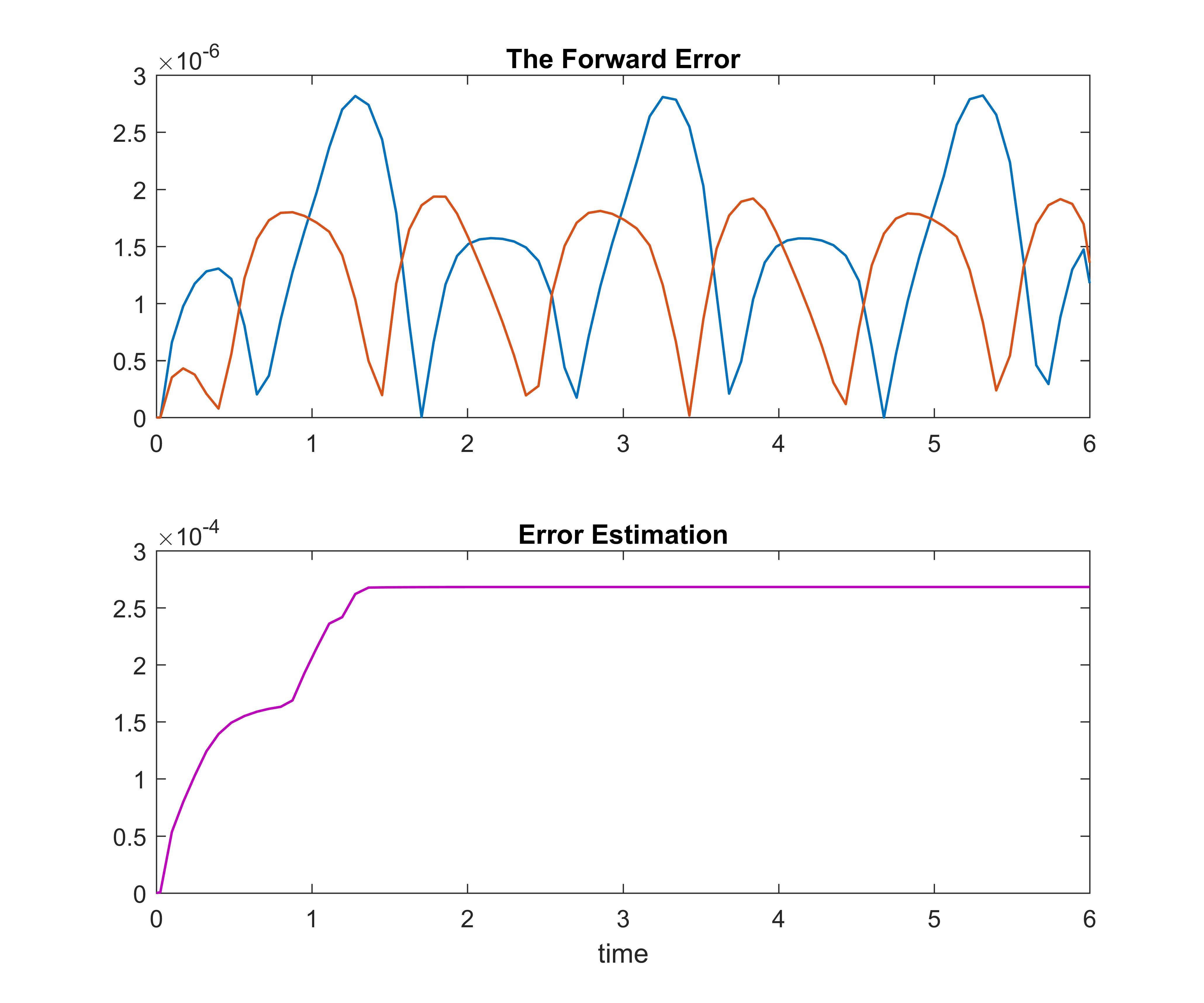
In this figure, we can see the boundary of error estimation is almost bigger than the boundary of forward error all the time. And both of them are stable as to the system is stable.

1.3 Automobile Suspension System with an Adjustable Damping Absorber

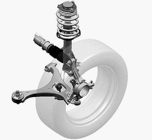
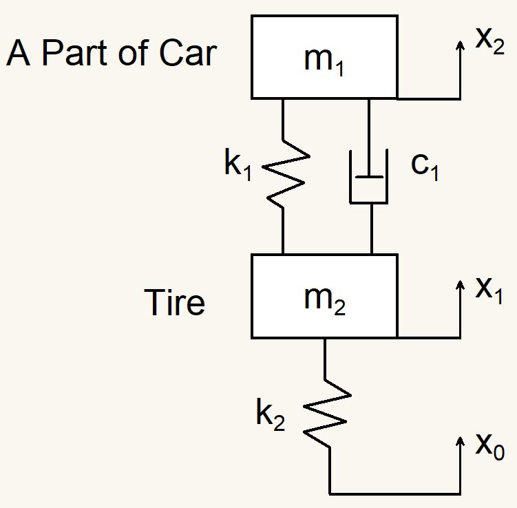
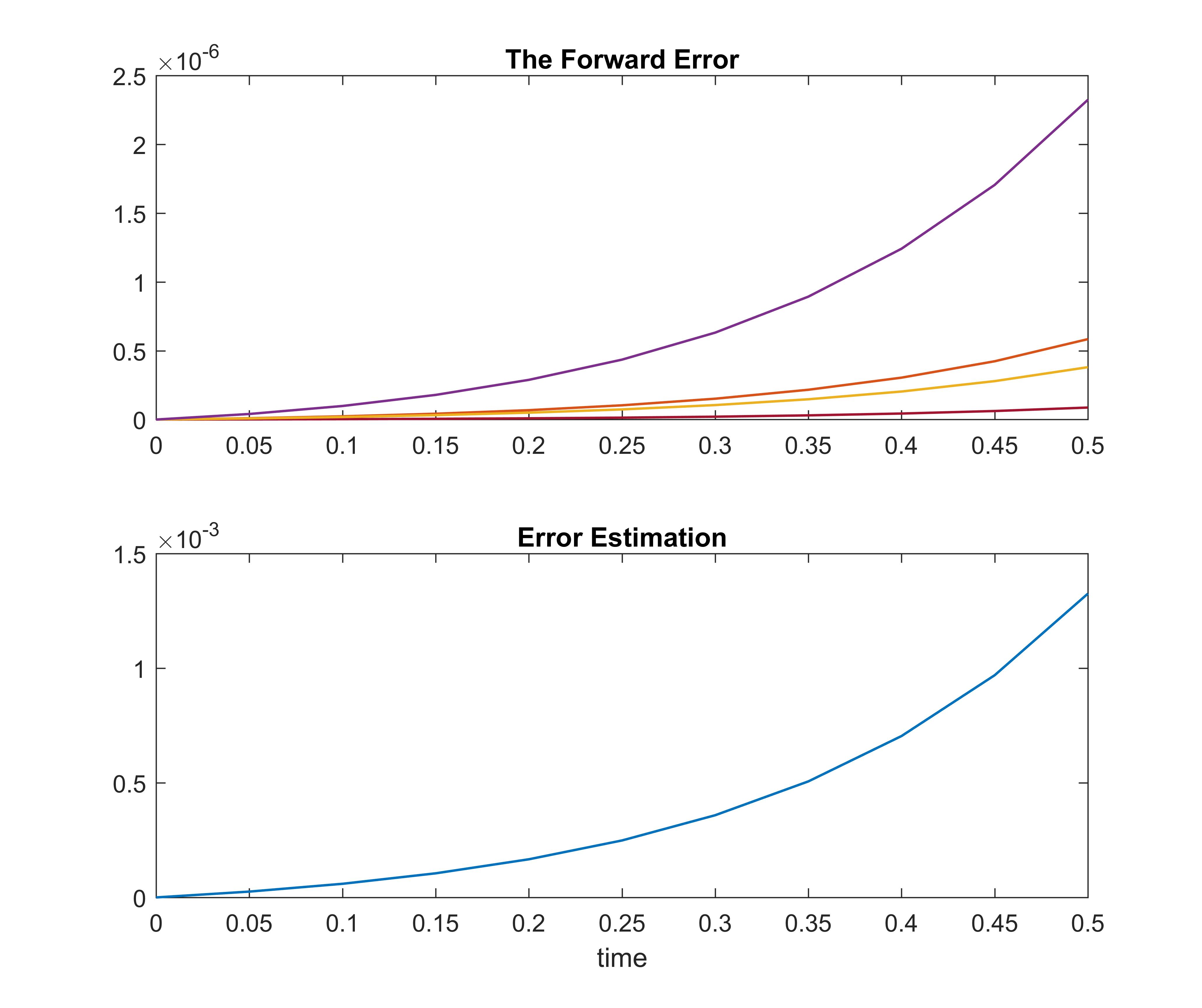
While a car go though a ramp, we want it smooth enough, usually we use computer aided engineering software to simulate and to predict movement trends. However, the numerical solution of this dynamic system has error, which feedback to control-system will bring catastrophic result. It’s necessary to calculate the forward error of numerical solution in order to warn control-system.The following we give an example of error estimation to automobile suspension system. Suppose: in the vertical direction, part mass of car $m1=500kg$, shock-absorbing spring $k1=1500N/m$, the mass of tire $m2=100kg$, the elasticity coefficient of tire $k2=2000N/m$.Additionally, almost automobiles on road have active suspension, that’s to say the damping will be changed by control system. Suppose the damping is changed as $c1=200+200\cdot cos(2\pi t)N\cdot m/s^{2}$ in our example. The ODEs of this system can be write as $\bf{x}^{\prime}=\bf{A}(t)\cdot\bf{x}+\bf{q}$. Where $\bf{x}=\left(\begin{array}[]{c}x_{1}\\ x_{1}^{\prime}\\ x_{2}\\ x_{2}^{\prime}\end{array}\right)$ are part of car’s displacement and velocity, tire’s displacement and velocity, respectively. While go though a ramp, during $t\in[0,0.5]$, our goal is $\bf{x}=\left(\begin{array}[]{c}0.1\cdot sin(\pi t)\\ 0.1\cdot\pi cos(\pi t)\\ 0.01\cdot sin(\pi t)\\ 0.01\cdot\pi cos(\pi t)\end{array}\right)$, and initial value is $\bf{x}(0)=\left(\begin{array}[]{c}0\\ 0.1\cdot\pi\\ 0\\ 0.01\cdot\pi\end{array}\right)$, moreover, we can get $\bf{q}=\bf{x}^{\prime}-\bf{A}(t)\cdot\bf{x}$.

Figure 3: Automobile Suspension System

By using Taylor expansion $cos(x)=1-\frac{1}{2!}x^{2}+o(x^{2})$, we can get

$$\bf{A}(t)=\left(\begin{array}[]{cccc}0&1&0&0\\ 3&\frac{4}{5}-\frac{\pi^{2}\cdot t^{2}}{250}&-3&\frac{\pi^{2}\cdot t^{2}}{250}-\frac{4}{5}\\ 0&0&0&1\\ \frac{\pi^{2}\cdot t^{2}}{50}-4&15&35&4-\frac{\pi^{2}\cdot t^{2}}{50}\\ \end{array}\right)$$

As to the automobile suspension system is a time-variant unstable system, the forward error of numerical solution exponential growth by time, it’s the same as the error estimation. That’s to say, to unstable system ,if we need error estimation accuracy enough, the time should be short enough.

Figure 4: Automobile Suspension System

2 Conclusion

In this paper, we give a definition of residual, which accurately passes each point of a numerical solution. It has a tight relationship with the forward error. Although, as indicated in Theorem LABEL:thm:cubicHermiterror, the Hermite cubic spline has error, the forward error satisfies the ODE (LABEL:eq:forward_error_solution) by Lemma LABEL:lem:forward. For error estimation, we give a bound of time-invariant or time-variant system without exact solution. The bound of the estimation mainly depends on biggest eigenvalue, often smaller than Lipschitz constant. Verified by examples, our estimation method has better performance in unstable system. Moreover, if the backward error of numerical solution is smaller, that’s to say the numerical solver is better or it uses a smaller step size, the error estimation will be more accurate accordingly.

3 Acknowledgement

This work was partially supported by NSFC 11471307 and CAS Research Program of Frontier Sciences (QYZDB-SSW-SYS026).

References

- [1] Wolfgang Walter. Ordinary Differential Equations. Springer, New York, 1998.
- [2] Uri M. Ascher, Linda R. Petzold. Computer Methods for Ordinary Differential Equations and Differential Equations and Differential-algebraic Equations. SIAM, Phaladephia, 1998.
- [3] Robert M.corless, Nicolas Fillion. A Graduate Introduction to Numerical Methods. Springer, 2013.
- [4] Endre Süli, David Mayers. An introduction to numerical analysis. Cambridge Unibersity Press, Cambridge, 2003.
- [5] Gene H.Golub, Charles F.Van Loan. Matrix Computations. The Johns Hopkins Unibersity Press, New York, 2012.
- [6] L.F. Shampine. Error Estimation and Control for ODEs. Journal of Scientific Computing, 2005, 25(1-2):3-16.
- [7] W.H.Enright. Continuous Numerical Methods for ODEs with Defect Control. Journal of Computational and Applied Mathematics, 2000, 125:159-170.
- [8] L.F.Shampine. Solving ODEs and DDEs with Residual Control. Applied Numerical Mathematics, 2005, 52(1):113-127.
- [9] D.J.Higham. Robust Defect Control with Runge-Kutta Schemes. Siam Journal on Numerical Analysis, 1989, 26(5):1175-1183.
- [10] D.J.Higham. Runge CKutta Defect Control Using Hermite-Birkhoff Interpolation. Siam J.sci.statist.comput, 1991, 12(5):991-999.
- [11] J.R.Dormand, P.J.Prince. Global Error Estimation with Runge-Kutta Methods. Ima Journal of Numerical Analysis, 1984, Anal.4:169-184.
- [12] J.R.Dormand, P.J.Prince. Global Error Estimation with Runge-Kutta Methods II. Ima Journal of Numerical Analysis, 1985, Anal.5:481-497.
- [13] L.F.Shampine, H.A.Watts. Global Error Estimation for Ordinary Differential Equations. ACM Transactions on Mathematical Software, 1976, 2(2):172-186.
- [14] L.F.Shampine, H.A.Watts. Algorithm 504, GERK: Global Error Estimation for Ordinary Differential Equations. ACM Transactions on Mathematical Software, 1976, 2(2):200-203.
- [15] M.C.Calvo, D.J.Higham, J.I.Montijano, andL Rández. Stepsize Selection for Tolerance Proportionality in Explicit Runge CKutta Codes. Advances in Computational Mathematics, 1997, 7(3):361-382.
- [16] L.F.Shampine. Tolerance Proportionality in ODE Codes. Springer Berlin Heidelberg, Berlin, 1989.
- [17] H.J.Stetter. Tolerance Proportionality in ODE-codes. Humboldt University Press, März, 1980.
- [18] W.H.Enright. A New Error Ccontrol for Initial Value Solvers. Applied Mathematics and Computation, 1989, 31(1):288-301.