Evaluating the role of data quality when sharing information in
hierarchical multi-stock assessment models, with an application to dover
sole
Samuel D. N. Johnson (corresponding), Sean P. Cox,
School of Resource and Environmental Management, Simon Fraser University, 8888 University Drive, BC, Canada,
Abstract
An emerging approach to data-limited fisheries stock assessment uses hierarchical multi-stock assessment models to group stocks together, sharing information from data-rich to data-poor stocks. In this paper, we simulate data-rich and data-poor fishery and survey data scenarios for a complex of dover sole stocks. Simulated data for individual stocks were used to compare estimation performance for single-stock and hierarchical multi-stock versions of a Schaefer production model. The single-stock and best performing multi-stock models were then used in stock assessments for the real dover sole data. Multi-stock models often had lower estimation errors than single-stock models when assessment data had low statistical power. Relative errors for productivity and relative biomass parameters were lower for multi-stock assessment model configurations. In addition, multi-stock models that estimated hierarchical priors for survey catchability performed the best under data-poor scenarios. We conclude that hierarchical multi-stock assessment models are useful for data-limited stocks and could provide a more flexible alternative to data-pooling and catch only methods; however, these models are subject to non-linear side-effects of parameter shrinkage. Therefore, we recommend testing hierarchical multi-stock models in closed-loop simulations before application to real fishery management systems.
Introduction
Fisheries stock assessment modeling uses catch and abundance monitoring data to estimate the status and productivity of exploited fish stocks (Hilborn 1979). Despite improvements in catch monitoring and increasing prevalence and quality of fishery-independent surveys of abundance, many fisheries remain difficult to assess because the data lack sufficient statistical power to estimate key quantities necessary for management (Peterman 1990). Low power data may arise, for example, because time-series are short relative to the productivity cycles of exploited fish stocks, historical fishing patterns may be weak or uninformative, and monitoring data may simply be too noisy to extract biomass and productivity signals (Magnusson and Hilborn 2007). Where these situations occur, stocks are often deemed data-limited (MacCall 2009, Carruthers et al. 2014).
An emerging approach to fisheries stock assessment is to use a hierarchical approach to assess data-limited stocks simultaneously with data-rich stocks. Data-limited stocks can “borrow information” from data-rich stocks, providing a compromise between data-intensive single-stock assessments and problematic data-pooling approaches (Jiao et al. 2009, 2011, Punt et al. 2011). The hierarchical multi-stock approach, which shares information between data-rich and data-poor stocks, treats multiple stocks of the same species as replicates that, to varying degrees, share environments, life history characteristics, ecological processes, and fishery interactions (Peterman et al. 1998, Punt et al. 2002, Malick et al. 2015). Information present in the observations for data-rich replicates is shared with more data-poor replicates via hierarchical prior distributions on parameters of interest (Punt et al. 2011, Thorson et al. 2015). Sharing information in this way could improve scientific defensibility of assessments for data-limited stocks, because stock status and productivity estimates are informed by data rather than strong a priori assumptions on population dynamics parameters.
Information-sharing properties of hierarchical models are realized as the shared hierarchical priors induce shrinkage of estimated parameters towards the overall prior mean (Carlin and Louis 1997, Gelman et al. 2014). Although shrinkage can reduce bias in the presence of high uncertainty (e.g. very data-limited stocks), it may also increase bias for data-rich replicates by pulling estimated parameters closer to the group mean. Shrinkage properties are well understood for hierarchical linear models (James and Stein 1961, Raudenbush and Bryk 2002), including those applied in fisheries. For example, when estimating productivity of Pacific salmon stocks, hierarchical Ricker stock-recruitment models are more successful at explaining variation in stock productivity when stocks are grouped at scales consistent with climatic variation (Peterman et al. 1998, Mueter et al. 2002). It is unclear, however, whether the benefits observed for linear models extend to iteroparous groundfish stocks, for which productivity parameters are deeply embedded within non-linear population dynamics and statistical models.
Parameter shrinkage has been observed in stock assessments for data-limited groundfish and shark species when grouped with data-moderate species (Jiao et al. 2009, 2011, Punt et al. 2011), but it is unknown whether such shrinkage in reality increases or decreases bias in parameter estimates. Simulation tests of the hierarchical multi-stock approach to age-structured assessments revealed that bias reductions in one species often induce greater bias for others in the assessment group, indicating that shrinkage could imply unwanted trade-offs (Punt et al. 2005).
In this paper, we used a simulation approach to investigate relationships between hierarchical model structure, bias, and precision for hierarchical multi-stock Schaefer stock assessment models. For the hierarchical multi-stock models, we defined shared prior distributions on survey catchability and optimal harvest rate (productivity) and then identified combinations of shared priors that produced the most reliable estimates of key management parameters when fit to simulated data from high and low data quality multi-stock complexes. Best performing singl and multi-stock models were then applied to real data for a dover sole complex in British Columbia, Canada.
Methods
We simulated a multi-stock complex representing the dover sole (Microstomus Pacificus) fishery in British Columbia, Canada. Dover sole stocks were simulated under low to high data quality (statistical power) scenarios. Under each scenario, bias and precision metrics were determined for key management parameters under both single-stock and hierarchical multi-stock Schaefer models. In our hierarchical multi-stock assessment models shared evolutionary history and a common scientific survey influenced our choice of shared prior distributions. For example, stocks that share evolutionary history may have similar productivity at low stock sizes (Jiao et al. 2009, 2011), and a common trawl survey may induce correlations in catchability (trawl efficiency) observation errors.
Study system
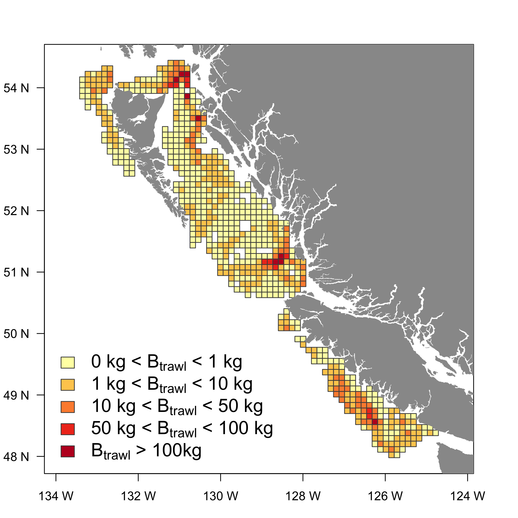
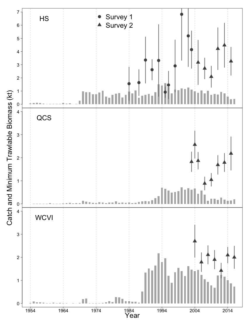
British Columbia’s dover sole complex is divided into three distinct but connected stocks (Figure 1), distributed along the BC coast from the northern tip of Haida Gwaii, south through Hecate Strait into Queen Charlotte Sound, and on the west coast of Vancouver Island. Although the dover sole fishery has operated since 1954, prior to 1970 it was very limited, increasing to present levels by the late 1980’s (Figure 2).
Despite a long history of exploitation, dover sole stocks have never been evaluated using model-based assessments. No observational data exists for the Queen Charlotte Sound (QCS) and west coast of Vancouver Island (WCVI) stocks prior to 2003, precluding a model based assessment before that time (Fargo 1999). The Haida Gwaii and Hecate Strait (HS) stock was surveyed from 1984 - 2003 (Figure 2, Survey 1), but data was only used to perform catch curve analyses for total mortality rate estimates (Fargo 1998). During 1984 - 2003, a fine-mesh trawl survey was used for the Vancouver Island stock and a portion of the Hecate Strait stock, but the survey was not designed for groundfish and produced stock indices that were highly variable. Since 2003, a new bottom trawl survey has operated coast-wide, which samples all three stocks (Figure 2, Survey 2), but no assessment has been performed in that time.
Dover sole may be suitable for a hierarchical multi-stock assessment for 3 main reasons. First, the Hecate Strait stock has longer series of informative data than the other stocks, potentially providing information for the other two stocks. Second, modeling a single-species makes it likely that stock productivities and responses to the environment are similar. Lastly, all stocks are observed by Survey 2, making it likely that the observation model parameters for each stock are similar for that survey. By applying the hierarchical multi-stock approach, the similarities between stocks may be exploited to the benefit of the whole complex, extending model based stock assessments for dover sole for the first time.
Simulation Framework
Our simulation framework was composed of an operating model that simulated biological dynamics, catch, and observational data, and an assessment model that performed both single-stock and hierarchical multi-stock assessments from the simulated data. Both operating and assessment models used a process-error Schaefer formulation for biomass dynamics, where the biomass in each year is deviated from the expected value using a log-normal process error term. This choice allowed us to focus on the effects of hierarchical estimation and shrinkage without confounding among hierarchical priors and the model structure. We used the R statistical software package to specify the operating model, and the Template Model Builder (TMB) package to specify the assessment model (Kristensen et al. 2015, R Core Team 2015).
The simulation approach is described below in 3 main sections (i) the operating model, (ii) assessment models, and (iii) simulation experiments. The next section describes the operating model structure, including process errors, and how catch and survey observations were generated. Assessment models are then outlined, with details of the shared hierarchical prior distributions given in the supplemental material. Finally, we present the experimental design and performance metrics for the simulations.
Operating model
We simulated biomass dynamics for each stock in our assessment complex on an annual time step , using the process-error Schaefer model (Punt 2003)
| (1) |
where is the biomass of stock at time , is the intrinsic rate of increase, is the unfished equilibrium biomass, and is the process error deviation for stock at time . Schaefer model process error deviations were decomposed via the sum of a shared (across stocks) mean year-effect , and a correlated (among stocks) stock-specific effect , which is the component of the vector , that is,
We specified the covariance matrix as the diagonal decomposition , where is a diagonal matrix of stock-specific standard deviations , and is the matrix of stock correlations. For simplicity, we simulated all stocks with identical pair-wise covariances, i.e., for a 3 stock complex
and all stocks experienced the same magnitude of stock-specific process errors where , implying
The operating model values of and were chosen to give a total process error variance of , or roughly a 10% total relative standard error (Table 1).
We simulated 34 years of fishery history from 1984 () to 2017 (). Each stock was initalized in 1984 at a pre-determined depletion level relative to unfished biomass, i.e., . Unless otherwise stated, we set , which is varied as an experimental factor (Table 2). Because we simulated a single-species, multi-stock complex, we used the same base biological parameters kilo-tonnes, and for all stocks (Table 1). While identical parameters may not adequately represent the true dover sole complex, it helped us focus on the effects of shrinkage in parameter estimates, rather than differences in biological parameters. This choice also simplified reporting and interpretation of the results, allowing us to focus on parameter estimates for a smaller set of representative stocks, rather than analysing every stock in the complex.
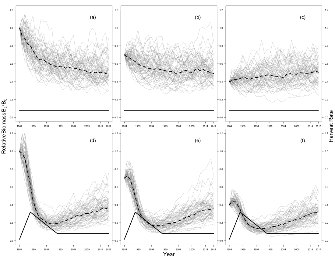
Fishery catch and fishery independent biomass indices were sampled from each stock each year. We simulated perfectly implemented catch , where was the harvest rate applied in a pulse fishing event following each year’s production. We also assumed that catch was fully observed (i.e., no under-reporting). Harvest rates were simulated in three temporal phases and scaled to optimal fishing mortality as , where is the piecewise linear function of :
| (2) |
where , and are the initial, development, and managed phase harvest rates, respectively, is the last time step of the development phase, and is the beginning of the final managed phase (Figure 3). In the base operating model, we used values , and for harvest rate multipliers, with (1988), and (1998) for phase timing, to simulate a high initial development phase followed by a reduction in pressure, allowing the stock to recover. This formulation was designed to create more and less informative catch histories, depending on the parameter values (Schnute and Richards 1995).
Survey indices of biomass were simulated for each stock and survey via the observation model
where is stock-specific catchability coefficient for survey . Observation errors were simulated via the distribution
where is the survey observation error log scale standard deviation for survey . Within each survey, stock-specific catchabilities were randomly drawn from a log-normal distribution with a mean survey catchability coefficient and between-stock log-standard deviation via
It is not always the case that catchability will be correlated closely between stocks. Indeed, we were able to model catchability as a correlated process between stocks because we used swept area biomass estimates as our stock indices. To see this, note that the general formula for catchability is , where is gear efficency, is the average area fished by the gear during the survey, and is the total area of the surveyed stock’s habitat (Arreguı’n-Sánchez 1996). Because the geographic boundaries of stocks may differ, it will usually be the case that between 2 distinct stocks and , even if the average surveyed area and gear efficiency are the same. For a trawl survey, it is advantageous that the area swept by the fishing gear is often known exactly, with , where is the standard tow duration, is the tow velocity and is the door-width of the trawl net. Therefore, the total of randomly sampled survey catches from a total effort of tows can be transformed into biomass estimates when scaled by the reciprocal of the proportion of area swept, e.g. . Then the effect of stock area is scaled out of the index, and catchability is reduced to gear efficency , or the response of individual fish to the survey gear. We then assumed that this response is similar between individuals of the same species. This calculation extends to swept area biomass estimates calculated from a stratified survey, like the trawl survey used for Dover Sole.
We simulated biomass indices from two surveys operating over different periods to emulate the current dover sole complex history (Figure 2). The first () represented Survey 1, which operated from 1984 to 2003 (), with observation model parameters for the observation errors, and a mean survey catchability of with a standard deviation of . For survey 2 (), which operated from 2003 to 2017 (), we modeled an observation error standard deviation of , and a mean catchability of with a standard deviation of .
Assessment model
We estimated stock-specific biological and management parameters using multi-stock and single-stock versions of a state-space Schaefer stock assessment model. We minimized the effect of assessment model mis-specification by matching the deterministic components of the biomass dynamics in the assessment models and the operating model, Equation (1). Details of the assessment model prior distributions are not presented in this section. Instead, the equations for each multi-level prior in the hierarchical multi-stock assessment model are given in Table 3, and the details of all prior distributions are given in supplementary material S1.
Hierarchical multi-stock assessment models
For the full hierarchical multi-stock model, we defined shared prior distributions on (1) conditional maximum likelihood estimates of stock-specific catchability within each survey and (2) optimal harvest rate , which was used as a surrogate for stock productivity (Table 3). In total, we defined 4 configurations, including a “null” multi-stock model. Each multi-stock model configuration was defined by whether each of the hierarchical priors was estimated along with the leading model parameters. When a hierarchical prior was “off”, shared priors were bypassed and the model used the fixed hyperprior mean and standard deviation instead (Table 3, Single level priors). Full details of the single and multi-level priors are in supplemental material.
Single-stock assessment model
The single-stock assessment model was defined as a special case of the multi-stock null model. Prior distributions on catchability and productivity were the single level priors (Table 3, q.4 and U.4).
Optimization
Assessment models applied the Laplace approximation to integrate the objective function over random effects, obtaining a marginalized likelihood (Kristensen et al. 2015). The marginalized likelihood was then maximized via the nlminb() function in R to produce parameter estimates and corresponding asymptotic standard errors (R Core Team 2015). We considered an assessment model converged when the optimisation algorithm reported convergence, which was characterized by gradient components of the TMB model all having magnitude less than 0.0001, and a positive definite Hessian matrix. Standard errors of derived parameters were estimated from the Hessian matrix using the delta method. The estimated process errors were treated as random effects for all model configurations, and stock-specific catchability parameters were treated as random effects when the shared catchability prior was estimated.
Simulation experiments
We used an experimental design approach to investigate performance of the four hierarchical multi-stock assessment model configurations under different levels of statistical power in the simulated data. Multiple scenarios were used to determine whether (and possibly to what extent) hierarchical multi-stock assessment methods could provide better estimates of key management parameters, compared to single-stock approaches, when fitted to data with low statistical power.
Experimental factors were selected to increase and decrease the statistical power, or quality, of the simulated assessment data. The choice of factors determining high- and low-information scenarios was guided by previous studies of assessment models, as well as our own experience with production model behaviour (Hilborn 1979, Magnusson and Hilborn 2007, Cox et al. 2011). Combinations of experimental factors were chosen according to a space-filling experimental design (Table S1) (Kleijnen 2008). Space filling designs improve the efficiency of large simulation experiments by reducing the number of individual runs, while still producing acceptable estimates of factor effects.
We represented high and low statistical power scenarios by varying 5 experimental factors: (1) historical fishing intensity; (2) the number of stocks in the complex; (3) the number of low information stocks in the complex; (4) the initial year of stock assessment for the low information stocks; and (5) the initial stock depletion levels for the low information stocks (Table 2).
We defined 2 levels of historical fishing intensity, which modified , and in Equation (2). Levels were chosen to produce one-way and two-way trip dynamics when the simulated biomass was initialized at unfished equilibrium in 1984. One way trips were produced by fishing at a constant rate of for the whole historical period (top row, Figure 3), while the two-way trips were produced by the base operating model settings (bottom row, Figure 3). The constant harvest rate scenarios had two significant disadvantages: first, it is impossible, in general, to estimate the optimal harvest rate without overfishing (Hilborn and Walters 1992, Ch 1), which does not occur in these scenarios; second, when stocks were initialized at fished levels it was difficult to determine the stock size and initial biomass.
Complex sizes were chosen to test the intuitive notion that grouping more stocks together increases the benefit of shrinkage. We tested the sensitivity of this notion to relative differences in the number of stocks via the factor , which determined how many of the stocks were “low information”. Low information stocks had short time series and fished initialisation at a pre-determined relative biomass level, which together reduced or removed the contrast in the biomass dynamics and lower the quality of observational data. By initializing the assessments of low information stocks when Survey 2 was initiated, and simulating Survey 2 as a shorter and noisier series of observations, we subjected those stocks to non-equilibrium starting conditions as well as poor quality survey data, a situation that is likely common for data-limited fisheries. When , we estimated the initial biomass for the low information stocks in addition to unfished biomass, optimal harvest rate and catchability.
We fit the single-stock and each hierarchical multi-stock assessment model configurations to simulated data under each combination of experimental factors. The distributions used for the single-level and multi-level hyperpriors (Table 3, q.2, q.4, U.2, and U.4) were given random mean values and in each simulation replicate, chosen from a log-normal distribution centred at the true mean value (across stocks, and possibly surveys) with a 25% coefficient of variation. This randomisation was used to test the robustness of the assessment model to uncertainty in the prior distribution. The same initial seed value was used across all experimental treatments so that variability in assessment error distributions was predominantly affected by the factor levels and model configurations, rather than random variation in the process and observation errors. Random variation was not completely avoidable, though, as assessment models would fail to converge for some combinations of treatment and random seed values. In these cases we restarted the optimisation with jittered initial parameter values up to 20 times, after which we moved on to a different random seed value. The total number of replicates for each experiment and prior configuration are shown in Table S1.
Performance metrics
We measured performance of both the single-stock and multi-stock assessment models by their ability to estimate current biomass , MSY level biomass , equilibrium optimal harvest rate , and relative terminal biomass . We also found catchability estimates to be important in the analysis of these models, so we calculated performance metrics for catchability as well.
It is important to understand the effect of shrinkage on the bias and precision of estimates of the key parameters above, because such shrinkage may result in misleading harvest advice. For example, shrinkage may simultaneously increase both bias and precision for a given parameter (e.g. ), leading to confidence intervals that may not contain the true parameter value. Therefore, we used four performance metrics to represent these effects: (1) median relative errors (MREs); (2) ratios of median absolute relative errors (MAREs); (3) confidence interval coverage probability (IC); and (4) the predictive quantile. All metrics are defined in detail below. While MREs only indicate model bias, all other metrics are affected by both the bias and precision of the estimator, and can be better interpreted when the bias is known.
For MRE and MARE metrics, we calculated relative errors of the model estimate for each replicate and stock , i.e.
Estimator bias and precision were quantified by computing the median relative error and median absolute relative error of relative error distributions over all replicates . We chose to use MAREs because they are independent of scale and less sensitive to outliers than root mean square errors. Values closer to zero indicate better performance for both metrics, with lower MRE values indicating lower bias, and lower MARE values indicating lower bias, higher precision, or both.
In the simulation experiments we compared assesment models via ratios of single-stock to multi-stock MARE statistics for each stock and parameter , i.e.,
| (3) |
where and represent the MARE values for the single- and multi-stock hierarchical assessment model estimates, respectively. Using this definition, occured when the multi-stock assessment model had a lower MARE value, indicating that multi-stock estimates had higher precision, lower bias, or both. Estimation performance for an assessment complex as a whole was indicated by an aggregate MARE ratio for each stock’s parameter , i.e.,
which allowed us to compare estimation performance of single and multi-stock assessment models over the whole assessment complex.
Interval coverage probability was calculated across reps within each combination of experimental factors and model configuration. We calculated the realized interval coverage probability under an assumption of normality on the log scale, because all quantities of interest are constrained to be positive, and chose the nominal coverage probability as 50%, with a corresponding -score of 0.67. These two choices defined our interval coverage probability metric as
where is the indicator function, is the model estimate of in replicate , and is the model standard error of in replicate . For a 50% interval coverage, realized rates closer to the nominal rate 0.5 are better. The confidence interval is considered conservative when realized coverage rates are above the nominal rate, which could indicate either decreased bias of the parameter estimate or high uncertainty (larger standard errors). On the other hand, the confidence interval is considered permissive when realized rates are below the nominal rate, indicating that the uncertainty may be under-represented by the parameter estimate and its standard error.
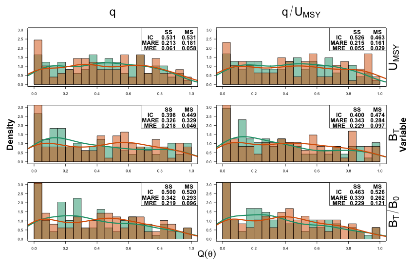
Finally, for each parameter we calculated the distribution of predictive quantiles over replicates , defined as
where is the normal probability density function with mean and standard deviation . The resulting distribution of quantiles is best interpreted graphically, and indicates how well the model is estimating parameter uncertainty. Well performing estimators will have a near-uniform distribution of values, because true values should be distributed randomly across the full domain of the parameter’s sampling distribution. Estimators that under-represent uncertainty by produce standard errors that are too small and will, therefore, have excess density near and (i.e a -shaped graphical distribution), indicating that true values have larger -scores in the sampling distribution. Models that over-represent uncertainty have standard errors that are too large and will collect density near (i.e. a -shaped graphical distribution), indiciating lower -scores of true values in the sampling distribution.
We used an experimental design approach for simulation models to analyse the effects of experimental factors and assessment model configurations on the MARE and performance metrics (Kleijnen 2008). This method attmpts to simplify the complex response surfaces via a generalized linear meta-model of teh response surface to simulation model inputs (i.e. factor levels and assessment model prior configurations)(McCullagh 1984). Meta-models are defined in the supplemental material.
Assessment for British Columbia dover sole
We fit all 8 multi-stock assessment model configurations and the single-stock assessment model to the dover sole data for the three stocks in Figure 2. We initialized all stocks in a fished state, beginning in 1984 for the HS stock, and 2003 for both QCS and WCVI stocks.
For the prior on and , we used a prior mean value of and , keeping the relative standard deviation at 100%. For the process error variances, we tested two hypotheses for the strength of environmental effects on population dynamics. These were implemented as choices for the parameters of the inverse-gamma prior distributions on process error variance terms, when using . The first choice was to use , placing the prior mode at around , favouring process errors with a larger standard deviation around . The second was to use , reducing the prior mode to , favouring process errors with a small standard deviation around .
For each model fit, we calculated Akaike’s information criterion, which we corrected for the sample size (number of years of survey data) for each stock (AICc) (Burnham and Anderson 2003). We then selected the group of multi-stock configurations that performed the best under both hypotheses according to their AICc values, and present estimates of optimal harvest rate , terminal biomass , optimal biomass , relative biomass , and current fishing mortality relative to the optimal harvest rate , as well as standard errors for all estimates. We used the sum of single-stock AICc values to represent the complex aggregate AICc score for comparing single-stock and multi-stock model fits. While this may be a slight deviation in use of the AIC, we believe it is both useful and satisfies the restrictions of the AICc, i.e., the collection of single-stock models is fit to the same data as the multi-stock models, and the process of adding AICc values is analogous to adding single-stock model log-likelihood values within a joint likelihood.
Results
When discussing experimental results, we restrict our attention to stock , a low information stock if in the information scenarios, and identical to the remaining stocks otherwise. We intially focus on the meta-model effects on MARE ratios and complex aggregate to interpret model configuration effects, and use the remaining metrics to help interpret factor effects.
Single-stock versus multi-stock assessments of the base operating model
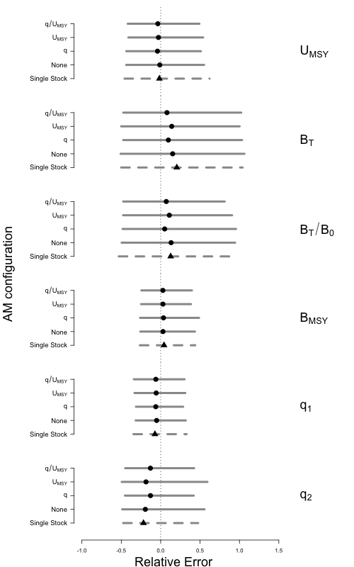
As expected, shrinkage effects from hierarchical multi-stock assessment models often improved precision of key management parameter relative errors from multi-stock models compared to single-stock models, when fit to data from the base operating model (Figure 4). Although this pattern extended across most model configurations and variables, the effect was most noticeable for optimal harvest rate and optimal biomass , and weakest for absolute and relative terminal biomass. Also, the effects of hierarchical priors were most noticeable for parameters that were subject to those priors, i.e. catchability had larger increases in precision under a model configurations that estimated a shared prior on catchability (Figure 4, under the AM configuration).
We found that estimator bias was less sensitive to hierarchical multi-stock configurations, with sometimes very subtle effects. For example, for optimal harvest rate , optimal biomass , and survey 1 catchability estimates were all relatively unbiased under the single-stock model, and all multi-stock model configurations had a negligible effect on the bias (Figure 4). In contrast, survey 2 catchability , and absolute and relative terminal biomass and were biased under the single-stock model, so were themselves very sensitive. As with precision, the bias of catchability was most reduced by the and configurations, and these improvements translated directly into reductions in absolute bias of the terminal biomass estimates and .
The other performance metrics indicated that the and configurations performed similarly under the base operating model. For the management parameters most useful in setting harvest advice, productivity and current biomass , the configuration either improved all metrics, or kept metrics within a tolerable level of the ideal (Figure 5), e.g. interval coverage fell for , but remained within 10% of the nominal level. Similarly, predictive quantile distributions were slightly more uniform under the configuration than the single-stock model, indicating an improvement in estimator precision and bias, however the difference between and configurations was subtle. Plots of the full set of metrics for all multi-stock model configurations and parameters under the base operating model can be found in the supplementary material (Figures S1 - S4).
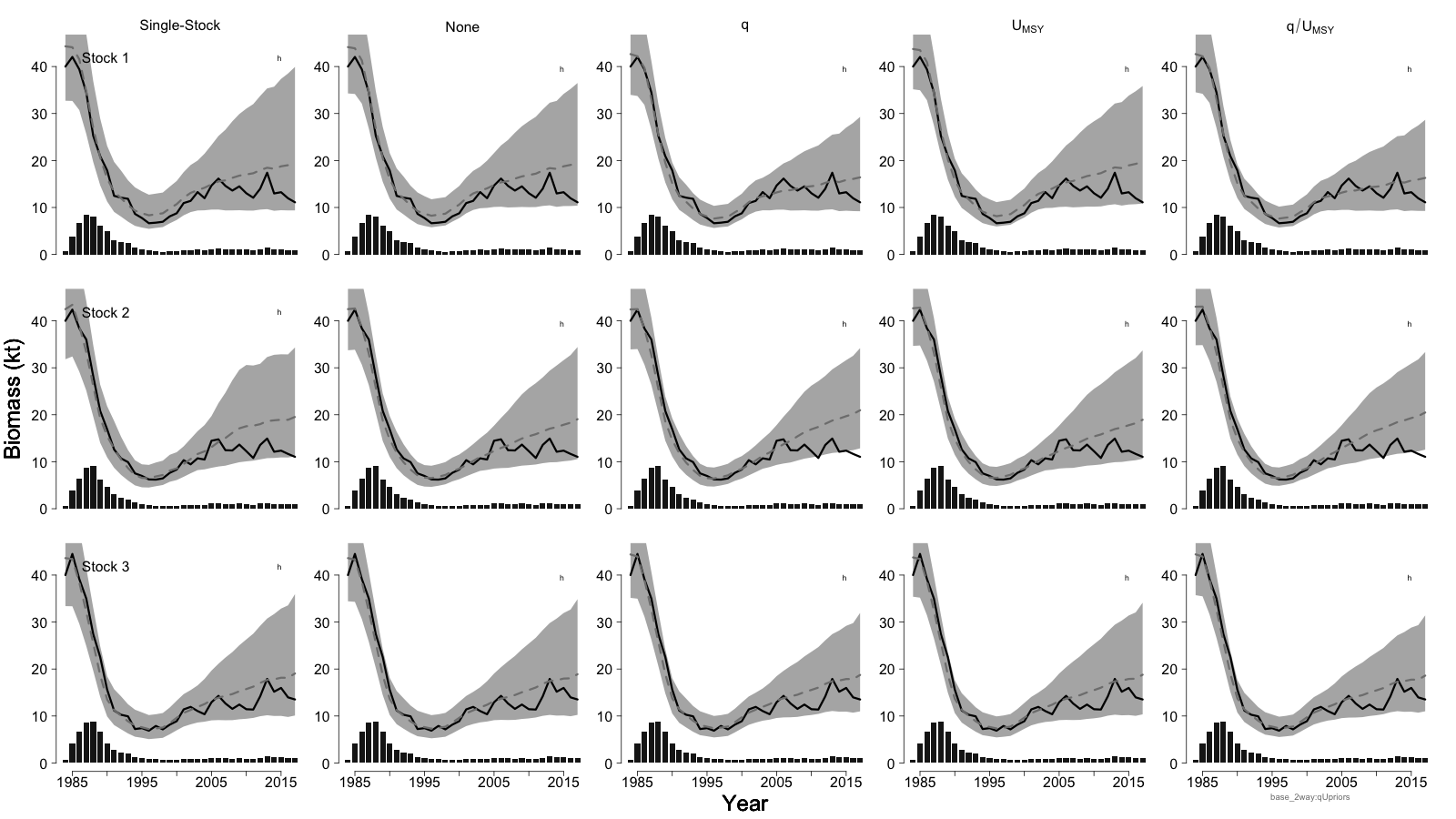
Increased precision in catchability and biomass parameters under hierarchical multi-stock models was not always a benefit. Under a single simulation replicate, 95% confidence intervals of biomass estimates from joint models were generally more precise than single-stock estimates; however, increased precision occasionally created estimates that were overprecise, leaving true biomass values outside confidence intervals (Figure 6, Stock 2, and models). Furthermore, hierarchical estimation appeared to falsely detect an increasing trend in biomass, where the single-stock model was more conservative (Figure 5, Stock 2), but corrected the same behaviour in the single-stock model for a different stock in the same complex (Figure 5, Stock 1).
Simulation Experiment Results
Model configuration effects
When comparing MARE values through the metric, multi-stock model configurations that estimated the shared prior on survey catchability, denoted and , stood out as the most beneficial for parameters of the low data quality stocks (stock ). Both of these configurations increased values, or had effects that were within 1 standard error of zero (Table 4, Stock 1 values), indicating that multi-stock model configurations produced MARE values at most equal to those produced by single-stock models.
As under the base operating model, according to the metric the best performing hierarchical multi-stock model for providing harvest advice was . Closer inspection of and values indicated that estimation of the mean optimal harvest rate reduced the larger benefit to catchability in both surveys and optimal biomass (Table 4, and ). On the other hand, while the prior had not effect on terminal biomass , the effects on relative biomass were nearly tripled over the reference level . The values for optimal biomass and catchability parameters were lower, but these parameters are not particularly critical for providing harvest advice.
The and configurations stood out at the complex level also, with higher meta-model coefficients than the configuration (Table 4, Complex Aggregate Values). Under the aggregate MARE ratio , it was more difficult to separate the two best models as the meta-model coefficients for both and were closer together, e.g. , and there was a reduction in under the configuration. Unlike the stock-specific values, the prior configuration had an effect on the response in the aggregate, where the configuration produced the biggest reduction . On the other hand, the largest increase over the null model reference level was also produced by the configuration for the response, indicating a tradeoff between estimates of stock status and productivity.
The configuration tended to perform the worst according to the metric. We expected to see a benefit to productivity parameter estimates but we were surprised to find there was no benefit to a low data quality stock. Moreover, meta-model coefficients for and response variables were consistently smaller than the other configurations, and often negative or insignificant.
Factor effects
As expected, the effects of shrinkage were most beneficial under low-information scenarios, according to the metrics. When the biomass was initialized in a fished state, and values increased (Table 4, ). Similarly, there were significant increases in and values for all parameters when the assessments were initialized at the beginning of survey 2 (Table 4, ). These improvements under low information conditions are largely driven by a stabilising effect of shrinkage. That is, single-stock models produced relatively larger MARE values as data data quality was reduced. Under the same conditions, the hierarchical multi-stock models were restricted from increasing MARE values as fast by shrinkage (Table 4).
We found that the and configurations were sensitive to data quality and the choice of performance measure. For example, under a 1-way trip fishing history with 4 identical stocks (Figure 7), the configuration eliminatedd bias in and improved interval coverage from 62% to 56%, correcting an under-precise estimator. In contrast, the configuration was over-precise, indicated by an interval coverage of 33% and the quantile distribution becoming slightly -shaped, and also increased bias in estimates (Figure 7, ).
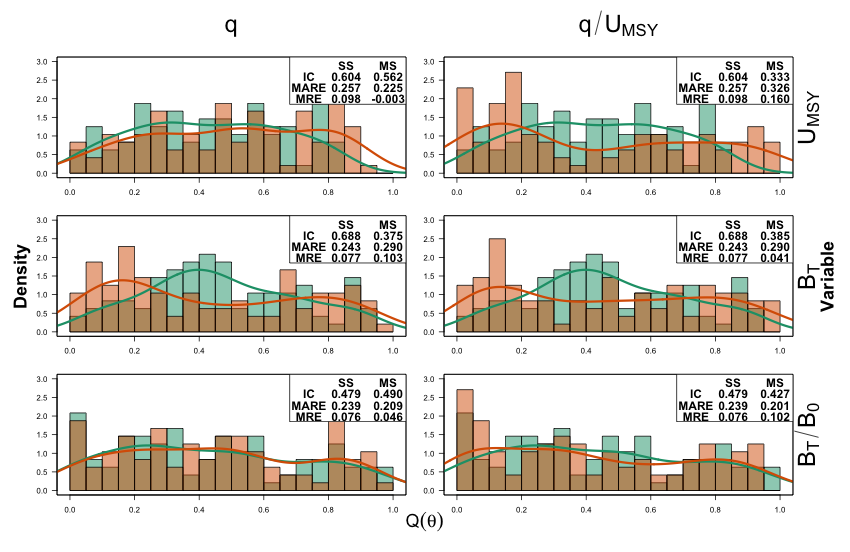
On the other hand, the configuration appeared to perform better under a 2-way trip fishing history, a short time series, and fished initialisation. The configuration reduced bias for relative biomass and almost eliminated bias for (Figure 8, ). Interval coverage also improved under the configuration for terminal biomass estimates and , coming closer to the nominal rate of 50%. Although the interval coverage fell to 36% under the configuration, indicating an over-precise estimator, we viewed this as favourable compared to the configuration, where was under-precise by a similar amount, yet remained positively biased.
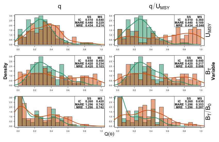
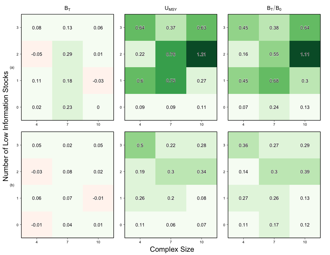
The effect of complex size and the number of low information stocks interacted in unexpected ways. According to the selected meta-model, the size of the complex and the number of low information stocks appeared to have little effect on response values. Indeed, all and effects on and values were at most in magnitude, if they were included at all. These weak effects indicated that the linear meta-model is probably too simple for these factors (Figure 9). Increasing the number of low-information stocks was always an improvement for values when moving from to . This was was expected given that the values were calculated for stock (a data poor stock if ), and we expected that multi-stock models and single-stock models would have similar estimates when fit to complexes of data-rich stocks. Beyond any improvements in MARE values were dependent on the size of the complex. Generally, it appeared that keeping the number of low information stocks under half of the complex size, i.e. , preserved the most benefit in terms of precision, though this pattern reversed for and . Complex aggregate values were comparatively flatter in response to the levels of . We didn’t produce response surfaces for other factor combinations as these factors all had 2 levels each, meaning that a linear model should capture the average behaviour.
Assessments of British Columbia dover sole
Multi-stock models defined by shared catchability and shared catchability and optimal harvest rate configurations performed best for the British Columbia dover sole complex based on AICc values. These same configurations also performed best in in the simulation experiments. The configuration and the null model both had AICc scores more than 500 points higher than the best performing multi-stock configuration. The selected multi-stock models gave AICc scores between 100 and 200 units below the total single-stock model scores under both hypotheses (Table 5, AICc), indicating that the increase in estimated parameters was justified. All models had lower AICc values under the assumption of low process error variance.
Hierarchical multi-stock models reduced parameter uncertainties when compared to single-stock models. Multi-stock models with shared priors produced lower cofficients of variation, defined as , for estimates of optimal biomass and productivity parameters, reducing coefficients of variation below 100% in some cases (single-stock vs multi-stock models in Table 4). Similar reductions in uncertainty are visible in reconstructions of stock biomass time series (Figure 10).
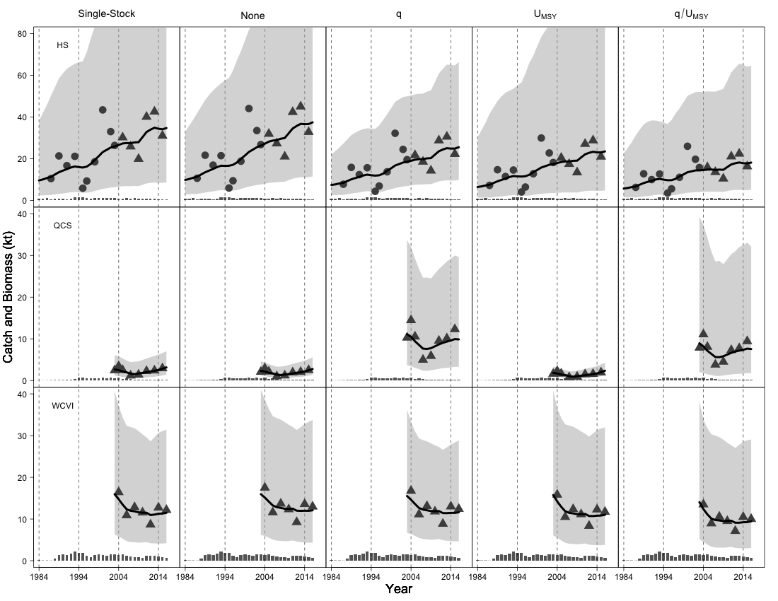
Assessments of the dover sole complex were qualitatively similar between model configurations and hypotheses. The major differences between assessment model configurations were the level of uncertainty in parameter estimates, and the scale of each individual stock’s biomass, but the trends over time were the same (Figure 10). The Hecate Strait (HS) stock showed increasing biomass since 1984, with more or less process variation depending on the configuration and variance hypothesis (Figure S5). The Queen Charlotte Sound stock showed an initial depletion with increased landings between 2003 and 2006, followed by some growth that has continued until present day. Finally, the West Coast of Vancouver Island (WCVI) stock showed a flat biomass trend following initial depletion from 2003 to 2006. The flat trend in the WCVI stock may indicate that fishing was balancing annual production.
We found that the multi-stock assessment model configuration generally estimated all stocks as smaller and more productive than other assessments (Table 5). This was most noticable for the QCS stock biomass estimates by multi-stock models, where the single-stock model considered the optimal biomass to be close to 18 kt, with a terminal relative biomass between 7% and 13%, in contrast to the selected multi-stock configurations, where optimal biomass was between 3 kt and 6 kt, with a current relative biomass between 95% and 110%. Under the single-stock model configuration, the biomass scales corresponded to expected catchability values of , and . We considered this distribution of catchability values between stocks of the same species unlikely, given that the biomass indices are relative biomass values and catchability corresponded to trawl efficiency. It was more likely that the single-stock assessment reduced the biomass parameter estimates for the QCS stock because of the fished initialisation in 2003. Starting in this state removed any depletion signal from the earlier catch history, and allowing the model to explain the stock indices catch with a smaller biomass.
No selected multi-stock model indicated that dover sole stocks were overfished or experiencing overfishing, however, the uncertainty in relative terminal biomass and harvest rate was often very high. That is, current relative biomass estimates were always at least 60% of unfished, but their coefficients of variation were in some cases above 50% of the mean estimate (Table 5). Similarly, although relative harvest rate estimates were all at most 70% of the optimal harvest rate (Table 5), their coefficients of variation were at least 65%, and sometimes greater than 100%, of the mean estimate for each stock under some model configurations, most often under the high variance assumption.
The hierarchical multi-stock model configuration had the best fit to the data, which is not surprising given that the dover sole complex closely matches the scenario shown in Figure 8, with a fished initialisation and 2 stocks having short time-series of observations. Under those simulation experiments, the configuration was considered over-precise, but essentially unbiased, for estimates. In contrast, for assessments of dover sole data with low process error variance, the precision seems be lower under the configuration, indicated by larger coefficients of variation (Table 5).
Discussion
Our simulation results indicate that, as expected, shrinkage effects in hierarchical multi-stock assessment models are most beneficial when some data sets have low statistical power. Furthermore, both configurations that estimated a shared catchability prior performed best for estimating key management parameters. On the other hand, we found that shrinkage does not always improve stock assessment performance relative to a single-stock approach. In particular, the benefits of joint estimation depend on several factors, including the information content of the data, the choices for hierarchical model priors, and the particular management parameters of interest.
Model configurations that shared prior distributions on survey catchability ( and ) stood out as the best options for improving parameter estimates for stocks with low data quality. This result may occur because catchability is a linear parameter within the assessment, while optimal harvest rate parameters are embedded within non-linear popoulation dynamics. Although this hypothesis does not explain how different configurations increase or reduce bias and precision, it may provide a template to guide expectations and generate hypotheses when testing other hierarchical model behaviour.
We found that simply adding a joint likelihood can have positive effects, which was surprising because there should be no mathematical difference between optimising a set of single-stock models independently vs binding them in a joint model by simply adding their negative log likelihoods together. This result may indicate a stabilising effect from the joint likelihood, where simply including data-rich species without shared priors improves the numerical performance of minimisation algorithm.
There was mixed evidence that increasing the size of the assessment complex produced better results under hierarchical multi-stock models. For instance, in the lower information scenarios, the effect of the complex size depended on the number of low-information stocks present in the system. The most benefit for the first stock was realized when moving from no low information stocks () to one low information stock (). This is counter-intuitive, as decreasing information should reduce precision, but represents the stability induced by the shrinkage from the multi-stock models. Looking at response surfaces averaged over all factor levels and configurations, we found that complexes of size provided the most stable benefit (in terms of MARE values) for different numbers of low information stocks ; however, we weren’t testing for an optimal size, which would require a new design with a finer resolution on and factors.
Some of our results may be caused by a discrepancy between the underlying assumption of normality for parameter distributions used in the Laplace approximation to the integrated likelihood and the true parameter distribution (Kristensen et al. 2015). Despite the integrated likelihood, the approximation by a normal distribution means that there is potential for bias caused by disagreement between the modes of the assumed normal distribution and true parameter distribution (Stewart et al. 2013).
Although we investigated a single-species, multi-stock complex, where stocks represented biologically identical management units within the dover sole fishery, the hierarchical multi-stock approach could be extended to a multi-species approach by simulating stocks with different biological parameters and . We suspect that a differences in unfished biomass would not have a strong effect on overall performance. In a Schaefer model context, the unfished biomass parameter determines the absolute scale at which the dynamics operate, but has little effect on the dynamics themselves. Density dependence in annual production is driven by this parameter, but that effect is independent of absolute biomass and relies, instead, on the relative biomass . In contrast, differences among intrinsic growth rates may improve estimates in assessment models that estimate shared productivity priors. More productive stocks would grow faster when fishing pressure is reduced, reducing uncertainty in productivity estimates for those stocks. Stocks with more precise estimates may then have a dominating effect on the hierarchical prior, improving hierarchical assessments but potentially biasing estimates of weaker stock productivities (Raudenbush and Bryk 2002).
Multi-species extensions to the framework we’ve presented here may also provide deeper insights. For example, introducing age-structured population dynamics (Fournier et al. 1998), or a delay-difference formulation (Schnute 1985), would differentiate multiple species further than a simple Schaefer model by allowing for different maturation delays, growth rates, and recruitment dynamics to affect stock production. If biological data were unavailable for informing life-history parameter estimates under more realistic population dynamics, meta-analyses of Beverton-Holt life history invariants within family groups could provide informative prior distributions (Nadon and Ault 2016). Indeed, recent meta-analyses have shown that publically available data-bases of life history parameters can be useful for this type of application (Thorson et al. 2014). Similar meta-analyses of the same data-bases, comparing species that are evolutionarily related, improves the utility of life history invariants by estimating different ratios within taxa, improving their utility as informative priors and potentially providing inverse-gamma priors on hierarchical variance terms in the form of evolutionary covariance estimates (Thorson et al. 2017).
We made several simplifying assumptions about the population dynamics for simplicity in design and interpretation. In addition to assuming that biological parameters are the same for stocks within the complex, we assumed fishing pressure was identical among stocks, and the magnitude of species-specific effects was identical. The choice of identical biology removed a “stock-effect” on management parameter estimates, as discussed above for productivity. With different biological parameters, the ability to identify hierarchical estimator effects may be reduced due to confounding with stock effects. Next, subjecting stocks to identical fishing pressure simplifed the generation of assessment data. Simplifying the simulations in this way may have increased the correlation between stocks, improving performance of the hierarchical multi-stock estimators relative to more realistic situations. For example, it would be more realistic to link fishing mortality to fishing effort through a stock-specific fishery catchability.
We also made simplifying assumptions when defining the assessment model treatment of stock-specific effect . These assumptions were identical standard deviations, which matched the simulated dynamics, zero correlation in process errors, which did not match the simulated dynamics, and we avoided estimating the shared year effect , despite simulating these effects. The reason for the second assumption was for stability in simulation trials, as estimating the correlation often produced nonsensical results. It may be possible to address this by applying an inverse Wishart prior for the full estimated covariance matrix, but we did not consider this within the scope of this research. We avoided estimating the shared year effect as this was removed from the experimental design after it was clear that we would be unable to reliably estimate it, and there was no benefit to partitioning the variance across an extra process error term. Adding another data stream, such as an environmental index (Malick et al. 2015), or forcing the year effects to resemble a periodic or trend-zero behaviour (Walters 1986), may improve these estimates in other studies.
We did not conduct sensitivity analyses of the hyperpriors. Intuitively, we expect that more precise inverse-gamma hyperpriors on estimated variance parameters would increase the shrinkage effect, and thereby clustering stock-specific estimates closer to a biased mean value. Instead of focusing on the behaviour induced by hyperprior settings, we chose instead to focus on the behaviour induced by defining the shared priors, and left the hyperpriors on prior means sufficiently vague to emulate the true prior knowledge about the dover sole complex, and on prior variances sufficiently informative to encourage a shrinkage effect.
Fitting the hierarchical multi-stock surplus production models assessment to dover sole data showed that shrinkage effects carried over to a real system. Shrinkage effects reduced uncertainty when data had low statistical power, and provided more realistic estimates of catchability parameters than single-stock models, especially for the Queen Charlotte Sound stock. While the resulting estimates were sometimes quite uncertain, and a full assessment would require more scrutiny or a different model structure than we have provided here, our results indicate that all three dover sole stocks are likely in a healthy state given recent rates of exploitation.
Conclusion
Our results confirm that hierarchical multi-stock production models are a feasible data-limited approach to stock assessment in multi-stock fisheries. Under low statistical power conditions, hierarchical multi-stock assessment modeling is preferable to data-pooling approaches for at least two reasons. First, hierarchical multi-stock models are able to produce stock-specific estimates that allow management decisions to be made at a higher spatial resolution and based on data rather than strong a priori assumptions or management parameter values averaged over stocks. Despite the potential for bias under low-power conditions, stock-specific estimates of key management parameters can provide meaningful and important feedback in the fishery management system. Second, using a hierarchical multi-stock method ensures that an assessment framework is readily available for more and better data, making it much easier to update model estimates later when more data is available. Moreover, they type of additional data to be collected could be prioritized by examining the standard errors for observation model components of the hierarchical multi-stock assessment models, where higher uncertainty may indicate a better return on investments in improved monitoring.
The feasibility of hierarchical multi-stock surplus production models relies on catch and effort data being available, but we consider hierarchical multi-stock production models as an important bridge between catch-only methods and more data-intensive methods. For instance, some catch only methods require restrictive a priori assumptions, such as an estimate of relative biomass as a model input (MacCall 2009, Dick and MacCall 2011). More recently, a multi-species assessment method was derived that removes the need for relative biomass estimates, but requires restrictive assumptions about fishery-dependent catchability and that all species are initially in an unfished state (Carruthers 2018). Our approach avoids all of these assumptions. For instance, (i) joint model estimates of relative biomass were stable in practice, and in simulations despite absence of a current relative biomass estimate (or assumption); (ii) hierarchical multi-stock models have better precision when initialized in fished states; and (iii) fishery catchability assumptions are not required. Thus, while the data needs are higher for our approach, the potential applications are broader in scope.
On the other hand, hierarchical multi-stock models should be scrutinized closely via standard assessment performance measures (e.g., retrospective analysis) before application to real management systems. In particular, we found that shrinkage can have unexpected non-linear side-effects. Closed-loop simulations would be needed to determine the long-term implications of these types of errors on multi-stock harvest management systems (Punt et al. 2016).
Acknowledgements
Our funding for this research was provided by a Mitacs Cluster Grant to S. P. Cox in collaboration with Wild Canadian Sablefish, the Pacific Halibut Management Association and the Canadian Groundfish Research and Conservation Society. We specifically thank A. R. Kronlund and M. Surry at the Fisheries and Oceans Pacific Biological Station for fulfilling data requests and helpful comments on earlier versions of the manuscript. Further support to S.P.C. and S.D.N.J. were provided by an NSERC Discovery Grant to S. P. Cox. We’d also like to thank the associate editor and one anonymous reviewer for helpful comments during the peer review of this manuscript.
References
Arreguı’n-Sánchez, F. 1996. Catchability: A key parameter for fish stock assessment. Reviews in fish biology and fisheries 6(2): 221–242. Springer.
Burnham, K.P., and Anderson, D.R. 2003. Model selection and multimodel inference: A practical information-theoretic approach. Springer Science & Business Media.
Carlin, B.P., and Louis, T.A. 1997. Bayes and empirical bayes methods for data analysis. In Statistics and Computing. Springer.
Carruthers, T.R. 2018. A multispecies catch-ratio estimator of relative stock depletion. Fisheries Research 197: 25–33. Elsevier.
Carruthers, T.R., Punt, A.E., Walters, C.J., MacCall, A., McAllister, M.K., Dick, E.J., and Cope, J. 2014. Evaluating methods for setting catch limits in data-limited fisheries. Fisheries Research 153(0): 48–68. doi: http://dx.doi.org/10.1016/j.fishres.2013.12.014.
Cox, S., Kronlund, A., and Lacko, L. 2011. Management procedures for the multi-gear sablefish (anoplopoma fimbria) fishery in british columbia, canada. Can. Sci. Advis. Secret. Res. Doc 62.
Dick, E., and MacCall, A.D. 2011. Depletion-based stock reduction analysis: A catch-based method for determining sustainable yields for data-poor fish stocks. Fisheries Research 110(2): 331–341. Elsevier.
Fargo, J. 1998. Flatfish stock assessments for the west coast of Canada for 1997 and recommended yield options for 1998. Canadian Stock Assessment Secretariat Research Document.
Fargo, J. 1999. Flatfish stock assessments for the west coast of Canada for 1999 and recommended yield options for 2000. DFO Can. Stock. Assess. Sec. Res. Doc. (1999/199): 51.
Fournier, D.A., Hampton, J., and Sibert, J.R. 1998. MULTIFAN-cl: A length-based, age-structured model for fisheries stock assessment, with application to south pacific albacore, thunnus alalunga. Canadian Journal of Fisheries and Aquatic Sciences 55(9): 2105–2116. NRC Research Press.
Gelman, A., Carlin, J.B., Stern, H.S., and Rubin, D.B. 2014. Bayesian data analysis. Taylor & Francis.
Hilborn, R. 1979. Comparison of fisheries control systems that utilize catch and effort data. Journal of the Fisheries Board of Canada 36(12): 1477–1489. NRC Research Press.
Hilborn, R., and Walters, C.J. 1992. Quantitative fisheries stock assessment: Choice, dynamics and uncertainty/book and disk. Springer Science & Business Media.
James, W., and Stein, C. 1961. Estimation with quadratic loss. In Proceedings of the fourth berkeley symposium on mathematical statistics and probability. pp. 361–379.
Jiao, Y., Cortés, E., Andrews, K., and Guo, F. 2011. Poor-data and data-poor species stock assessment using a bayesian hierarchical approach. Ecological Applications 21(7): 2691–2708. Wiley Online Library.
Jiao, Y., Hayes, C., and Cortés, E. 2009. Hierarchical Bayesian approach for population dynamics modelling of fish complexes without species-specific data. ICES Journal of Marine Science: Journal du Conseil 66(2): 367–377. Oxford University Press.
Kleijnen, J.P. 2008. Design and analysis of simulation experiments. Springer.
Kristensen, K., Nielsen, A., Berg, C.W., Skaug, H., and Bell, B. 2015. TMB: Automatic differentiation and laplace approximation. arXiv preprint arXiv:1509.00660.
MacCall, A.D. 2009. Depletion-corrected average catch: A simple formula for estimating sustainable yields in data-poor situations. ICES Journal of Marine Science: Journal du Conseil 66(10): 2267–2271. Oxford University Press.
Magnusson, A., and Hilborn, R. 2007. What makes fisheries data informative? Fish and Fisheries 8(4): 337–358. Wiley Online Library.
Malick, M.J., Cox, S.P., Peterman, R.M., Wainwright, T.C., Peterson, W.T., and Krkošek, M. 2015. Accounting for multiple pathways in the connections among climate variability, ocean processes, and coho salmon recruitment in the northern california current. Canadian Journal of Fisheries and Aquatic Sciences 72(10): 1552–1564. NRC Research Press.
McCullagh, P. 1984. Generalized linear models. European Journal of Operational Research 16(3): 285–292. Elsevier.
Mueter, F.J., Ware, D.M., and Peterman, R.M. 2002. Spatial correlation patterns in coastal environmental variables and survival rates of salmon in the north-east pacific ocean. Fisheries Oceanography 11(4): 205–218. Wiley Online Library.
Nadon, M.O., and Ault, J.S. 2016. A stepwise stochastic simulation approach to estimate life history parameters for data-poor fisheries. Canadian Journal of Fisheries and Aquatic Sciences 73(12): 1874–1884. NRC Research Press.
Peterman, R.M. 1990. Statistical power analysis can improve fisheries research and management. Canadian Journal of Fisheries and Aquatic Sciences 47(1): 2–15. NRC Research Press.
Peterman, R.M., Pyper, B.J., Lapointe, M.F., Adkison, M.D., and Walters, C.J. 1998. Patterns of covariation in survival rates of british columbian and alaskan sockeye salmon (oncorhynchus nerka) stocks. Canadian Journal of Fisheries and Aquatic Sciences 55(11): 2503–2517. NRC Research Press.
Punt, A.E. 2003. Extending production models to include process error in the population dynamics. Canadian Journal of Fisheries and Aquatic Sciences 60(10): 1217–1228. NRC Research Press.
Punt, A.E., Butterworth, D.S., Moor, C.L., De Oliveira, J.A., and Haddon, M. 2016. Management strategy evaluation: Best practices. Fish and Fisheries. Wiley Online Library.
Punt, A.E., Smith, A.D., and Cui, G. 2002. Evaluation of management tools for australia’s south east fishery. 1. Modelling the south east fishery taking account of technical interactions. Marine and Freshwater Research 53(3): 615–629. CSIRO.
Punt, A.E., Smith, D.C., and Koopman, M.T. 2005. Using information for data-rich species to inform assessments of data-poor species through bayesian stock assessment methods. Primary Industries Research Victoria.
Punt, A.E., Smith, D.C., and Smith, A.D. 2011. Among-stock comparisons for improving stock assessments of data-poor stocks: The “Robin Hood” approach. ICES Journal of Marine Science: Journal du Conseil 68(5): 972–981. Oxford University Press.
Raudenbush, S.W., and Bryk, A.S. 2002. Hierarchical linear models: Applications and data analysis methods. Sage.
R Core Team. 2015. R: A language and environment for statistical computing. R Foundation for Statistical Computing, Vienna, Austria. Available from http://www.R-project.org/.
Schnute, J. 1985. A general theory for analysis of catch and effort data. Canadian Journal of Fisheries and Aquatic Sciences 42(3): 414–429. NRC Research Press.
Schnute, J.T., and Richards, L.J. 1995. The influence of error on population estimates from catch-age models. Canadian Journal of Fisheries and Aquatic Sciences 52(10): 2063–2077. NRC Research Press.
Stewart, I.J., Hicks, A.C., Taylor, I.G., Thorson, J.T., Wetzel, C., and Kupschus, S. 2013. A comparison of stock assessment uncertainty estimates using maximum likelihood and bayesian methods implemented with the same model framework. Fisheries Research 142: 37–46. Elsevier.
Thorson, J.T., Cope, J.M., Kleisner, K.M., Samhouri, J.F., Shelton, A.O., and Ward, E.J. 2015. Giants’ shoulders 15 years later: Lessons, challenges and guidelines in fisheries meta-analysis. Fish and Fisheries 16(2): 342–361. Wiley Online Library.
Thorson, J.T., Cope, J.M., and Patrick, W.S. 2014. Assessing the quality of life history information in publicly available databases. Ecological Applications 24(1): 217–226. Wiley Online Library.
Thorson, J.T., Munch, S.B., Cope, J.M., and Gao, J. 2017. Predicting life history parameters for all fishes worldwide. Ecological Applications 27(8): 2262–2276. Wiley Online Library.
Walters, C. 1986. Adaptive management of renewable resources. MacMillan Pub. Co., New York, NY.
Tables
| Description | Symbol | Value |
| Unfished Biomass | 40kt | |
| Intrinsic Rate of Growth | 0.16 | |
| Shared Process Error SD | 0.071 | |
| Stock-specific Process Error SD | 0.071 | |
| Simulation Historical Period |
| Description | Levels | Notes |
| Fishing History | 1-way, 2-way trips | Low/High contrast in biomass |
| Complex Size, | 4,7,10 | |
| Low data quality stocks, | 0,1,2,3 | |
| Initial Assessment Year 1984, 2003 | Short or long series of observations ( or of years) | |
| Initial Relative Depletion | 0.4, 0.7, 1.0 | Fished or unfished initialisation |
| No. | Distribution |
| Survey Catchability | |
| Multi-level prior | |
| q.1 | |
| q.2 | |
| q.3 | |
| Single level prior | |
| q.4 | |
| Optimal Harvest Rate | |
| Multi-level prior | |
| U.1 | |
| U.2 | |
| U.3 | |
| Single level prior | |
| U.4 | |
| Prior Configuration | Experimental Factor | ||||||||
| Response | Ref Level | Init. Dep | Init. Assessment | Low Data Stocks | Complex Size | Fishing History | |||
| Low Data Quality Stock () Values | |||||||||
| 0.60 (0.07) | 0.25 (0.09) | 0.04 (0.09) | 0.09 (0.09) | -0.14 (0.04) | 0.35 (0.04) | - | - | - | |
| -0.01 (0.04) | 0.28 (0.05) | -0.02 (0.05) | 0.28 (0.05) | -0.04 (0.02) | 0.08 (0.02) | - | - | 0.11 (0.02) | |
| 0.16 (0.03) | 0.10 (0.04) | -0.07 (0.04) | 0.02 (0.04) | -0.06 (0.02) | 0.11 (0.02) | 0.06 (0.02) | - | -0.02 (0.01) | |
| 0.32 (0.07) | 0.29 (0.10) | 0.13 (0.10) | 0.63 (0.10) | -0.09 (0.04) | 0.30 (0.04) | - | 0.09 (0.04) | 0.14 (0.03) | |
| 0.06 (0.05) | 0.46 (0.07) | -0.01 (0.07) | 0.27 (0.07) | - | 0.15 (0.03) | - | - | 0.06 (0.03) | |
| -0.02 (0.02) | 0.23 (0.03) | -0.05 (0.03) | 0.10 (0.03) | - | - | 0.03 (0.02) | -0.04 (0.01) | 0.08 (0.01) | |
| Complex Aggregate Values | |||||||||
| 0.47 (0.04) | 0.13 (0.04) | -0.07 (0.04) | -0.07 (0.04) | -0.10 (0.03) | 0.21 (0.03) | 0.04 (0.03) | - | -0.03 (0.02) | |
| 0.04 (0.02) | 0.22 (0.02) | -0.03 (0.02) | 0.21 (0.02) | -0.05 (0.01) | 0.11 (0.01) | -0.03 (0.01) | 0.02 (0.01) | 0.07 (0.01) | |
| 0.11 (0.02) | 0.11 (0.02) | -0.05 (0.02) | 0.01 (0.02) | -0.07 (0.01) | 0.09 (0.02) | - | - | 0.03 (0.01) | |
| 0.31 (0.04) | 0.25 (0.04) | 0.03 (0.04) | 0.39 (0.04) | -0.08 (0.02) | 0.24 (0.03) | - | - | 0.06 (0.01) | |
| 0.08 (0.03) | 0.31 (0.03) | -0.02 (0.03) | 0.21 (0.03) | -0.05 (0.02) | 0.15 (0.02) | - | - | 0.08 (0.01) | |
| -0.06 (0.02) | 0.26 (0.02) | -0.04 (0.02) | 0.15 (0.02) | -0.03 (0.01) | - | - | -0.02 (0.01) | 0.07 (0.01) | |
| Single-Stock Assessment MARE values | |||||||||
| 40.52 (1.22) | - | - | - | -6.64 (1.49) | 4.44 (1.21) | 3.90 (1.66) | - | -9.00 (1.08) | |
| 29.01 (0.56) | - | - | - | -0.96 (0.64) | 2.62 (0.54) | - | 1.01 (0.62) | 2.65 (0.51) | |
| 26.61 (0.49) | - | - | - | -5.56 (0.60) | 3.67 (0.49) | 3.11 (0.67) | -0.77 (0.54) | - | |
| 56.13 (1.97) | - | - | - | -11.68 (2.28) | 17.71 (1.93) | - | - | 14.34 (1.81) | |
| 19.58 (0.44) | - | - | - | - | 3.46 (0.44) | - | - | - | |
| 17.97 (0.41) | - | - | - | - | 0.59 (0.41) | - | -0.94 (0.49) | -1.00 (0.40) | |
| Multi-Stock Assessment MARE values | |||||||||
| 24.96 (0.87) | -3.54 (1.20) | 0.55 (1.20) | -0.13 (1.20) | -1.70 (0.59) | -0.88 (0.47) | 1.13 (0.65) | -0.78 (0.52) | -5.14 (0.42) | |
| 29.10 (0.76) | -6.22 (1.06) | 0.67 (1.06) | -5.80 (1.06) | - | 0.64 (0.39) | - | 0.76 (0.46) | - | |
| 22.85 (0.78) | -1.85 (1.06) | 1.28 (1.06) | -0.32 (1.06) | -4.23 (0.52) | 1.28 (0.42) | 1.90 (0.58) | - | - | |
| 40.65 (1.87) | -8.77 (2.56) | -5.02 (2.56) | -13.88 (2.56) | -5.47 (1.26) | 4.24 (1.02) | 2.49 (1.40) | -1.67 (1.12) | 6.22 (0.91) | |
| 18.51 (0.75) | -5.39 (1.04) | -0.06 (1.04) | -3.33 (1.04) | 0.69 (0.46) | 1.64 (0.39) | - | - | -1.37 (0.37) | |
| 18.51 (0.81) | -3.73 (1.15) | 1.24 (1.15) | -1.54 (1.15) | - | - | - | - | -2.58 (0.41) | |
| High Process Error Variance | Low Process Error Variance | ||||||||
| Model Config | HS | QCS | WCVI | Total | Model Config | HS | QCS | WCVI | Total |
| Single-Stock | 0.147 (0.69) | 0.066 (1.14) | 0.122 (0.94) | - | Single-Stock | 0.113 (0.77) | 0.100 (0.71) | 0.136 (0.84) | - |
| 0.127 (0.64) | 0.092 (0.88) | 0.095 (0.90) | - | 0.115 (0.63) | 0.097 (0.83) | 0.104 (0.83) | - | ||
| 0.205 (0.64) | 0.191 (0.73) | 0.214 (0.78) | - | 0.156 (0.76) | 0.151 (0.74) | 0.170 (0.86) | - | ||
| Single-Stock | 33.189 (1.04) | 4.841 (1.27) | 11.487 (0.89) | - | Single-Stock | 29.641 (1.13) | 2.868 (0.66) | 10.956 (0.83) | - |
| 27.112 (0.82) | 13.843 (0.85) | 13.616 (0.74) | - | 25.498 (0.79) | 9.873 (0.87) | 11.618 (0.77) | - | ||
| 21.067 (0.91) | 11.246 (0.93) | 11.685 (0.83) | - | 18.124 (0.96) | 7.553 (1.05) | 9.457 (0.88) | - | ||
| Single-Stock | 0.968 (0.67) | 0.131 (1.97) | 0.718 (0.80) | - | Single-Stock | 0.874 (0.48) | 0.077 (1.53) | 0.700 (0.59) | - |
| 0.917 (0.62) | 1.091 (0.73) | 0.702 (0.92) | - | 0.842 (0.47) | 0.950 (0.47) | 0.631 (0.70) | - | ||
| 0.932 (0.57) | 1.071 (0.56) | 0.830 (0.52) | - | 0.878 (0.41) | 0.967 (0.41) | 0.708 (0.54) | - | ||
| Single-Stock | 0.081 (1.03) | 0.597 (1.12) | 0.520 (1.11) | - | Single-Stock | 0.117 (0.83) | 0.669 (0.65) | 0.488 (0.96) | - |
| 0.114 (0.85) | 0.151 (1.07) | 0.560 (1.04) | - | 0.134 (0.67) | 0.199 (1.03) | 0.602 (0.97) | - | ||
| 0.091 (0.87) | 0.089 (1.00) | 0.291 (0.95) | - | 0.139 (0.66) | 0.168 (1.01) | 0.453 (0.88) | - | ||
| Single-Stock | 17.143 (0.90) | 18.415 (1.53) | 8.004 (0.88) | - | Single-Stock | 16.951 (1.11) | 18.672 (1.48) | 7.830 (0.72) | - |
| 14.790 (0.73) | 6.343 (0.91) | 9.693 (0.95) | - | 15.142 (0.80) | 5.196 (0.81) | 9.210 (0.72) | - | ||
| 11.306 (0.83) | 5.250 (0.86) | 7.043 (0.75) | - | 10.323 (0.94) | 3.904 (0.97) | 6.680 (0.78) | - | ||
| Single-Stock | -102.06 | -22.487 | -23.655 | -148.202 | Single-Stock | -163.261 | -54.035 | -56.802 | -274.098 |
| -169.838 | -343.312 | ||||||||
| -252.292 | -417.676 | ||||||||
Figures
Supplementary Material
Experimental Design
Latin Hyper-rectangle Designs
To sample our experimental design space we used a space filling design that we call the latin hyper-rectangle design (LHrD). The LHrD is a modification of the latin hypercube design (LHD), which is a multi-dimensional stratified random sampling approach (Kleijnen 2008). There are a few differences between a classical LHD and our LHrD, but the principle remains the same: LHrDs are a space filling design that test every factor level while avoiding a full factorial design, reducing computational overhead. This reduction in overhead is useful given that multi-stock models are subject to the curse of dimensionality.
The main difference between a LHrD and a LHD is in how the design space is sampled. In LHDs, the dimensions of the design space (the simulation model inputs, or experimental factors) are split into an equal number of segments - thus, a hypercube - and factor levels are sampled from within each segment so that the resulting design has the latin property. In a LHrD, the constraint that each dimension has an equal number of segments is relaxed, forming a hyper-rectangle instead. Again, segments of each dimension are sampled so that the resulting design has the latin property.
There are some features of latin hyper-cubes that are lost when relaxing the equal segments constraint to create latin hyper-rectangles. For example, the dimensions that are broken into more segments have fewer samples, due to the lower number of segments on the “shorter” dimensions of the hyper-rectangle. This is not a huge problem, however, since given sufficiently many dimensions those segments will be sampled in another slice of the hyper-rectangle. In this way, every factor level is tested in combination with multiple levels of other factors, creating a space filling design. We also restricted our design to a so-called deterministic LHrD, where the sampled elements within each segment were the same for every treatment, instead of randomly sampled from within that segment.
We found that defining our own approach that relaxed the hyper-cube constraint was preferable for two main reasons. First, it’s not always necessary to test an equal number of levels for every factor. For example, understanding the effects of one-way and two-way trips probably only requires 2 levels of fishing intensity, whereas using a hypercube design would have required us to arbitrarily define multiple extra scenarios in between the extremes we’ve given in this paper. Second, we considered the time spent on creating this process to be an investment in a method that could be used in future simulation experiments as part of our own work, and potentially the work of others.
Our process for defining a LHrD starts by systematically defining a latin hyper-rectangle with the same number of dimensions as we have factors. Each dimension of the hyper-rectangle is has a number of entries equal to the number of levels for the corresponding factor, and in this way the hyper-rectangle spans the experimental tableau. Sampling the experimental tableau then reduces to sampling the entries of the hyper-rectangle. We followed the steps below to create our design in the R statistical programming language (available at https://github.com/samueldnj/LHrD):
-
1.
Define experimental factors and choose factor levels. The number of factors is the number of dimensions of the hyper-rectangle.
-
2.
Choose the factor with the highest number of levels. This is number of distinct values of hyper-rectangle entries.
-
3.
Create an -dimensional array , and assign each dimension of to correspond to a different experimental factor by setting array dimensions to the number of levels of that factor.
-
4.
Populate the entries of with the integers by adding the dimension indices modulo . For example, if and , the entry in the position of will be , and the entry in the position of will be , etc.
-
5.
In sequence, permute dimensional slices of by applying a random permutation to each dimension’s indices. In R code, for the first dimension: A[1:d_1,,,,] <- A[sample(d_1,d_1),,,,].
-
6.
To choose a sample of experimental treatments, randomly sample . The array indices of each instance of in then correspond to levels of each factor, creating an experimental treatment.
After step 4, the array is a hyper-rectangular array with entries with the latin property. We do not prove this property here, but the key is in the choice of the maximum dimension of the array to be the modulus of entries. Experimental designs can be formed directly from this point using step 6, however in the experimental design literature these designs are considered to be sub-optimal [Kleijnen (2008); Ch 5], as they favour diagonals of the experimental tableau and may then cause dependence between treatments. This is why we apply step 5, where we reduce dependence by randomising entries with permutations, which preserve the latin property. In order to maximise the randomisation of entries, we suggest using randomly selected derangements (permutations that fix no points), however this would require some extra machinery to produce (Martı’nez et al. 2008).
We relied heavily on the established properties of LHDs when developing the LHrD, and as such have not conducted extensive tests on the robustness of this approach. For example, classic LHDs have been refined into “maximin” and “nearly-orthogonal” LHDs, which reduce some of the interdependence between factor levels; however, we did not do this here and leave it for future work or other analysts. Moreover, we did not conduct meta-model validation in our experiments, except for an informal ad-hoc validation when experiments were run multiple times. Each new run produced new random samples of treatments, and the resulting meta-models were often compared. A formal approach to meta-model validation could be easily facilitated using the LHrD framework: simply choose two entries, , and run both designs. A meta-model fit to the results of the design based on could then be validated on the results of design based on , or vice versa.
Our Experimental Design
We give the table for our experimental design below. We added convergence metrics to the table for each scenario and AM configuration, which describe how many attempts were made for each replicate, and how many replicates in total were required to reach 100 converged replicates in each combination.
| Experimental Factor Levels | Prior Configuration | |||||||
| Uhist | initYear | nS | initDep | nDiff | noJointPriors | qPriorOnly | UmsyPriorOnly | qUpriors |
| c(0.2,4,1) | 1984 | 4 | 0.4 | 0 | 100 | 100 | 100 | 100 |
| c(1,1,1) | 2003 | 7 | 0.4 | 0 | 102 | 102 | 102 | 102 |
| c(1,1,1) | 1984 | 10 | 0.4 | 0 | 102 | 101 | 101 | 101 |
| c(0.2,4,1) | 2003 | 10 | 0.4 | 0 | 100 | 100 | 100 | 100 |
| c(1,1,1) | 1984 | 4 | 0.7 | 0 | 104 | 103 | 103 | 102 |
| c(0.2,4,1) | 2003 | 4 | 0.7 | 0 | 100 | 100 | 100 | 100 |
| c(1,1,1) | 2003 | 10 | 0.7 | 0 | 102 | 101 | 101 | 101 |
| c(1,1,1) | 2003 | 4 | 1.0 | 0 | 104 | 103 | 103 | 103 |
| c(0.2,4,1) | 1984 | 7 | 1.0 | 0 | 100 | 100 | 100 | 100 |
| c(1,1,1) | 2003 | 4 | 0.4 | 1 | 104 | 103 | 102 | 102 |
| c(0.2,4,1) | 1984 | 7 | 0.4 | 1 | 100 | 100 | 100 | 100 |
| c(1,1,1) | 1984 | 7 | 0.7 | 1 | 104 | 102 | 101 | 102 |
| c(0.2,4,1) | 2003 | 7 | 0.7 | 1 | 100 | 100 | 100 | 100 |
| c(0.2,4,1) | 1984 | 10 | 0.7 | 1 | 100 | 100 | 100 | 100 |
| c(0.2,4,1) | 1984 | 4 | 1.0 | 1 | 100 | 100 | 100 | 100 |
| c(1,1,1) | 2003 | 7 | 1.0 | 1 | 104 | 102 | 102 | 102 |
| c(1,1,1) | 1984 | 10 | 1.0 | 1 | 103 | 101 | 101 | 101 |
| c(0.2,4,1) | 2003 | 10 | 1.0 | 1 | 100 | 100 | 100 | 100 |
| c(1,1,1) | 1984 | 4 | 0.4 | 2 | 102 | 101 | 102 | 102 |
| c(0.2,4,1) | 2003 | 4 | 0.4 | 2 | 101 | 100 | 100 | 100 |
| c(1,1,1) | 2003 | 10 | 0.4 | 2 | 103 | 101 | 101 | 101 |
| c(1,1,1) | 2003 | 4 | 0.7 | 2 | 102 | 102 | 101 | 102 |
| c(0.2,4,1) | 1984 | 7 | 0.7 | 2 | 100 | 100 | 100 | 100 |
| c(1,1,1) | 1984 | 7 | 1.0 | 2 | 102 | 102 | 102 | 101 |
| c(0.2,4,1) | 2003 | 7 | 1.0 | 2 | 100 | 101 | 100 | 100 |
| c(0.2,4,1) | 1984 | 10 | 1.0 | 2 | 100 | 100 | 100 | 100 |
| c(1,1,1) | 1984 | 7 | 0.4 | 3 | 102 | 101 | 101 | 101 |
| c(0.2,4,1) | 2003 | 7 | 0.4 | 3 | 100 | 101 | 100 | 100 |
| c(0.2,4,1) | 1984 | 10 | 0.4 | 3 | 100 | 100 | 100 | 100 |
| c(0.2,4,1) | 1984 | 4 | 0.7 | 3 | 100 | 100 | 100 | 100 |
| c(1,1,1) | 2003 | 7 | 0.7 | 3 | 102 | 101 | 101 | 101 |
| c(1,1,1) | 1984 | 10 | 0.7 | 3 | 103 | 101 | 101 | 101 |
| c(0.2,4,1) | 2003 | 10 | 0.7 | 3 | 100 | 100 | 100 | 100 |
| c(1,1,1) | 1984 | 4 | 1.0 | 3 | 104 | 103 | 102 | 102 |
| c(0.2,4,1) | 2003 | 4 | 1.0 | 3 | 100 | 100 | 100 | 100 |
| c(1,1,1) | 2003 | 10 | 1.0 | 3 | 102 | 101 | 101 | 101 |
Meta-models for performance metrics
Performance metrics were modeled as responses to experimental factors and assessment model prior configurations using generalised linear “meta-models”. Meta-modeling is a part of a formal approach to simulation experimentation, where outputs of a complex simulation model are viewed as responses to simpler functions of simulation model inputs (Kleijnen 2008). The parameters of the simpler function, or meta-model, are then used to improve interpretation of the results of complex simulation experiments. We used generalised linear meta-models as they are robust to heterogeneous variance of response variable residuals (McCullagh 1984), which were common in our experimental treatment outputs.
For performance metrics we estimated the coefficients of a generalised linear model
for each experiment, where the is the intercept, is the effect of the multi-stock assessment model prior configuration, and the coefficients are the factor effects for factor levels . Numerical explanatory variables, such as the year of initialisation and initial depletion, were scaled to to allow direct comparison of numeric effects with qualitative factor effects. To reduce the number of experimental treatments, we sampled factor levels using a space filling design (Kleijnen 2008). To reduce qualitative factors, we fit the historical fishing intensity and initial year of assessment as continuous variables even though they may not have continuous, or even approximately linear responses. Our reasoning for this is that both factors have 2 levels, and so a linear effect will capture the difference between the level effects sufficiently. For the historical fishing intensity, we regressed on the highest multiple of in the history, that is, for one-way trips, and for two way trips.
In our experiment, the intercept term represents the average response value at the reference levels of qualitative factors in the model. The only qualitative factor we use is the choice of multi-stock model configuration, so the intercept of the models is , representing the “null” multi-stock assessment configuration. When there are no qualitative factors in the meta-model, such as in the models, is simply the average response value over all factors.
Assessment Model Structure
In what follows, we denote by the estimate of a derived or leading model parameter .
Biomass dynamics
We minimized the effect of assessment model mis-specification by matching the deterministic components of the biomass dynamics in the assessment models and the operating model (Eq. 1). In all assessment model configurations the leading biological parameters were and . Biomass time series in the assessment models were initialized at time , either at unfished levels , or at a separately estimated non-equilibrium value when or the initial simulated biomass was below unfished levels. Biomass parameters were penalized by normal prior distributions centered at or near their corresponding true values, i.e.,
which allows estimates to vary within a realistic range by giving each prior a relative standard deviation of 100%.
Productivity prior
When we jointly modeled stock-specific optimal harvest rates , we assumed values shared a log-normal distribution with estimated hyperparameters (U.1, Table 3). The estimated prior mean followed a normal hyperprior (U.2, Table 3) where was randomly drawn from a log normal distribution with a mean of and a standard deviation corresponding to a 20% coefficient of variation. The hyperprior standard deviation was chosen to give a roughly 100% CV in the hyperprior for the prior mean and allow the stock-specific values affect the estimate of more than the hyperprior. We chose a normal prior as this is the least informative while remaining continuous across the whole domain of the parameter space.
The estimated prior variance followed an inverse gamma distribution (U.3, Table 3) with and , to induce a log-normal coefficient of variation of 20% in the shared prior. We chose this prior structure recognizing the shared biology of dover sole stocks implies productivities of similar magnitude (Myers et al. 1999). When we modeled the optimal harvest rates separately we assumed optimal harvest rate parameters followed the hyperprior directly (U.4, Table 3) with the same and values.
Observation models
Similar to the biomass dynamics, we matched the observational model structures for the operating and assessment models (Equation 3). A shared species-level prior distribution was defined for stock-specific catchabilities , with between stock variance . Informative priors were also defined for survey observation error variances , with hyperparameters chosen so that the prior modes were equal to the simulated values for each survey.
Catchability
When we estimated the hierarchical prior on catchability parameters, we used the same model structure for the prior as the simulated catchability model for each survey. Estimates of stock-specific catchability were drawn from a shared log-normal distribution with estimated hyperparameters and (q.1, Table 3). The estimated prior mean followed a normal hyperprior where was drawn randomly as with the prior, with an average of (the average of the two surveys) and 20% CV, while for a 100% hyperprior CV (q.2, Table 3), for similar reasoning as the priors.
The prior variance followed an inverse gamma distribution (q.3, Table 3). Inverse gamma hyperparameters and were chosen induce a value that corresponds to a 20% CV, inducing a shrinkage effect. This prior structure reflects an assumption that dover Sole stocks have a similar availability to survey gear based on similar habitat preferences. Like the productivity prior, when catchability was estimated without a shared prior, we bypassed the mid-level prior, penalizing stock-specific catchability using the normal hyperprior with the same and values to signify no change in prior information (q.4, Table 3). We chose a normal hyperprior because it is less informative than a log-normal distribution, and the mean and variance are chosen to produce a relative standard deviation of 100%, allowing and to vary in a realistic range, but informative enough to induce a shrinkage effect.
Observation errors
Observation errors for each survey were assumed to be drawn from a single log-normal distribution across stocks, with estimated log-standard deviation . To improve convergence in repeated simulation trials, we assumed the estimated log-variance followed an inverse gamma prior distribution
| (4) |
Like the process error variance priors, the hyperparameter was chosen to place the mode of the inverse gamma distribution at the simulated values of when .
Extra performance metrics for the base operating model
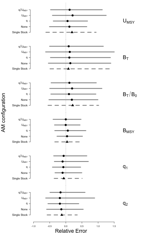
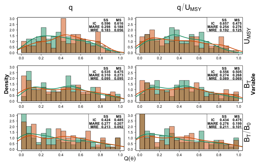
Assessments of British Columbia’s dover sole
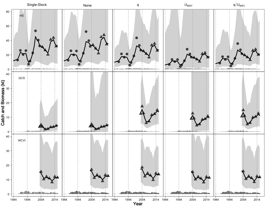
References
Kleijnen, J.P. 2008. Design and analysis of simulation experiments. Springer.
Martı’nez, C., Panholzer, A., and Prodinger, H. 2008. Generating random derangements. In 2008 proceedings of the fifth workshop on analytic algorithmics and combinatorics (analco). SIAM. pp. 234–240.
McCullagh, P. 1984. Generalized linear models. European Journal of Operational Research 16(3): 285–292. Elsevier.
Myers, R.A., Bowen, K.G., and Barrowman, N.J. 1999. Maximum reproductive rate of fish at low population sizes. Canadian Journal of Fisheries and Aquatic Sciences 56(12): 2404–2419. NRC Research Press.