Representation Tradeoffs for Hyperbolic Embeddings

Abstract

Hyperbolic embeddings offer excellent quality with few dimensions when embedding hierarchical data structures like synonym or type hierarchies. Given a tree, we give a combinatorial construction that embeds the tree in hyperbolic space with arbitrarily low distortion without using optimization. On WordNet, our combinatorial embedding obtains a mean-average-precision of $0.989$ with only two dimensions, while Nickel et al.’s recent construction obtains $0.87$ using $200$ dimensions. We provide upper and lower bounds that allow us to characterize the precision-dimensionality tradeoff inherent in any hyperbolic embedding. To embed general metric spaces, we propose a hyperbolic generalization of multidimensional scaling (h-MDS). We show how to perform exact recovery of hyperbolic points from distances, provide a perturbation analysis, and give a recovery result that allows us to reduce dimensionality. The h-MDS approach offers consistently low distortion even with few dimensions across several datasets. Finally, we extract lessons from the algorithms and theory above to design a PyTorch-based implementation that can handle incomplete information and is scalable.

1 Introduction

Recently, hyperbolic embeddings have been proposed as a way to capture hierarchy information for use in link prediction and natural language processing tasks [28, 5]. These approaches are an exciting new way to fuse rich structural information (for example, from knowledge graphs or synonym hierarchies) with the continuous representations favored by modern machine learning.

To understand the intuition behind hyperbolic embeddings’ superior capacity, note that trees can be embedded with arbitrarily low distortion into the Poincaré disk, a model of hyperbolic space with only two dimensions [32]. In contrast, Bourgain’s theorem [27] shows that Euclidean space is unable to obtain comparably low distortion for trees—even using an unbounded number of dimensions. Moreover, hyperbolic space can preserve certain properties; for example, angles between embedded vectors are the same in both Euclidean space and the Poincaré model (the mapping is conformal), which suggests embedded data may be easily able to integrate with downstream tasks.

Many graphs, such as complex networks [24], including the Internet [23] and social networks [36]) are known to have hyperbolic structure and thus befit hyperbolic embeddings. Recent works show that hyperbolic representations are indeed suitable for many hierarchies (e.g, the question answering system HyperQA proposed in [35], vertex classifiers in [5], and link prediction [28]). However, the optimization problem underlying these embeddings is challenging, and we seek to understand the subtle tradeoffs involved.

We begin by considering the situation in which we are given an input graph that is a tree or nearly tree-like, and our goal is to produce a low-dimensional hyperbolic embedding that preserves all distances. This leads to a simple strategy that is combinatorial in that it does not minimize a surrogate loss function using gradient descent. It is both fast (nearly linear time) and has formal quality guarantees. The approach proceeds in two phases: (1) we produce an embedding of a graph into a weighted tree, and (2) we embed that tree into the hyperbolic disk. In particular, we consider an extension of an elegant embedding of trees into the Poincaré disk by Sarkar [32] and recent work on low-distortion graph embeddings into tree metrics [18]. For trees, this approach has nearly perfect quality. On the WordNet hypernym graph reconstruction, this obtains nearly perfect mean average precision (MAP) $0.989$ using just two dimensions, which outperforms the best published numbers in Nickel and Kiela [28] by almost $0.12$ points with $200$ dimensions.

We analyze this construction to extract fundamental tradeoffs. One tradeoff involves the dimension, the properties of the graph, and the number of bits of precision - an important hidden cost. For example, on the WordNet graph, we require almost 500 bits of precision to store values from the combinatorial embedding. We can reduce this number to 32 bits, but at the cost of using 10 dimensions instead of two. We show that for a fixed precision, the dimension required scales linearly with the length of the longest path. On the other hand, the dimension scales logarithmically with the maximum degree of the tree. This suggests that hyperbolic embeddings should have high quality on hierarchies like WordNet but require large dimensions or high precision on graphs with long chains—which is supported by our experiments. A second observation is that in contrast to Euclidean embeddings, hyperbolic embeddings are not scale invariant. This motivates us to add a learnable scale term into a stochastic gradient descent-based Pytorch algorithm described below, and we show that it allows us to empirically improve the quality of embeddings.

To understand how hyperbolic embeddings perform for metrics that are far from tree-like, we consider a more general problem: given a matrix of distances that arise from points that are embeddable in hyperbolic space of dimension $d$ (not necessarily from a graph), find a set of points that produces these distances. In Euclidean space, the problem is known as multidimensional scaling (MDS) which is solvable using PCA. A key step is a transformation that effectively centers the points–without knowledge of their exact coordinates. It is not obvious how to center points in hyperbolic space, which is curved. We show that in hyperbolic space, a centering operation is still possible with respect to a non-standard mean. In turn, this allows us to reduce the hyperbolic MDS problem (h-MDS) to a standard eigenvalue problem, and so it can be solved with scalable power methods. Further, we extend classical perturbation analysis [33, 34]. When applied to distances from real data, h-MDS obtains low distortion on graphs that are far from tree like. However, we observe that these solutions may require high precision, which is not surprising in light of our previous analysis.

Finally, we consider handling increasing amounts of noise in the model, which leads naturally into new SGD-based formulations. In traditional PCA, one may discard eigenvectors that have correspondingly small eigenvalues to cope with noise. In hyperbolic space, this approach may produce suboptimal results. Like PCA, the underlying problem is nonconvex. In contrast to PCA, the optimization problem is more challenging: the underlying problem has local minima that are not global minima. Our main technical result is that an SGD-based algorithm initialized with a h-MDS solution can recover the submanifold the data is on–even in some cases in which the data is perturbed by noise that can be full dimensional. Our algorithm essentially provides new recovery results for convergence for Principal Geodesic Analysis (PGA) in hyperbolic space [12, 17]. We discuss the nuances between our optimization algorithms and previous attempts at these problems in Appendix B.

All of our results can handle incomplete distance information through standard techniques. Using the observations above, we implemented an SGD algorithm that minimizes the loss derived from the PGA loss using PyTorch.

2 Background

We provide intuition connecting hyperbolic space and tree distances, discuss the metrics used to measure embedding fidelity, and provide the relationship between reconstruction and learning for graph embeddings.

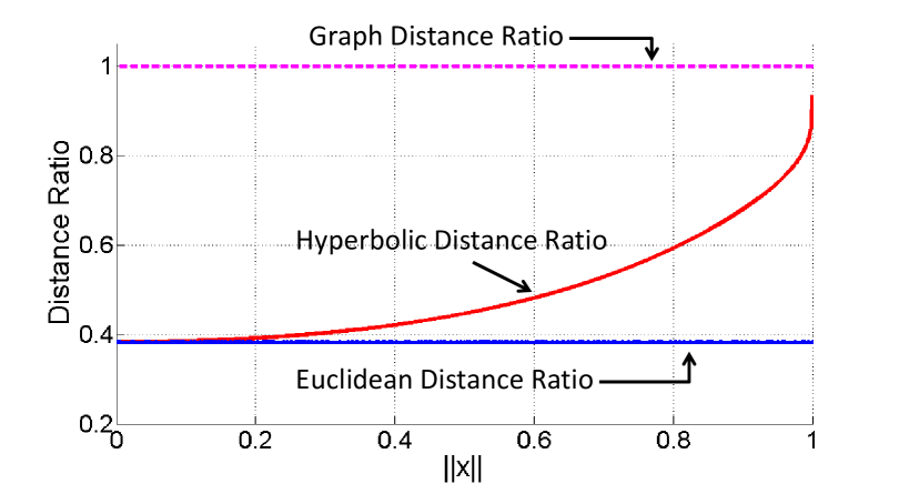
Figure 1: Geodesics and distances in the Poincaré disk. As $x$ and $y$ move towards the outside of the disk (i.e., letting $\|x\|,\|y\|\rightarrow 1$), the distance $d_{H}(x,y)$ approaches $d_{H}(x,O)+d_{H}(O,y)$.

Hyperbolic spaces

The Poincaré disk $\mathbb{H}_{2}$ is a two-dimensional model of hyperbolic geometry with points located in the interior of the unit disk, as shown in Figure 1. A natural generalization of $\mathbb{H}_{2}$ is the Poincaré ball $\mathbb{H}_{r}$, with elements inside the unit ball. The Poincaré models offer several useful properties, chief among which is mapping conformally to Euclidean space. That is, angles are preserved between hyperbolic and Euclidean space. Distances, on the other hand, are not preserved, but are given by

$$d_{H}(x,y)=\text{acosh}\left(1+2\frac{\lVert{x}-{y}\rVert^{2}}{(1-\lVert{x}\rVert^{2})(1-\lVert{y}\rVert^{2})}\right).$$

There are some potentially unexpected consequences of this formula, and a simple example gives intuition about a key technical property that allows hyperbolic space to embed trees. Consider three points: the origin $0$, and points $x$ and $y$ with $\|x\|=\|y\|=t$ for some $t>0$. As shown on the right of Figure 1, as $t\rightarrow 1$ (i.e., the points move towards the outside of the disk), in flat Euclidean space, the ratio $\frac{d_{E}(x,y)}{d_{E}(x,0)+d_{E}(0,y)}$ is constant with respect to $t$ (blue curve). In contrast, the ratio $\frac{d_{H}(x,y)}{d_{H}(x,0)+d_{H}(0,y)}$ approaches 1, or, equivalently, the distance $d_{H}(x,y)$ approaches $d_{H}(x,0)+d_{H}(0,y)$ (red and pink curves). That is, the shortest path between $x$ and $y$ is almost the same as the path through the origin. This is analogous to the property of trees in which the shortest path between two sibling nodes is the path through their parent. This tree-like nature of hyperbolic space is the key property exploited by embeddings. Moreover, this property holds for arbitrarily small angles between $x$ and $y$.

Lines and geodesics

There are two types of geodesics (shortest paths) in the Poincaré disk model of hyperbolic space: segments of circles that are orthogonal to the disk surface, and disk diameters [3]. Our algorithms and proofs make use of a simple geometric fact: isometric reflection across geodesics (preserving hyperbolic distances) is represented in this Euclidean model as a circle inversion. A particularly important reflection associated with each point $x$ is the one that takes $x$ to the origin [3, p. 268].

Embeddings and fidelity measures

An embedding is a mapping $f:U\rightarrow V$ for spaces $U,V$ with distances $d_{U},d_{V}$. We measure the quality of embeddings with several fidelity measures, presented here from most local to most global.

Recent work [28] proposes using the mean average precision (MAP). For a graph $G=(V,E)$, let $a\in V$ have neighborhood $\mathcal{N}_{a}=\{b_{1},b_{2},\ldots,b_{\operatorname{deg}(a)}\}$, where $\operatorname{deg}(a)$ denotes the degree of $a$. In the embedding $f$, consider the points closest to $f(a)$, and define $R_{a,b_{i}}$ to be the smallest set of such points that contains $b_{i}$ (that is, $R_{a,b_{i}}$ is the smallest set of nearest points required to retrieve the $i$th neighbor of $a$ in $f$). Then, the MAP is defined to be

$$\text{MAP}(f)=\frac{1}{|V|}\sum_{a\in V}\frac{1}{|\mathcal{N}_{a}|}\sum_{i=1}^{|\mathcal{N}_{a}|}\text{Precision}(R_{a,b_{i}})=\frac{1}{|V|}\sum_{a\in V}\frac{1}{\operatorname{deg}(a)}\sum_{i=1}^{|\mathcal{N}_{a}|}\frac{\left|\mathcal{N}_{a}\cap R_{a,b_{i}}\right|}{\left|R_{a,b_{i}}\right|}.$$

We have $\text{MAP}(f)\leq 1$, with equality as the best case. Note that MAP is not concerned with the underlying distances at all, but only the ranks between the distances of immediate neighbors. It is a local metric.

The standard metric for graph embeddings is distortion $D$. For an $n$ point embedding,

$$D(f)=\frac{1}{\binom{n}{2}}\left(\sum_{u,v\in U:u\neq v}\frac{|d_{V}(f(u),f(v))-d_{U}(u,v)|}{d_{U}(u,v)}\right).$$

The best distortion is $D(f)=0$, preserving the edge lengths exactly. This is a global metric, as it depends directly on the underlying distances rather than the local relationships between distances. A variant of this, the worst-case distortion $D_{\mathrm{wc}}$, is the metric defined by

$$D_{\mathrm{wc}}(f)=\frac{\max_{u,v\in U:u\neq v}d_{V}(f(u),f(v))/d_{U}(u,v)}{\min_{u,v\in U:u\neq v}d_{V}(f(u),f(v))/d_{U}(u,v)}.$$

That is, the wost-case distortion is the ratio of the maximal expansion and the minimal contraction of distances. Note that scaling the unit distance does not affect $D_{\mathrm{wc}}$. The best worst-case distortion is $D_{\mathrm{wc}}(f)=1$.

The intended application of the embedding informs the choice of metric. For applications where the underlying distances are important, distortion is useful. On the other hand, if only rankings matter, MAP may suffice. This choice is important: as we shall see, different embedding algorithms implicitly target different metrics.

Reconstruction and learning

In the case where we lack a full set of distances, we can deal with the missing data in one of two ways. First, we can use the triangle inequality to recover the missing distances. Second, we can access the scaled Euclidean distances (the inside of the $\operatorname{acosh}$ in $d_{H}(x,y)$), and then the resulting matrix can be recovered with standard matrix completion techniques [4]. Afterwards, we can proceed to compute an embedding using any of the approaches discussed in this paper. We quantify the error introduced by this process experimentally in Section 5.

3 Combinatorial Constructions

We first focus on hyperbolic tree embeddings—a natural approach considering the tree-like behavior of hyperbolic space. We review the embedding of Sarkar [32] to higher dimensions. We then provide novel analysis about the precision of the embeddings that reveals fundamental limits of hyperbolic embeddings. In particular, we characterize the bits of precision needed for hyperbolic representations. We then extend the construction to $r$ dimensions, and we propose to use Steiner nodes to better embed general graphs as trees building on a condition from I. Abraham et al. [18].

Embedding trees

The nature of hyperbolic space lends itself towards excellent tree embeddings. In fact, it is possible to embed trees into the Poincaré disk $\mathbb{H}_{2}$ with arbitrarily low distortion [32]. Remarkably, trees cannot be embedded into Euclidean space with arbitrarily low distortion for any number of dimensions. These notions motivate the following two-step process for embedding hierarchies into hyperbolic space.

1. Embed the graph $G=(V,E)$ into a tree $T$,

2. Embed $T$ into the Poincaré ball $\mathbb{H}_{d}$.

We refer to this process as the combinatorial construction. Note that we are not required to minimize a loss function. We begin by describing the second stage, where we extend an elegant construction from Sarkar [32].

3.1 Sarkar’s Construction

Algorithm 1 implements a simple embedding of trees into $\mathbb{H}_{2}$. The algorithm takes as input a scaling factor $\tau$ a node $a$ (of degree $\operatorname{deg}(a)$) from the tree with parent node $b$. Suppose $a$ and $b$ have already been embedded into $\mathbb{H}_{2}$ and have corresponding embedded vectors $f(a)$ and $f(b)$. The algorithm places the children $c_{1},c_{2},\ldots,c_{\operatorname{deg}(a)-1}$ into $\mathbb{H}_{2}$ through a two-step process.

First, $f(a)$ and $f(b)$ are reflected across a geodesic (using circle inversion) so that $f(a)$ is mapped onto the origin $0$ and $f(b)$ is mapped onto some point $z$. Next, we place the children nodes to vectors $y_{1},\ldots,y_{d-1}$ equally spaced around a circle with radius $\frac{e^{\tau}-1}{e^{\tau}+1}$ (which is a circle of radius $\tau$ in the hyperbolic metric), and maximally separated from the reflected parent node embedding $z$. Lastly, we reflect all of the points back across the geodesic. Note that the isometric properties of reflections imply that all children are now at hyperbolic distance exactly $\tau$ from $f(a)$.

1:  Input: Node $a$ with parent $b$, children to place $c_{1},c_{2},\ldots,c_{\operatorname{deg}(a)-1}$, partial embedding $f$ containing an embedding for $a$ and $b$, scaling factor $\tau$

2:  $(0,z)\leftarrow\operatorname{reflect}_{f(a)\rightarrow 0}(f(a),f(b))$

3:  $\theta\leftarrow\operatorname{arg}(z)$        {angle of $z$ from x-axis in the plane}

4:  for $i\in\{1,\ldots,\operatorname{deg}(a)-1\}$ do

5:     $y_{i}\leftarrow\left(\frac{e^{\tau}-1}{e^{\tau}+1}\cdot\cos\left(\theta+\frac{2\pi i}{\operatorname{deg}(a)}\right),\frac{e^{\tau}-1}{e^{\tau}+1}\cdot\sin\left(\theta+\frac{2\pi i}{\operatorname{deg}(a)}\right)\right)$

6:  end for

7:  $(f(a),f(b),f(c_{1}),\ldots,f(c_{\operatorname{deg}(a)-1}))\leftarrow\operatorname{reflect}_{0\rightarrow f(a)}(0,z,y_{1},\ldots,y_{\operatorname{deg}(x)-1})$

8:  Output: Embedded $\mathbb{H}_{2}$ vectors $f(c_{1}),f(c_{2}),\ldots,f(c_{\operatorname{deg}(a)-1})$

Algorithm 1 Sarkar’s Construction

To embed the entire tree, we place the root at the origin $O$ and its children in a circle around it (as in Step 5 of Algorithm 1), then recursively place their children until all nodes have been placed. Notice this construction runs in linear time.

3.2 Analyzing Sarkar’s Construction

The Voronoi cell around a node $a\in T$ consists of points $x\in\mathbb{H}_{2}$ such that $d_{H}(f(a),x)\leq d_{H}(f(b),x)$ for all $b\in T$ distinct from $a$. That is, the cell around $a$ includes all points closer to $f(a)$ than to any other embedded node of the tree. Sarkar’s construction produces Delauney embeddings: embeddings where the Voronoi cells for points $a$ and $b$ touch only if $a$ and $b$ are neighbors in $T$. Thus this embedding will preserve neighborhoods.

A key technical idea exploited by Sarkar [32] is to scale all the edges by a factor $\tau$ before embedding. We can then recover the original distances by dividing by $\tau$. This transformation exploits the fact that hyperbolic space is not scale invariant. Sarkar’s construction always captures neighbors perfectly, but Figure 1 implies that increasing the scale preserves the distances between farther nodes better. Indeed, if one sets $\tau=\frac{1+\varepsilon}{\varepsilon}\left(2\log\frac{\operatorname{deg}_{\max}}{\pi/2}\right)$, then the worst-case distortion $D$ of the resulting embedding is no more than $1+\varepsilon$. For trees, Sarkar’s construction has arbitrarily high fidelity. However, this comes at a cost: the scaling $\tau$ affects the bits of precision required. In fact, we will show that the precision scales logarithmically with the degree of the tree—but linearly with the maximum path length. We use this to better understand the situations in which hyperbolic embeddings obtain high quality.

How many bits of precision do we need to represent points in $\mathbb{H}_{2}$? If $x\in\mathbb{H}_{2}$, then $\|x\|<1$, so we need sufficiently many bits so that $1-\|x\|$ will not be rounded to zero. This requires roughly $-\log(1-\|x\|)=\log\frac{1}{1-\|x\|}$ bits. Say we are embedding two points $x,y$ at distance $d$. As described in the background, there is an isometric reflection that takes a pair of points $(x,y)$ in $\mathbb{H}_{2}$ to $(0,z)$ while preserving their distance, so without loss of generality we have that

$$d=d_{H}(x,y)=d_{H}(0,z)=\operatorname{acosh}\left(1+2\frac{\|z\|^{2}}{1-\|z\|^{2}}\right).$$

Rearranging the terms, we have

$$\frac{\cosh(d)+1}{2}=\frac{1}{1-\|z\|^{2}}\geq\frac{1/2}{1-\|z\|}.$$

Thus, the number of bits we want so that $1-\|z\|$ will not be rounded to zero is $\log(\cosh(d)+1)$. Since $\cosh(d)=(\exp(d)+\exp(-d))/2$, this is roughly $d$ bits. That is, in hyperbolic space, we need about $d$ bits to express distances of $d$ (rather than $\log d$ as we would in Euclidean space). This result will be of use below.

Now we consider the largest distance in the embeddings produced by Algorithm 1. If the longest path in the tree is $\ell$, and each edge has length $\tau=\frac{1}{\varepsilon}\left(2\log\frac{\operatorname{deg}_{\text{max}}}{\pi/2}\right)$, the largest distance is $O(\frac{\ell}{\varepsilon}\log\operatorname{deg}_{\text{max}})$, and we require this number of bits for the representation.

We interpret this expression. Note that $\operatorname{deg}_{\max}$ is inside the $\log$ term, so that a bushy tree is not penalized much in precision. On the other hand, the longest path length $\ell$ is not, so that hyperbolic embeddings struggle with long paths. Moreover, by selecting an explicit graph, we derive a matching lower bound, concluding that to achieve a distortion $\varepsilon$, any construction requires $\Omega\left(\frac{\ell}{\varepsilon}\log(\text{deg}_{\max})\right)$ bits, which matches the upper bound of the combinatorial construction. The argument follows from selecting a graph consisting of $m(\text{deg}_{\max}+1)$ nodes in a tree with a single root and $\text{deg}_{\max}$ chains each of length $m$. The proof of this result is described in Appendix D.

3.3 Improving the Construction

Our next contribution is a generalization of the construction from the disk $\mathbb{H}_{2}$ to the ball $\mathbb{H}_{r}$. Our construction follows the same line as Algorithm 1, but since we have $r$ dimensions, the step where we place children spaced out on a circle around their parent now uses a hypersphere.

Spacing out points on the hypersphere is a classic problem known as spherical coding [7]. As we shall see, the number of children that we can place for a particular angle grows with the dimension. Since the required scaling factor $\tau$ gets larger as the angle decreases, we can reduce $\tau$ for a particular embedding by increasing the dimension. Note that increasing the dimension helps with bushy trees (large $\operatorname{deg}_{\max}$), but has limited effect on tall trees with small $\operatorname{deg}_{\max}$. We show

Proposition 3.1.

The generalized $\mathbb{H}_{r}$ combinatorial construction has distortion at most $1+\varepsilon$ and requires at most $O(\frac{1}{\varepsilon}\frac{\ell}{r}\log\operatorname{deg}_{\max})$ bits to represent a node component for $r\leq(\log\operatorname{deg}_{\max})+1$, and $O(\frac{1}{\varepsilon}\ell)$ bits for $r>(\log\operatorname{deg}_{\max})+1$.

The algorithm for the generalized $\mathbb{H}_{r}$ combinatorial construction replaces Step 5 in Algorithm 1 with a node placement step based on ideas from coding theory. The children are placed at the vertices of a hypercube inscribed into the unit hypersphere (and afterwards scaled by $\tau$). Each component of a hypercube vertex has the form $\frac{\pm 1}{\sqrt{r}}$. We index these points using binary sequences ${a}\in\{0,1\}^{r}$ in the following way:

$${x}_{a}=\left(\frac{(-1)^{a_{1}}}{\sqrt{r}},\frac{(-1)^{a_{2}}}{\sqrt{r}},\ldots,\frac{(-1)^{a_{r}}}{\sqrt{r}}\right).$$

We can space out the children by controlling the distances between the children. This is done in turn by selecting a set of binary sequences with a prescribed minimum Hamming distance—a binary error-correcting code—and placing the children at the resulting hypercube vertices. We provide more details on this technique and our choice of code in the appendix.

3.4 Embedding into Trees

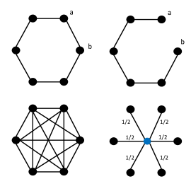
Figure 2: Top. Cycles are a challenge for tree embeddings: $d_{G}(a,b)$ goes from $1$ to $5$. Bottom. Steiner nodes can help: adding a node (blue) and weighting edges maintains the pairwise distances.

We revisit the first step of the construction: embedding graphs into trees. There are fundamental limits to how well graphs can be embedded into trees; in general, breaking long cycles inevitably adds distortion, as shown in Figure 2. We are inspired by a measure of this limit, the $\delta$-4 points condition introduced in I. Abraham et al. [18]. A graph on $n$ nodes that satisfies the $\delta$-4 points condition has distortion at most $(1+\delta)^{c_{1}\log n}$ for some constant $c_{1}$. This result enables our end-to-end embedding to achieve a distortion of at most

$$D(f)\leq(1+\delta)^{c_{1}\log n}(1+\varepsilon).$$

The result in I. Abraham et al. [18] builds a tree with Steiner nodes. These additional nodes can help control the distances in the resulting tree.

Example 3.1.

Embed a complete graph on $\{1,2,\ldots,n\}$ into a tree. The tree will have a central node, say 1, w.l.o.g., connected to every other node; the shortest paths between pairs of nodes in $\{2,\ldots,n\}$ go from distance 1 in the graph to distance 2 in the tree. However, we can introduce a Steiner node $n+1$ and connect it to all of the nodes, with edge weights of $\frac{1}{2}$. This is shown in Figure 2. The distance between any pair of nodes in $\{1,\ldots,n\}$ remains 1.

Note that introducing Steiner nodes can produce a weighted tree, but Algorithm 1 readily extends to the case of weighted trees by modifying Step 5. We propose using the Steiner tree algorithm in I. Abraham et al. [18] (used to achieve the distortion bound) for real embeddings, and we rely on it for our experiments in Section 5. In summary, the key takeaways of our analysis in this section are:

• There is a fundamental tension between precision and quality in hyperbolic embeddings.

• Hyperbolic embeddings have an exponential advantage in space compared to Euclidean embeddings for short, bushy hierarchies, but will have less of an advantage for graphs that contain long paths.

• Choosing an appropriate scaling factor $\tau$ is critical for quality. Later, we will propose to learn this scale factor automatically for computing embeddings in PyTorch.

• Steiner nodes can help improve embeddings of graphs.

4 Hyperbolic Multidimensional Scaling

In this section, we explore a fundamental and more general question than we did in the previous section: if we are given the pairwise distances arising from a set of points in hyperbolic space, can we recover the points? The equivalent problem for Euclidean distances is solved with multidimensional scaling (MDS). The goal of this section is to analyze the hyperbolic MDS (h-MDS) problem. We describe and overcome the additional technical challenges imposed by hyperbolic distances, and show that exact recovery is possible and interpretable. Afterwards we propose a technique for dimensionality reduction using principal geodesics analysis (PGA) that provides optimization guarantees. In particular, this addresses the shortcomings of h-MDS when recovering points that do not exactly lie on a hyperbolic manifold.

4.1 Exact Hyperbolic MDS

Suppose that there is a set of hyperbolic points $x_{1},\dots,x_{n}\in\mathbb{H}_{r}$, embedded in the Poincaré ball and written $X\in\mathbb{R}^{n\times r}$ in matrix form. We observe all the pairwise distances $d_{i,j}=d_{H}(x_{i},x_{j})$, but do not observe $X$: our goal is use the observed $d_{i,j}$’s to recover $X$ (or some other set of points with the same pairwise distances $d_{i,j}$).

The MDS algorithm in the Euclidean setting makes an important centering assumption. That is it assumes the points have mean $0$, and it turns out that if an exact embedding for the distances exists, it can be recovered from a matrix factorization. In other words, Euclidean MDS always recovers a centered embedding.

In hyperbolic space, the same algorithm does not work, but we show that it is possible to find an embedding centered at a different mean. More precisely, we introduce a new mean which we call the pseudo-Euclidean mean, that behaves like the Euclidean mean in that it enables recovery through matrix factorization. Once the points are recovered in hyperbolic space, they can be recentered around a more canonical mean by translating it to the origin.

Algorithm 2 is our complete algorithm, and for the remainder of this section we will describe how and why it works. We first describe the hyperboloid model, an alternate but equivalent model of hyperbolic geometry in which h-MDS is simpler. Of course, we can easily convert between the hyperboloid model and the Poincaré ball model we have used thus far. Next, we show how to reduce the problem to a standard PCA problem, which recovers an embedding centered at the points’ pseudo-Euclidean mean. Finally, we discuss the meaning and implications of centering and prove that the algorithm preserves submanifolds as well—that is, if there is an exact embedding in $k<r$ dimensions centered at their canonical mean, then our algorithm will recover them.

The hyperboloid model

Define $Q$ to be the diagonal matrix in $\mathbb{R}^{r+1}$ where $Q_{00}=1$ and $Q_{ii}=-1$ for $i>0$. For a vector $x\in\mathbb{R}^{r+1}$, $x^{T}Qx$ is called the Minkowski quadratic form. The hyperboloid model is defined as

$$\mathbb{M}_{r}=\left\{x\in\mathbb{R}^{r+1}\middle|x^{T}Qx=1\land x_{0}>0\right\}.$$

This manifold is endowed with a distance measure

$$d_{H}(x,y)=\operatorname{acosh}(x^{T}Qy).$$

As a notational convenience, for a point $x\in\mathbb{M}_{r}$ we will let $x_{0}$ denote $0$th coordinate $e_{0}^{T}x$, and let $\vec{x}\in\mathbb{R}^{r}$ denote the rest of the coordinates. Notice that $x_{0}$ is just a function of $\vec{x}$ (in fact, $x_{0}=\sqrt{1+\|\vec{x}\|^{2}}$), and so we can equivalently consider just $\vec{x}$ as being a member of a model of hyperbolic space: this model is sometimes known as the Gans model. With this notation, the Minkowski quadratic form can be simplified to $x^{T}Qy=x_{0}y_{0}-\vec{x}^{T}\vec{y}$.

A new mean

We introduce the new mean that we will use. Given points $x_{1},x_{2},\ldots,x_{n}\in\mathbb{M}_{r}$ in hyperbolic space, define a variance term

$$\Psi(z;x_{1},x_{2},\ldots,x_{n})=\sum_{i=1}^{n}\sinh^{2}(d_{H}(x_{i},z)).$$

Using this, we define a pseudo-Euclidean mean to be any local minimum of this expression. Notice that this average is independent of the model of hyperbolic space that we are using, since it only is defined in terms of the hyperbolic distance function $d_{H}$.

Lemma 4.1.

Define the matrix $X\in\mathbb{R}^{n\times r}$ such that $X^{T}e_{i}=\vec{x}_{i}$ and the vector $u\in\mathbb{R}^{n}$ such that $u_{i}=x_{0,i}$. Then

$$\left.\nabla_{\vec{z}}\Psi(z;x_{1},x_{2},\ldots,x_{n})\right|_{\vec{z}=0}=-2\sum_{i=1}^{n}x_{0,i}\vec{x}_{i}=-2X^{T}u.$$

This means that $0$ is a pseudo-Euclidean mean if and only if $0=X^{T}u$. Call some hyperbolic points $x_{1},\ldots,x_{n}$ pseudo-Euclidean centered if their average is $0$ in this sense: i.e. if $X^{T}u=0$. We can always center a set of points without affecting their pairwise distances by simply finding their average, and then sending it to $0$ through an isometry.

Recovery via matrix factorization

Suppose that there exist points $x_{1},x_{2},\ldots,x_{n}\in\mathbb{M}_{r}$ for which we observe their pairwise distances $d_{H}(x_{i},x_{j})$. From these, we can compute the matrix $Y$ such that

$$Y_{i,j}=\cosh\left(d_{H}(x_{i},x_{j})\right)=x_{i}^{T}Qx_{j}=x_{0,i}x_{0,j}-\vec{x_{i}}^{T}\vec{x_{j}}.$$ (1)

Furthermore, defining $X$ and $u$ as in Lemma 4.1, then we can write $Y$ in matrix form as

$$Y=uu^{T}-XX^{T}.$$ (2)

Without loss of generality, we can suppose that the points we are trying to recover, $x_{1},\ldots,x_{n}$, are centered at their pseudo-Euclidean mean, so that $X^{T}u=0$ by Lemma 4.1.

This implies that $u$ is an eigenvector of $Y$ with positive eigenvalue, and the rest of $Y$’s eigenvalues are negative. Therefore an eigendecomposition of $Y$ will find $u,\hat{X}$ such that $Y=uu^{T}-\hat{X}\hat{X}^{T}$, i.e. it will directly recover $X$ up to rotation.

In fact, running PCA on $-Y=X^{T}X-uu^{T}$ to find the $n$ most significant non-negative eigenvectors will recover $X$ up to rotation, and then $u$ can be found by leveraging the fact that $x_{0}=\sqrt{1+\|\vec{x}\|^{2}}$.

This leads to Algorithm 2, with optional post-processing steps for converting the embedding to the Poincaré ball model and for re-centering the points.

A word on centering

The MDS algorithm in Euclidean geometry returns points centered at their Karcher mean $z$, which is a point minimizing $\sum d^{2}(z,x_{i})$ (where $d$ is the distance metric). The Karcher center is particularly useful for interpreting dimensionality reduction; for example, we use the analogous hyperbolic Karcher mean to perform PGA in Section 4.2.

Although Algorithm 2 returns points centered at their pseudo-Euclidean mean instead of their Karcher mean, they can be easily recentered by finding their Karcher mean and reflecting it onto the origin. Furthermore, we show that Algorithm 2 preserves the dimension of the embedding. More precisely, we prove Lemma 4.2 in Appendix E.

Lemma 4.2.

If a set of points lie in a dimension-$k$ geodesic submanifold, then both their Karcher mean and their pseudo-Euclidean mean lie in the same submanifold.

This implies that centering with the pseudo-Euclidean mean preserves geodesic submanifolds: If it is possible to embed distances in a dimension-$k$ geodesic submanifold centered and rooted at a Karcher mean, then it is also possible to embed the distances in a dimension-$k$ submanifold centered and rooted at a pseudo-Euclidean mean, and vice versa.

Algorithm 2

1:  Input: Distance matrix $d_{i,j}$ and rank $r$

2:  Compute scaled distance matrix $Y_{i,j}=\cosh(d_{i,j})$

3:  $X\rightarrow\text{PCA}(-Y,r)$

4:  Project $X$ from hyperboloid model to Poincaré model: $x\to\frac{x}{1+\sqrt{1+\|x\|^{2}}}$

5:  If desired, center $X$ at a different mean (e.g. the Karcher mean)

6:  return $X$

4.2 Reducing Dimensionality with PGA

Sometimes we are given a high-rank embedding (resulting from h-MDS, for example), and wish to find a lower-rank version. In Euclidean space, one can get the optimal lower rank embedding by simply discarding components. However, this may not be the case in hyperbolic space. Motivated by this, we study dimensionality reduction in hyperbolic space.

As hyperbolic space does not have a linear subspace structure like Euclidean space, we need to define what we mean by lower-dimensional. We follow Principal Geodesic Analysis [12], [17]. Consider an initial embedding with points $x_{1},\dots,x_{n}\in\mathbb{H}_{2}$ and let $d_{H}:\mathbb{H}_{2}\times\mathbb{H}_{2}\to\mathbb{R}_{+}$ be the hyperbolic distance. Suppose we want to map this embedding onto a one-dimensional subspace. (Note that we are considering a two-dimensional embedding and one-dimensional subspace here for simplicity, and these results immediately extend to higher dimensions.) In this case, the goal of PGA is to find a geodesic $\gamma:[0,1]\to\mathbb{H}_{2}$ that passes through the mean of the points and that minimizes the squared error (or variance):

$$f(\gamma)=\sum_{i=1}^{n}\min_{t\in[0,1]}d_{H}(\gamma(t),x_{i})^{2}.$$

This expression can be simplified significantly and reduced to a minimization in Euclidean space. First, we find the mean of the points, the point $\bar{x}$ which minimizes $\sum_{i=1}^{n}d_{H}(\bar{x},x_{i})^{2}$; this definition in terms of distances generalizes the mean in Euclidean space. Next, we reflect all the points $x_{i}$ so that their mean is $0$ in the Poincaré disk model; we can do this using a circle inversion that maps $\bar{x}$ onto $0$. In the Poincaré disk model, a geodesic through the origin is a Euclidean line, and the action of the reflection across this line is the same in both Euclidean and hyperbolic space. Coupled with the fact that reflections are isometric, if $\gamma$ is a line through $0$ and $R_{\gamma}$ is the reflection across $\gamma$, we have

$$d_{H}(\gamma,x)=\min_{t\in[0,1]}d_{H}(\gamma(t),x)=\frac{1}{2}d_{H}(R_{l}x,x).$$

Combining this with the Euclidean reflection formula and the hyperbolic metric produces

$$f(\gamma)=\frac{1}{4}\sum_{i=1}^{n}\operatorname{acosh}^{2}\left(1+\frac{8d_{E}(\gamma,x_{i})^{2}}{(1-\|x_{i}\|^{2})^{2}}\right),$$

in which $d_{E}$ is the Euclidean distance from a point to a line. If we define $w_{i}=\sqrt{8}x_{i}/(1-\|x_{i}\|^{2})$ this reduces to the simplified expression

$$f(\gamma)=\frac{1}{4}\sum_{i=1}^{n}\operatorname{acosh}^{2}\left(1+d_{E}(\gamma,w_{i})^{2}\right).$$

Notice that the loss function is not convex. We observe that there can be multiple local minima that are attractive and stable, in contrast to PCA. Figure 3 illustrates this nonconvexity on a simple dataset in $\mathbb{H}_{2}$ with only four examples. This makes globally optimizing the objective difficult.

Figure 3: The PGA objective of an example task where the input dataset in the Poincaré disk is $x_{1}=(0.8,0)$, $x_{2}=(-0.8,0)$, $x_{3}=(0,0.7)$ and $x_{4}=(0,-0.7)$. Note the presence of non-optimal local minima, unlike PCA.

Nevertheless, there will always be a region $\Omega$ containing a global optimum $\gamma^{*}$ that is convex and admits an efficient projection, and where $f$ is convex when restricted to $\Omega$. Thus it is possible to build a gradient descent-based algorithm to recover lower-dimensional subspaces: for example, we built a simple optimizer in PyTorch. We also give a sufficient condition on the data for $f$ above to be convex.

Lemma 4.3.

For hyperbolic PGA if for all $i$,

$$\operatorname{acosh}^{2}\left(1+d_{E}(\gamma,w_{i})^{2}\right)<\min\left(1,\frac{1}{3}\|w_{i}\|^{2}\right)$$

then $f$ is locally convex at $\gamma$.

As a result, if we initialize in and optimize over a region that contains $\gamma^{*}$ and where the condition of Lemma 4.3 holds, then gradient descent will be guaranteed to converge to $\gamma^{*}$. We can turn this result around and read it as a recovery result: if the noise is bounded in this regime, then we are able to provably recover the correct low-dimensional embedding.

5 Experiments

Dataset	Nodes	Edges	Comment
Bal. Tree	40	39	Tree
Phy. Tree	344	343	Tree
CS PhDs	1025	1043	Tree-like
WordNet	74374	75834	Tree-like
Diseases	516	1188	Dense
Gr-QC	4158	13428	Dense

Table 1: Datasets Statistics.

Dataset	C-$\mathbb{H}_{2}$	FB $\mathbb{H}_{5}$	FB $\mathbb{H}_{200}$
WordNet	0.989	0.823*	0.87*

Table 2: MAP measure for WordNet embedding compared to values in Nickel and Kiela [28]. Closer to 1 is better.

Dataset	C-$\mathbb{H}_{2}$	FB $\mathbb{H}_{2}$	h-MDS	PyTorch	PWS	PCA	FB
Bal. Tree	0.013	0.425	0.077	0.034	0.020	0.496	0.236
Phy. Tree	0.006	0.832	0.039	0.237	0.092	0.746	0.583
CS PhDs	0.286	0.542	0.149	0.298	0.187	0.708	0.336
Diseases	0.147	0.410	0.111	0.080	0.108	0.595	0.764
Gr-QC	0.354	-	0.530	0.125	0.134	0.546	-

Table 3: Distortion measures using combinatorial and h-MDS techniques, compared against PCA and results from Nickel and Kiela [28]. Closer to 0 is better.

Dataset	C-$\mathbb{H}_{2}$	FB $\mathbb{H}_{2}$	h-MDS	PyTorch	PWS	PCA	FB
Bal. Tree	1.0	0.846	1.0	1.0	1.0	1.0	0.859
Phy. Tree	1.0	0.718	0.675	0.951	0.998	1.0	0.811
CS PhDs	0.991	0.567	0.463	0.799	0.945	0.541	0.78
Diseases	0.822	0.788	0.949	0.995	0.897	0.999	0.934
Gr-QC	0.696	-	0.710	0.733	0.504	0.738	0.999∗

Table 4: MAP measures using combinatorial and h-MDS techniques, compared against PCA. Closer to 1 is better.

We evaluate the proposed approaches and compare against existing methods. We hypothesize that for tree-like data, the combinatorial construction offers the best performance. For general data, we expect h-MDS to produce the lowest distortion, while it may have low MAP due to precision limitations. We anticipate that dimension is a critical factor (outside of the combinatorial construction). Finally, we expect that the MAP of h-MDS techniques can be improved by learning the correct scale and weighting the loss function as suggested in earlier sections. In the Appendix, we report on additional datasets, parameters found by the combinatorial construction, and the effect of hyperparameters.

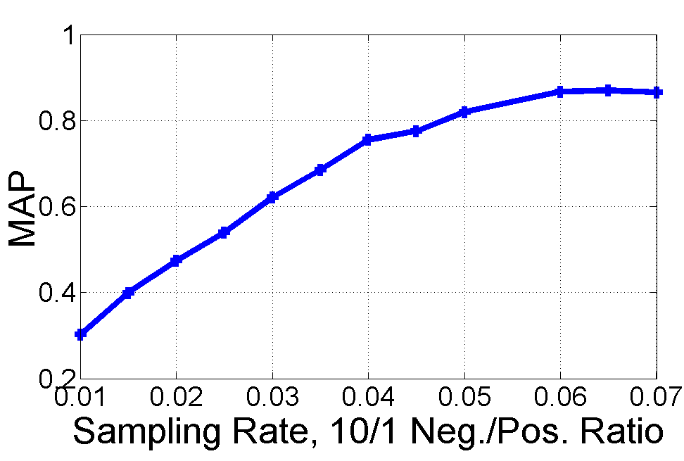
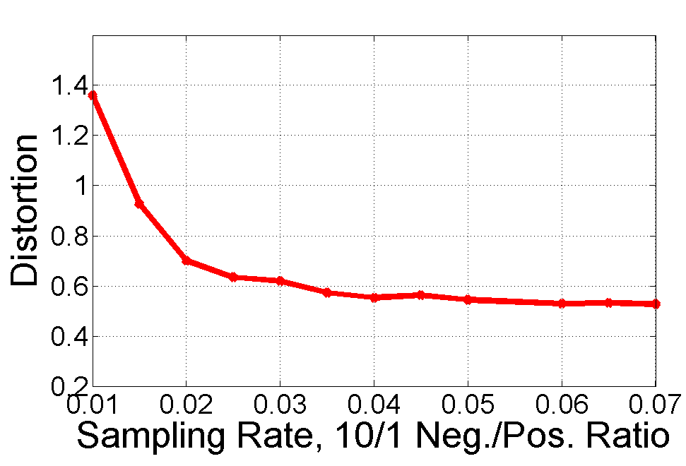
Figure 4: Learning from incomplete information. The distance matrix is sampled, completed, and embedded.

Rank	No Scale	Learned Scale	Exp. Weighting
50	0.481	0.508	0.775
100	0.688	0.681	0.882
200	0.894	0.907	0.963

Table 5: Ph.D. dataset. Improved MAP performance of PyTorch implementation using a modified PGA-like loss function.

Datasets

We consider trees, tree-like hierarchies, and graphs that are not tree-like. First, we consider hierarchies that form trees: fully-balanced trees along with phylogenetic trees expressing genetic heritage (of mosses growing in urban environments [16], available from [31]). Similarly, we used hierarchies that are nearly tree-like: WordNet hypernym (the largest connected component from Nickel and Kiela [28]) and a graph of Ph.D. advisor-advisee relationships [10]. Also included are datasets that vary in their tree nearness, such as biological sets involving disease relationships [14] and protein interactions in yeast bacteria [20], both available from [30]. We also include the collaboration network formed by authorship relations for papers submitted to the general relativity and quantum cosmology (Gr-QC) arXiv [26].

Approaches

Combinatorial embeddings into $\mathbb{H}_{2}$ are done using Steiner trees generated from a randomly selected root for the $\varepsilon=0.1$ precision setting; others are considered in the Appendix. We performed h-MDS in floating point precision. We also include results for our PyTorch implementation of an SGD-based algorithm (described later), as well as a warm start version initialized with the high-dimensional combinatorial construction. We compare against classical MDS (i.e., PCA), and the optimization-based approach Nickel and Kiela [28], which we call FB. The experiments for h-MDS, PyTorch SGD, PCA, and FB used dimensions of 2,5,10,50,100,200; we recorded the best resulting MAP and distortion. Due to the large scale, we did not replicate the best FB numbers on large graphs (i.e., Gr-QC and WordNet). As a result, we report their best published MAP numbers for comparison (their work does not report distortion). These entries are marked with an asterisk. For the WordNet graph we use a random BFS tree rather than a Steiner tree. Moreover, for comparison against FB (which computes the transitive closure), we can use a weighted version of the graph that captures the ancestor relationships. The full details are in Appendix.

Quality

In Table 3, we report the distortion. As expected, when the graph is a tree or tree-like the combinatorial construction has exceedingly low distortion. Because h-MDS is meant to recover points exactly, we hypothesized that h-MDS would offer very low distortion on these datasets. We confirm this hypothesis: among h-MDS, PCA, and FB, h-MDS consistently offers the best (lowest) distortion, producing, for example, a distortion of $0.039$ on the phylogenetic tree dataset. We observe that the optimization-based approach works quite well for reducing distortion, and on tree-like datasets it is bolstered by appropriate initialization from the combinatorial construction.

Table 4 reports the MAP measure (this is shown in Table 2 for WordNet), which is a local measure. We expect that the combinatorial construction performs well for tree-like hierarchies. This is indeed the case: on trees and tree-like graphs, the MAP is close to 1, improving on approaches such as FB that rely on optimization. On larger graphs like WordNet, our approach yields a MAP of $0.989$–improving on the FB MAP result of $0.870$ at 200 dimensions. This is exciting because the combinatorial approach is deterministic and linear-time. In addition, it suggests that this refined understanding of hyperbolic embeddings may be used to improve the quality and runtime state of the art constructions. As expected, the MAP of the combinatorial construction decreases as the graphs are less tree-like. Interestingly, h-MDS solved in floating point indeed struggles with MAP. We separately confirmed that it is indeed due to precision using a high-precision solver, which obtains a perfect MAP—but uses 512 bits of precision. It may be possible to compensate for this with scaling, but we did not explore this possibility.

SGD-Based Algorithm

We also built an SGD-based algorithm implemented in PyTorch. Here the loss function is equivalent to the PGA loss, and so is continuously differentiable. We use this to verify two claims:

Learned Scale. In Table 5, we verify the importance of scaling that our analysis suggests; our implementation has a simple learned scale parameter. Moreover, we added an exponential weighting to the distances in order to penalize long paths, thus improving the local reconstruction. These techniques indeed improve the MAP; in particular, the learned scale provides a better MAP at lower rank. We hope these techniques can be useful in other embedding techniques.

Incomplete Information. To evaluate our algorithm’s ability to deal with incomplete information, we examine the quality of recovered solutions as we sample the distance matrix. We set the sampling rate of non-edges to edges at $10:1$ following Nickel and Kiela [28]. We examine the phylogenetic tree, which is full rank in Euclidean space. In Figure 4, we are able to recover a good solution with a small fraction of the entries for the phylogenetic tree dataset; for example, we sampled approximately $4\%$ of the graph but provide a MAP of $0.74$ and distortion of less than $0.6$. Understanding the sample complexity for this problem is an interesting theoretical question.

6 Conclusion and Future Work

Hyperbolic embeddings embed hierarchical information with high fidelity and few dimensions. We explored the limits of this approach by describing scalable, high quality algorithms. We hope the techniques here encourage more follow-on work on the exciting techniques of Nickel and Kiela [28], Chamberlain et al. [5]. As future work, we hope to explore how hyperbolic embeddings can be most effectively incorporated into downstream tasks and applications.

Appendix A Glossary of Symbols

Symbol	Used for
$x$, $y$, $z$	vectors in the Poincaré ball model of hyperbolic space
$d_{H}$	metric distance between two points in hyperbolic space
$d_{E}$	metric distance between two points in Euclidean space
$d_{U}$	metric distance between two points in metric space $U$
$d$	a particular distance value
$d_{i,j}$	the distance between the $i$th and $j$th points in an embedding
$\mathbb{H}_{r}$	the Poincaré ball model of $r$-dimensional Hyperbolic space
$r$	the dimension of a Hyperbolic space
$\mathbb{H}$	Hyperbolic space of an unspecified or arbitrary dimension
$\mathbb{M}_{r}$	the Minkowski (hyperboloid) model of $r$-dimensional Hyperbolic space
$f$	an embedding
$\mathcal{N}_{a}$	neighborhood around node $a$ in a graph
$R_{a,b}$	the smallest set of closest points to node $a$ in an embedding $f$ that contains node $b$
$\text{MAP}(f)$	the mean average precision fidelity measure of the embedding $f$
$D(f)$	the distortion fidelity measure of the embedding $f$
$D_{\mathrm{wc}}(f)$	the worst-case distortion fidelity measure of the embedding $f$
$G$	a graph, typically with node set $V$ and edge set $E$
$T$	a tree
$a,b,c$	nodes in a graph or tree
$\operatorname{deg}(a)$	the degree of node $a$
$\operatorname{deg}_{\max}$	maximum degree of a node in a graph
$\ell$	the longest path length in a graph
$\tau$	the scaling factor of an embedding
$\operatorname{reflect}_{x\rightarrow y}$	a reflection of $x$ onto $y$ in hyperbolic space
$\operatorname{arg}(z)$	the angle that the point $z$ in the plane makes with the $x$-axis
$X$	matrix of points in hyperbolic space
$Y$	matrix of transformed distances
$\gamma$	geodesic used in PGA
$w_{i}$	transformed points used in PGA

Table 6: Glossary of variables and symbols used in this paper.

Appendix B Related Work

Our study of representation tradeoffs for hyperbolic embeddings was motivated by exciting recent approaches towards such embeddings in Nickel and Kiela [28] and Chamberlain et al. [5]. Earlier efforts proposed using hyperbolic spaces for routing, starting with Kleinberg’s work on geographic routing [22]. Cvetkovski and Crovella [8] performed hyperbolic embeddings and routing for dynamic networks. Recognizing that the use of hyperbolic space for routing required a large number of bits to store the vertex coordinates, Eppstein and Goodrich [11] introduced a scheme for succinct embedding and routing in the hyperbolic plane. Another very recent effort also proposes using hyperbolic cones (similar to the cones that are the fundamental building block used in Sarkar [32] and our work) as a heuristic for embedding entailment relations, i.e. directed acyclic graphs [13]. The authors also propose to optimize on the hyperbolic manifold using its exponential map, as opposed to our approach of finding a closed form for the embedding should it exist (Section 4). An interesting avenue for future work is to compare both optimization methods empirically and theoretically, i.e., to understand the types of recovery guarantees under noise that such methods have.

There have been previous efforts to perform multidimensional scaling in hyperbolic space (the h-MDS problem), often in the context of visualization [25]. Most propose descent methods in hyperbolic space (e.g. [9], [37]) and fundamentally differ from ours. Arguably the most relevant is Wilson et al. [38], which mentions exact recovery as an intermediate result, but ultimately suggests a heuristic optimization. Our h-MDS analysis characterizes the recovered embedding and manifold and obtains the correctly centered one—a key issue in MDS. For example, this allows us to properly find the components of maximal variation. Furthermore, we discuss robustness to noise and produce optimization guarantees when a perfect embedding doesn’t exist.

Several papers have studied the notion of hyperbolicity of networks, starting with the seminal work on hyperbolic graphs Gromov [15]. More recently, Chen et al. [6] considered the hyperbolicity of small world graphs and tree-like random graphs. Abu-Ata and Dragan [1] performed a survey that examines how well real-world networks can be approximated by trees using a variety of tree measures and tree embedding algorithms. To motivate their study of tree metrics, I. Abraham et al. [18] computed a measure of tree likeness on a Internet infrastructure network.

We use matrix completion (closure) to perform embeddings with incomplete data. Matrix completion is a celebrated problem. Candes and Tao [4] derive bounds on the minimum number of entries needed for completion for a fixed rank matrix; they also introduce a convex program for matrix completion operating at near the optimal rate.

Principal geodesic analysis (PGA) generalizes principal components analysis (PCA) for the manifold setting. It was introduced and applied to shape analysis in [12] and extended to a probabilistic setting in [39]. There are other variants; the geodesic principal components analysis (GPCA) of Huckemann et al. [17] uses our loss function.

Appendix C Low-Level Formulation Details

We plan to release our PyTorch code, high precision solver, and other routines on Github. A few comments are helpful to understand the reformulation. In particular, we simply minimize the squared hyperbolic distance with a learned scale parameter, $\tau$, e.g., :

$$\min_{x_{1},\dots,x_{n},\tau}\sum_{1\leq i<j\leq n}\left(\tau d_{H}(x_{i},x_{j})-d_{i,j}\right)^{2}$$

We typically require that $\tau\geq 0.1$.

• On continuity of the derivative of the loss: Note that

  $$\partial_{x}\mathsf{acosh}(1+x)=\frac{1}{\sqrt{(1+x)^{2}-1}}=\frac{1}{\sqrt{x(x+2)}}\text{ hence }\lim_{x\to 0}\partial_{x}\mathsf{acosh}(1+x)=\infty.$$

  Thus, $\lim_{y\to x}\partial_{x}d_{H}(x,y)=\infty$. In particular, if two points happen to get near to one another during execution, gradient-based optimization becomes unstable. Note that $\exp\{\mathrm{acosh(1+x)}\}$ suffers from a similar issue, and is used in both [28, 5]. This change may increase numerical instability, and the public code for these approaches does indeed take steps like masking out updates to mitigate NaNs. In contrast, the following may be more stable:

  $$\partial_{x}\mathsf{acosh}(1+x)^{2}=2\frac{\mathsf{acosh}(1+x)}{\sqrt{x(x+2)}}\text{ and in particular }\lim_{x\to 0}\partial_{x}\mathsf{acosh}(1+x)^{2}=2$$

  The limits follows by simply applying L’Hopital’s rule. In turn, this implies the square formulation is continuously differentiable. Note that it is not convex.

• One challenge is to make sure the gradient computed by PyTorch has the appropriate curvature correction (the Riemannian metric), as is well explained by Nickel and Kiela [28]. The modification is straightforward: we create a subclass of nn.Parameter called Hyperbolic_Parameter. This wrapper class allows us to walk the tree to apply the appropriate correction to the metric (which amounts to multiplying $\nabla_{w}f(w)$ by $\frac{1}{4}(1-\|w\|^{2})^{2}$. After calling the backward function, we call a routine to walk the autodiff tree to find such parameters and correct them. This allows Hyperbolic_Parameter and traditional parameters to be freely mixed.

• We project back on the hypercube following Nickel and Kiela [28] and use gradient clipping with bounds of $[-10^{5},10^{5}]$. This allows larger batch sizes to more fully utilize the GPU.

Appendix D Combinatorial Construction Proofs

Precision vs. model

We first provide a simple justification of the fact (used in Section 3.2) that representing distances $d$ requires about $d$ bits in hyperbolic space – independent of the model of the space. Formally, we show that the number of bits needed to represent a space depends only on the maximal and minimal desired distances and the geometry of the space. Thus although the bulk of our results are presented in the Poincaré sphere, our discussion on precision tradeoffs is fundamental to hyperbolic space.

A representation using $b$ bits can distinguish $2^{b}$ distinct points in a space $S$. Suppose we wish to capture distances up to $d$ with error tolerance $\varepsilon$ – concretely, say every point in the ball $B(0,d)$ must be within distance $\varepsilon$ of a represented point. By a sphere covering argument, this requires at least $\frac{V_{S}(d)}{V_{S}(\varepsilon)}$ points to be represented, where $V_{S}(r)$ is the volume of a ball of radius $r$ in the geometry. Thus at least $b=\log\frac{V_{S}(d)}{V_{S}(\varepsilon)}$ bits are needed for the representation. Notice that $V_{E}(d)\sim d^{n}$ in Euclidean $\mathbb{R}^{n}$ space, so this gives the correct bit complexity of $n\log(d/\varepsilon)$. In hyperbolic space, $V_{H}$ is exponential instead of polynomial in $d$, so $O(d)$ bits are needed in the representation (for any constant tolerance). In particular, this is independent of the model of the space.

Graph embedding lower bound

Now, we derive a lower bound on the bits of precision required for embedding a graph into $\mathbb{H}_{2}$. Afterwards we prove a result bounding the precision for our extension of Sarkar’s construction for the $r$-dimensional Poincaré ball $\mathbb{H}_{r}$. Finally, we give some details on the algorithm for this extension.

We derive the lower bound by exhibiting an explicit graph and lower bounding the precision needed to represent its nodes (for any embedding of the graph into $\mathbb{H}_{2}$). The explicit graph $G_{m}$ we consider consists of a root node with $\text{deg}_{\max}$ chains attached to it. Each of these chains has $m$ nodes for a total of $1+m(\text{deg}_{\max})$ nodes, as shown in Figure 5.

Figure 5: Explicit graphs $G_{m}$ used to derive precision lower bound. Left: $m=1$ case (star graph). Right: $m>1$.

Lemma D.1.

The bits of precision needed to embed a graph with longest path $\ell$ is $\Omega\left(\frac{\ell}{\varepsilon}\log(\operatorname{deg}_{\max})\right)$.

Proof.

We first consider the case where $m=1$. Then $G_{1}$ is a star with $1+\text{deg}_{\max}$ children $a_{1},a_{2},\ldots,a_{\text{deg}_{\max}}$. Without loss of generality, we can place the root $a_{0}$ at the origin $0$.

Let $x_{i}=f(a_{i})$ be the embedding into $\mathbb{H}_{2}$ for vertex $a_{i}$ for $0\leq i\leq\text{deg}_{\max}$. We begin by showing that the distortion does not increase if we equalize the distances between the origin and each child $x_{i}$. Let us write $\ell_{\max}=\max_{i}d_{H}(0,x_{i})$ and $\ell_{\min}=\min_{i}d_{H}(0,x_{i})$.

What is the worst-case distortion? We must consider the maximal expansion and the maximal contraction of graph distances. Our graph distances are either 1 or 2, corresponding to edges ($a_{0}$ to $a_{i}$) and paths of length 2 ($a_{i}$ to $a_{0}$ to $a_{j}$). By triangle inequality, $\frac{d_{H}(x_{i},x_{j})}{2}\leq\frac{d_{H}(0,x_{i})}{2}+\frac{d_{H}(0,x_{j})}{2}\leq\ell_{\max}$. This implies that the maximal expansion $\max_{i\neq j}d_{H}(f(a_{i}),f(a_{j}))/d_{G}(a_{i},a_{j})$ is $\frac{\ell_{\max}}{1}=\ell_{\max}$ occuring at a parent-child edge. Similarly, the maximal contraction is at least $\frac{1}{\ell_{\min}}$. With this,

$$D_{\text{wc}}(f)\geq\frac{\ell_{\max}}{\ell_{\min}}.$$

Equalizing the origin-to-child distances (that is, taking $\ell_{\max}=\ell_{\min}$) reduces the distortion. Moreover, these distances are a function of the norms $\|x_{i}\|$, so we set $\|x_{i}\|=v$ for each child.

Next, observe that since there are $\text{deg}_{\max}$ children to place, there exists a pair of children $x,y$ so that the angle formed by $x,0,y$ is no larger than $\theta=\frac{2\pi}{\text{deg}_{\max}}$. In order to get a worst-case distortion of $1+\varepsilon$, we need the product of the maximum expansion and maximum contraction to be no more than $1+\varepsilon$. The maximum expansion is simply $d_{H}(0,x)$ while the maximum contraction is $\frac{2}{d_{H}(x,y)}$, so we wan

$$2d_{H}(0,x)\leq(1+\varepsilon)d_{H}(x,y).$$

We use the log-based expressions for hyperbolic distance:

$$d_{H}(0,x)=\log\left(\frac{1+v}{1-v}\right),$$

and

$$d_{H}(x,y) =2\log\left(\frac{\|x-y\|+\sqrt{\|x\|^{2}\|y\|^{2}-2\langle x,y\rangle+1}}{\sqrt{(1-\|x\|^{2})(1-\|y\|^{2})}}\right)$$

$$=2\log\left(\frac{\sqrt{2v^{2}(1-\cos\theta)}+\sqrt{v^{4}-2v^{2}\cos\theta+1}}{1-v^{2}}\right).$$

This leaves us with

$$\log\left(\frac{\sqrt{2v^{2}(1-\cos\theta)}+\sqrt{v^{4}-2v^{2}\cos\theta+1}}{1-v^{2}}\right)(1+\varepsilon)\geq\log\left(\frac{1+v}{1-v}\right).$$

Now, since $1>v^{2}$, we have that $\sqrt{2(1-\cos\theta)}\geq\sqrt{2v^{2}(1-\cos\theta)}$. Some algebra shows that $\sqrt{3(1-\cos\theta)}\geq\sqrt{v^{4}-2v^{2}\cos\theta+1}$, so that we can upper bound the left-hand side to write

$$\log\left(\frac{(1+\sqrt{\frac{3}{2}})\sqrt{2(1-\cos\theta)}}{1-v^{2}}\right)(1+\varepsilon)\geq\log\left(\frac{1+v}{1-v}\right).$$

Next we use the small angle approximation $\cos(\theta)=1-\theta^{2}/2$ to get $\sqrt{2(1-\cos\theta)}=\theta$. Now we have

$$\log\left(\frac{(1+\sqrt{\frac{3}{2}})\theta}{1-v^{2}}\right)(1+\varepsilon)\geq\log\left(\frac{1+v}{1-v}\right).$$

Since $v<1$, $\frac{1}{1-v}>\frac{1}{1-v^{2}}$ and $\frac{1+v}{1-v}\geq\frac{1}{1-v}$, so we can upper bound the left-hand side and lower bound the right-hand side:

$$\log\left(\frac{(1+\sqrt{\frac{3}{2}})\theta}{1-v}\right)(1+\varepsilon)\geq\log\left(\frac{1}{1-v}\right).$$

Rearranging,

$$-\log(1-v)\geq-\log\left(\left(1+\sqrt{\frac{3}{2}}\right)\theta\right)\frac{1+\varepsilon}{\varepsilon}.$$

Recall that $\theta=\frac{2\pi}{\text{deg}_{\max}}$. Then we have that

$$-\log(1-v)\geq\left(\frac{1+\varepsilon}{\varepsilon}\right)\left(\log(\text{deg}_{\max})-\log((2+\sqrt{6})\pi)\right),$$

so that

$$-\log(1-v)=\Omega\left(\frac{1}{\varepsilon}\log(\text{deg}_{\max})\right).$$

Since $v=\|x\|=\|y\|$, $-\log(1-v)$ is precisely the required number of bits of precision, so we have our lower bound for the $m=1$ case.

Next we analyze the $m>1$ case. Consider the embedded vertices $x_{1},x_{2},\ldots,x_{m}$ corresponding to one chain and $y_{1},y_{2},\ldots,y_{m}$ corresponding to another. There exists a pair of chains such that the angle formed by $x_{m},0,y_{1}$ is at most $\theta=\frac{2\pi}{\text{deg}_{\max}}$. Let $u=\|x_{m}\|$ and $v=\|y_{1}\|$. From the $m=1$ case, we have a lower bound on $-\log(1-v)$; we will now lower bound $-\log(1-u)$. The worst-case distortion we consider uses the contraction given by the path $x_{m}\rightarrow x_{m-1}\rightarrow\cdots\rightarrow x_{1}\rightarrow 0\rightarrow y_{1}$; this path has length $m+1$. The expansion is just the edge between $0$ and $y_{1}$. Then, to satisfy the worst-case distortion $1+\varepsilon$, we need

$$(m+1)d_{H}(0,y_{1})\leq(1+\varepsilon)d_{H}(x_{m},y_{1}).$$

Using the hyperbolic distance formulas, we can rewrite this as

$$2\log\left(\frac{\|x_{m}-y_{1}\|+\sqrt{\|x_{m}\|^{2}\|y_{1}\|^{2}-2\langle x_{m},y_{1}\rangle+1}}{\sqrt{(1-\|x_{m}\|^{2})(1-\|y_{1}\|^{2})}}\right)(1+\varepsilon)\geq(m+1)\log\left(\frac{1+v}{1-v}\right),$$

or,

$$2\log\left(\frac{\sqrt{u^{2}+v^{2}-2uv\cos\theta}+\sqrt{u^{2}v^{2}-2uv\cos\theta+1}}{\sqrt{(1-u^{2})(1-v^{2})}}\right)(1+\varepsilon)\geq(m+1)\log\left(\frac{1+v}{1-v}\right).$$

Next,

$$2\log \left(\frac{\sqrt{u^{2}+v^{2}-2uv\cos\theta}+\sqrt{u^{2}v^{2}-2uv\cos\theta+1}}{\sqrt{(1-u^{2})(1-v^{2})}}\right)$$

$$\leq 2\log\left(\frac{(1+\sqrt{\frac{3}{2}})\theta}{\sqrt{(1-u^{2})(1-v^{2})}}\right)=\log\left(\frac{(1+\sqrt{\frac{3}{2}})^{2}\theta^{2}}{(1-u^{2})(1-v^{2})}\right)$$

$$\leq\log\left(\frac{(1+\sqrt{\frac{3}{2}})^{2}\theta^{2}}{(1-u)(1-v)}\right).$$

In the first step, we used the same arguments as earlier. Applying this result and using $\frac{1+v}{1-v}\geq\frac{1}{1-v}$, we have

$$\log\left(\frac{(1+\sqrt{\frac{3}{2}})^{2}\theta^{2}}{(1-u)(1-v)}\right)(1+\varepsilon)\geq(m+1)\log\left(\frac{1}{1-v}\right),$$

or,

$$\log\left(\frac{(1+\sqrt{\frac{3}{2}})^{2}\theta^{2}}{1-u}\right)(1+\varepsilon)\geq(m-\varepsilon)\log\left(\frac{1}{1-v}\right).$$

Next we can apply the bound on $-\log(1-v)$.

$$\log\left(\frac{1}{1-u}\right) \geq-\log\left((1+\sqrt{\frac{3}{2}})^{2}\theta^{2}\right)+\left(\frac{m-\varepsilon}{1+\varepsilon}\right)\log\left(\frac{1}{1-v}\right)$$

$$\geq-\log\left((1+\sqrt{\frac{3}{2}})^{2}\theta^{2}\right)+\left(\frac{m-\varepsilon}{1+\varepsilon}\right)\left(\frac{1+\varepsilon}{\varepsilon}\right)\left(\log(\text{deg}_{\max})-\log((2+\sqrt{6})\pi)\right))$$

$$=\left(\frac{m-\varepsilon}{\varepsilon}\right)\log(\text{deg}_{\max})-\left(\frac{m-\varepsilon}{\varepsilon}\right)\log((2+\sqrt{6})\pi)-\frac{1}{2}\left(\log(\text{deg}_{\max})-\log((2+\sqrt{6})\pi)\right).$$

Here, we applied the relationship between $\theta$ and $\text{deg}_{\max}$ we derived earlier. To conclude, note that the longest path in our graph is $\ell=2m$. Then, we have that

$$-\log(1-u)=\Omega\left(\frac{\ell}{\varepsilon}\log(\text{deg}_{\max})\right),$$

as desired. ∎

Combinatorial construction upper bounds

Next, we prove our extension of Sarkar’s construction for $\mathbb{H}_{r}$, restated below.

Proposition 3.1. The generalized $\mathbb{H}_{r}$ combinatorial construction has distortion at most $1+\varepsilon$ and requires at most $O(\frac{1}{\varepsilon}\frac{\ell}{r}\log\operatorname{deg}_{\max})$ bits to represent a node component for $r\leq(\log\operatorname{deg}_{\max})+1$, and $O(\frac{1}{\varepsilon}\ell)$ bits for $r>(\log\operatorname{deg}_{\max})+1$.

Proof.

The combinatorial construction achieves worst-case distortion bounded by $1+\varepsilon$ in two steps [32]. First, it is necessary to scale the embedded edges by a factor of $\tau$ sufficiently large to enable each child of a parent node to be placed in a disjoint cone. Note that there will be a cone with angle $\alpha$ less than $\frac{\pi}{\operatorname{deg}_{\max}}$. The connection between this angle and the scaling factor $\tau$ is governed by $\tau=-\log(\tan\alpha/2)$. As expected, as $\operatorname{deg}_{\max}$ increases, $\alpha$ decreases, and the necessary scale $\tau$ increases.

This initial step provides a Delaunay embedding (and thus a MAP of 1.0), but perhaps not sufficient distortion. The second step is to further scale the points by a factor of $\frac{1+\varepsilon}{\varepsilon}$; this ensures the distortion upper bound.

Our generalization to the Poincaré ball of dimension $r$ will modify the first step by showing that we can pack more children around a parent while maintaining the same angle. In other words, for a fixed number of children we can increase the angle between them, correspondingly decreasing the scale. We use the following generalization of cones for $\mathbb{H}_{r}$, defined by the maximum angle $\alpha\in[0,\pi/2]$ between the axis and any point in the cone. Let cone $C(X,Y,\alpha)$ be the cone at point $X$ with axis $\vec{XY}$ and cone angle $\alpha$: $C(X,Y,\alpha)=\left\{Z\in\mathbb{H}_{r}:\langle Z-X,Y-X\rangle\geq\|Z-X\|\|Y-X\|\cos{\alpha}\right\}.$ We seek the maximum angle $\alpha$ for which $\operatorname{deg}_{\max}$ disjoint cones can be fit around a sphere.

Supposing $r-1\leq\log\operatorname{deg}_{\max}$, we use the following lower bound [19] on the number of unit vectors $A(r,\theta)$ that can be placed on the unit sphere of dimension $r$ with pairwise angle at least $\theta$:

$$A(r,\theta)\geq(1+o(1))\sqrt{2\pi r}\frac{\cos\theta}{(\sin\theta)^{r-1}}.$$

Consider taking angle

$$\theta=\operatorname{asin}({\operatorname{deg}_{\max}}^{-\frac{1}{r-1}}).$$

Note that

$${\operatorname{deg}_{\max}}^{-\frac{1}{r-1}}=\exp\log{\operatorname{deg}_{\max}}^{-\frac{1}{r-1}}=\exp\left(-\frac{\log d}{r-1}\right)\leq 1/e,$$

which implies that $\theta$ is bounded from above and $\cos\theta$ is bounded from below. Therefore

$$\operatorname{deg}_{\max}=\frac{1}{(\sin\theta)^{r-1}}\leq O(1)\frac{\cos\theta}{(\sin\theta)^{r-1}}\leq A(r,\theta).$$

So it is possible to place $\operatorname{deg}_{\max}$ children around the sphere with pairwise angle $\theta$, or equivalently place $\operatorname{deg}_{\max}$ disjoint cones with cone angle $\alpha=\theta/2$. Note the key difference compared to the two-dimensional case where $\alpha=\frac{\pi}{\operatorname{deg}_{\max}}$; here we reduce the angle’s dependence on the degree by an exponent of $\frac{1}{r-1}$.

It remains to compute the explicit scaling factor $\tau$ that this angle yields; recall that $\tau=-\log(\tan\alpha/2)$ suffices [32]. We then have

$$\tau =-\log(\tan(\theta/4))=-\log\left(\frac{\sin(\theta/2)}{1+\cos(\theta/2)}\right)=\log\left(\frac{1+\cos(\theta/2)}{\sin(\theta/2)}\right)$$

$$\leq\log\left(\frac{2}{\sin(\theta/2)}\right)=\log\left(\frac{4\cos(\theta/2)}{\sin\theta}\right)$$

$$\leq\log\left(\frac{4}{{\operatorname{deg}_{\max}}^{-\frac{1}{r-1}}}\right)=O\left(\frac{1}{r}\log\operatorname{deg}_{\max}\right).$$

This quantity tells us the scaling factor without considering distortion (the first step). To yield the $1+\varepsilon$ distortion, we just increase the scaling by a factor of $\frac{1+\varepsilon}{\varepsilon}$. The longest distance in the graph is the longest path $\ell$ multiplied by this quantity.

Putting it all together, for a tree with longest path $\ell$, maximum degree $\operatorname{deg}_{\max}$ and distortion at most $1+\varepsilon$, the components of the embedding require (using the fact that distances $\|d\|$ require $d$ bits),

$$O\left(\frac{1}{\varepsilon}\frac{\ell}{r}\log d_{\max}\right)$$

bits per component. This big-$O$ is with respect to $\operatorname{deg}_{\max}$ and any $r\leq\log\operatorname{deg}_{\max}+1$.

When $r>\log\operatorname{deg}_{\max}+1$, $O\left(\frac{1}{\varepsilon}{\ell}\right)$ is a trivial upper bound. Note that this cannot be improved asymptotically: As $\operatorname{deg}_{\max}$ grows, the minimum pairwise angle approaches $\pi/2$, so that $\tau=\Omega(1)$ irrespective of the dimension $r$. ∎

Next, we provide more details on the coding-theoretic child placement construction for $r$-dimensional embeddings. Recall that children are placed at the vertices of a hypercube inscribed into the unit hypersphere, with components in $\frac{\pm 1}{\sqrt{r}}$. These points are indexed by sequences ${a}\in\{0,1\}^{r}$ so that

$${x}_{a}=\left(\frac{(-1)^{a_{1}}}{\sqrt{r}},\frac{(-1)^{a_{2}}}{\sqrt{r}},\ldots,\frac{(-1)^{a_{r}}}{\sqrt{r}}\right).$$

The Euclidean distance between ${x}_{a}$ and ${x}_{b}$ is a function of the Hamming distance $d_{\text{Hamming}}({a},{b})$ between ${a}$ and ${b}$. The Euclidean distance is exactly $2\sqrt{\frac{d_{\text{Hamming}}({a},{b})}{r}}$. Therefore, we can control the distances between the children by selecting a set of binary sequences with a prescribed minimum Hamming distance—a binary error-correcting code—and placing the children at the resulting hypercube vertices.

We introduce a small amount of terminology from coding theory. A binary code $\mathcal{C}$ is a set of sequences ${\bf a}\in\{0,1\}^{r}$. A $[r,k,h]_{2}$ code $\mathcal{C}$ is a binary linear code with length $r$ (i.e., the sequences are of length $r$), size $2^{k}$ (there are $2^{k}$ sequences), and minimum Hamming distance $h$ (the minimum Hamming distance between two distinct members of the code is $h$).

The Hadamard code $\mathcal{C}$ has parameters $[2^{k},k,2^{k-1}]$. If $r=2^{k}$ is the dimension of the space, the Hamming distance between two members of $\mathcal{C}$ is at least $2^{k-1}=r/2$. Then, the distance between two distinct vertices of the hypercube ${x}_{a}$ and ${x}_{b}$ is $2\sqrt{\frac{r/2}{r}}=2\sqrt{1/2}=\sqrt{2}$. Moreover, we can place up to $2^{k}=r$ points at least at this distance.

To build intuition, consider placing children on the unit circle ($r=2$) compared to the $r=128$-dimensional unit sphere. For $r=2$, we can place up to 4 points with pairwise distance at least $\sqrt{2}$. However, for $r=128$, we can place up to 128 children while maintaining this distance.

We briefly describe a few more practical details. Note that the Hadamard code is parametrized by $k$. To place $c+1$ children, take $k=\lceil\log_{2}(c+1)\rceil$. However, the desired dimension $r^{\prime}$ of the embedding might be larger than the resulting code length $r=2^{k}$. We can deal with this by repeating the codeword. If there are $r^{\prime}$ dimensions and $r|r^{\prime}$, then the distance between the resulting vertices is still at least $\sqrt{2}$. Also, recall that when placing children, the parent node has already been placed. Therefore, we perform the placement using the hypercube, and rotate the hypersphere so that one of the $c+1$ placed nodes is located at this parent.

Embedding the ancestor transitive closure

Prior work embeds the transitive closure of the WordNet noun hypernym graph [28]. Here, edges are placed between each word and its hypernym ancestors; MAP is computed over edges of the form (word, hypernym), or, equivalently, edges $(a,b)$ where $b\in\mathcal{A}(a)$ is an ancestor of $a$.

In this section, we show how to achieve arbitrarily good MAP on these types of transitive closures of a tree by embedding a weighted version of the tree (which we can do using the combinatorial construction with arbitrarily low distortion for any number dimensions). The weights are simply selected to ensure that nodes are always nearer to their ancestors than to any other node.

Let $T=(V,E)$ be our original graph. We recursively produce a weighted version of the graph called $T^{\prime}$ that satisfies the desired property. Let $s$ be the depth of node $a\in V$. We weight each of the edges $(a,c)$, where $c$ is a child of $a$ with weight $2^{s}$. Now we show the following property:

Proposition D.2.

Let $b\in\mathcal{A}(a)$ be an ancestor of $a$ and $e\not\in\mathcal{A}(a)$ be some node not an ancestor of $a$. Then,

$$d_{G}(a,b)<d_{G}(a,e).$$

Proof.

Let $a$ be at depth $s$. First, the farthest ancestor from $a$ is the root, at distance $2^{s-1}+2^{s-2}+\ldots+2+1=2^{s}-1$. Thus $d_{G}(a,b)\leq 2^{s}-1$.

If $e$ is a descendant of $a$, then $d_{G}(a,e)$ is at least $2^{s}$ Next, if $e$ is neither a descendant nor an ancestor of $a$, let $f$ be their nearest common ancestor, and let the depths of $a,e,f$ be $s,s_{2},s_{3}$, respectively, where $s_{3}<\min\{s_{1},s_{2}\}$. We have that

$$d_{G}(a,e) =(2^{s-1}+\ldots+2^{s_{3}})+(2^{s_{2}-1}+\ldots+2^{s_{3}})$$

$$=2^{s}-2^{s_{3}}+2^{s_{2}}-2^{s_{3}}$$

$$=2^{s}+2^{s_{2}}-2^{s_{3}+1}$$

$$\geq 2^{s}$$

$$>d_{G}(a,b).$$

The fourth line follows from $s_{2}>s_{3}$. This concludes the argument. ∎

Therefore, embedding the weighted tree $T^{\prime}$ with the combinatorial construction enables us to keep all of a word’s ancestors nearer to it than any other word. This enables us to embed a transitive closure hierarchy (like WordNet’s) while still embedding a nearly tree-like graph. Furthermore, the desirable properties of the construction still carry through (perfect MAP on trees, linear-time, etc).

Appendix E Proof of h-MDS Results

We first prove the condition that $X^{T}u=0$ is equivalent to pseudo-Euclidean centering.

Proof of Lemma 4.1.

In the hyperboloid model, the variance term $\Psi$ can be written as

$$\Psi(z;x_{1},x_{2},\ldots,x_{n}) =\sum_{i=1}^{k}\sinh^{2}(d_{H}(x_{i},z))$$

$$=\sum_{i=1}^{k}\left(\cosh^{2}(d_{H}(x_{i},z))-1\right)$$

$$=\sum_{i=1}^{k}\left((x_{i}^{T}Qz)^{2}-1\right)$$

$$=\sum_{i=1}^{k}\left((x_{0,i}z_{0}-\vec{x}_{i}^{T}\vec{z})^{2}-1\right)$$

$$=\sum_{i=1}^{k}\left(\left(x_{0,i}\sqrt{1+\|\vec{z}\|^{2}}-\vec{x}_{i}^{T}\vec{z}\right)^{2}-1\right).$$

The derivative of this with respect to $\vec{z}$ is

$$\nabla_{\vec{z}}\Psi(z;x_{1},x_{2},\ldots,x_{n}) =2\sum_{i=1}^{k}\left(x_{0,i}\sqrt{1+\|\vec{z}\|^{2}}-\vec{x}_{i}^{T}\vec{z}\right)\left(x_{0,i}\frac{\vec{z}}{\sqrt{1+\|\vec{z}\|^{2}}}-\vec{x}_{i}\right).$$

At $\vec{z}=0$ (or equivalently $z=e_{0}$), this becomes

$$\left.\nabla_{\vec{z}}\Psi(z;x_{1},x_{2},\ldots,x_{n})\right|_{\vec{z}=0} =2\sum_{i=1}^{k}\left(x_{0,i}\sqrt{1+0}-0\right)\left(x_{0,i}\frac{0}{\sqrt{1+0}}-\vec{x}_{i}\right)$$

$$=-2\sum_{i=1}^{k}x_{0,i}\vec{x}_{i}.$$

If we define the matrix $X\in\mathbb{R}^{n\times k}$ such that $X^{T}e_{i}=\vec{x}_{i}$ and the vector $u\in\mathbb{R}^{k}$ such that $u_{i}=x_{0,i}$, then

$$\left.\nabla_{\vec{z}}\Psi(z;x_{1},x_{2},\ldots,x_{n})\right|_{\vec{z}=0} =-2\sum_{i=1}^{k}X^{T}e_{i}e_{i}^{T}u$$

$$=-2X^{T}u.$$

∎

Centering and Geodesic Submanifolds

A well-known property of the hyperboloid model is that the geodesic submanifolds on $\mathbb{M}_{r}$ are exactly the linear subspaces of $\mathbb{R}^{r+1}$ intersected with the hyperboloid model (Corollary A.5.5. from [2]). This is analogous to how the affine subspaces of $\mathbb{R}^{r}$ are the linear subspaces of $\mathbb{R}^{r+1}$ intersected with the homogeneous-coordinates model of $\mathbb{R}^{r}$. Notice that this directly implies that any geodesic submanifold can be written as a geodesic submanifold centered on any of the points in that manifold. To be explicit with the definitions:

Definition E.1.

A geodesic submanifold is a subset $S$ of a manifold such that for any two points $x,y\in S$, the geodesic from $x$ to $y$ is fully contained within $S$.

Definition E.2.

A geodesic submanifold rooted at a point $x$, given some local subspace of its tangent bundle $T$, is the subset $S$ of the manifold that is the union of all the geodesics through $x$ that are tangent at $x$ in a direction contained in $T$.

Now we prove that centering with the pseudo-Euclidean mean preserves geodesic submanifolds.

First, we need the following technical lemma showing that projection to a manifold decreases distances.

Lemma E.3.

Consider a dimension-$r$ geodesic submanifold $S$ and point $\bar{x}$ outside of it. Let $z$ be the projection of $\bar{x}$ onto $S$. Then for any point $x\in S$, $d_{H}(x,\bar{x})>d_{H}(x,z)$.

Proof.

As a consequence of the projection, the points $x,z,\bar{x}$ form a right angle. From the hyperbolic Pythagorean theorem, we know that

$$\cosh(d_{H}(x,\bar{x}))=\cosh(d_{H}(x,z))\cosh(d_{H}(z,\bar{x})).$$

Since $\cosh$ is increasing and at least $1$ (with equality only at $\cosh(0)=1$), this implies that

$$d_{H}(x,\bar{x})>d_{H}(x,z).$$

∎

Lemma E.4.

If some points $x_{1},\ldots,x_{k}$ lie in a dimension-$r$ geodesic submanifold $S$, then both a Karcher mean and a pseudo-Euclidean mean lie in this submanifold. Equivalently, if the points lie in a submanifold, then this submanifold can be written as centered at the Karcher mean or the pseudo-Euclidean mean.

Proof.

Suppose by way of contradiction that there is a Karcher mean $\bar{x}$ that lies outside this submanifold $S$. Then, consider the projection $z$ of $\bar{x}$ onto $S$. From Lemma E.3, projecting onto $S$ has strictly decreased the distance to all the points on $S$.

As a result, the Frechet variance

$$\sum_{i=1}^{k}d_{H}^{2}(x_{i},\bar{x})$$

also decreases when $\bar{x}$ is projected onto $S$. From this, it follows that there is a minimum value of the Frechet variance (a Karcher mean) that lies on $S$. An identical argument works for the pseudo-Euclidean distance, since the pseudo-Euclidean distance uses a variance that is just the sum of monotonically increasing functions of the hyperbolic distance. ∎

Lemma E.5.

Given some pairwise distances $d_{i,j}$, if it is possible to embed the distances in a dimension-$r$ geodesic submanifold rooted and centered at a pseudo-Euclidean mean, then it is possible to embed the distances in a dimension-$r$ geodesic submanifold rooted and centered at a Karcher mean, and vice versa.

Proof.

Suppose that it is possible to embed the distances as some points $x_{1},\ldots,x_{k}$ in a dimension-$r$ geodesic submanifold $S$. Then, by Lemma E.4, $S$ contains both a Karcher mean $\bar{x}$ and a pseudo-Euclidean mean $\bar{x}_{P}$ of these points. If we reflect all the points such that $\bar{x}$ is reflected to the origin, then the new reflected points will also be an embedding of the distances (since reflection is isometric) and they will also be centered at the origin. Furthermore, we know that they will still lie in a dimension-$r$ submanifold (now containing the origin) since reflection also preserves the dimension of geodesic submanifolds. So the reflected points that we have constructed are an embedding of $d_{i,j}$ into a dimension-$r$ geodesic submanifold rooted and centered at a Karcher mean. The same argument will show that (by reflecting $\bar{x}_{P}$ to the origin instead of $\bar{x}$) we can construct an embedding of $d_{i,j}$ into a dimension-$r$ geodesic submanifold rooted and centered at the pseudo-Euclidean mean. This proves the lemma. ∎

Appendix F Perturbation Analysis

F.1 Handling Perturbations

Now that we have shown that h-MDS recovers an embedding exactly, we consider the impact of perturbations on the data. Given the necessity of high precision for some embeddings, we expect that in some regimes the algorithm should be very sensitive. Our results identify the scaling of those perturbations.

First, we consider how to measure the effect of a perturbation on the resulting embedding. We measure the gap between two configurations of points, written as matrices in $\mathbb{R}^{n\times r}$, by the sum of squared differences $D(X,Y)=\operatorname{trace}((X-Y)^{T}(X-Y))$. Of course, this is not immediately useful, since $X$ and $Y$ can be rotated or reflected without affecting the distance matrix used for MDS–as these are isometries, while scalings and Euclidean translations are not. Instead, we measure the gap by

$$D_{E}(X,Y)=\inf\{D(X,PY):P^{T}P=I\}.$$

In other words, we look for the configuration of $Y$ with the smallest gap relative to $X$. For Euclidean MDS, Sibson [33] provides an explicit formula for $D_{E}(X,Y)$ and uses this formulation to build a perturbation analysis for the case where $Y$ is a configuration recovered by performing MDS on the perturbed matrix $XX^{T}+\Delta(E)$, with $\Delta(E)$ symmetric.

Problem setup

In our case, the perturbations affect the hyperbolic distances. Let $H\in\mathbb{R}^{n\times n}$ be the distance matrix for a set of points in hyperbolic space. Let $\Delta(H)\in\mathbb{R}^{n\times n}$ be the perturbation, with $H_{i,i}=0$ and $\Delta(H)$ symmetric (so that $\hat{H}=H+\Delta_{H}$ remains symmetric). The goal of our analysis is to estimate the gap $D_{E}(X,Y)$ between $X$ recovered from $H$ with h-MDS and $\hat{X}$ recovered from the perturbed distances $H+\Delta(H)$.

Lemma F.1.

Under the above conditions, if $\lambda_{\min}$ denotes the smallest nonzero eigenvalue of $XX^{T}$ then up to second order in $\Delta(H)$,

$$D_{E}(X,\hat{X})\leq\frac{2n^{2}}{\lambda_{\min}}\sinh^{2}\left(\|H\|_{\infty}\right)\|\Delta(H)\|_{\infty}^{2}.$$

The key takeaway is that this upperbound matches our intuition for the scaling: if all points are close to one another, then $\|H\|_{\infty}$ is small and the space is approximately flat (since $\sinh^{2}(z)$ is dominated by $2z^{2}$ close to the origin). On the other hand, points at great distance are sensitive to perturbations in an absolute sense.

Proof of Lemma F.1.

Similarly to our development of h-MDS, we proceed by accessing the underlying Euclidean distance matrix, and then apply the perturbation analysis from Sibson [34]. There are three steps: first, we get rid of the $\operatorname{acosh}$ in the distances to leave us with scaled Euclidean distances. Next, we remove the scaling factors, and apply Sibson’s result. Finally, we bound the gap when projecting to the Poincaré sphere.

Hyperbolic to scaled Euclidean distortion

Let $Y$ denote the scaled-Euclidean distance matrix, as in (1), so that $Y_{i,j}=\cosh(H_{i,j})$. Let $\hat{Y}_{i,j}=\cosh(H_{i,j}+\Delta(H)_{i,j})$. We write $\Delta(Y)=\hat{Y}-Y$ for the scaled Euclidean version of the perturbation. We can use the hyperbolic-cosine difference formula on each term to write

$$\Delta(Y)_{i,j} =\cosh(\hat{H}_{i,j})-\cosh(H_{i,j})$$

$$=(\cosh(H_{i,j}+\Delta(H)_{i,j})-\cosh(H_{i,j}))$$

$$=2\sinh\left(\frac{2H_{i,j}+\Delta(H)_{i,j}}{2}\right)\sinh\left(\frac{\Delta(H)_{i,j}}{2}\right).$$

In terms of the infinity norm, as long as $\|H\|_{\infty}\geq\|\Delta(H)\|_{\infty}$ (it is fine to assume this because we are only deriving a bound up to second order, so we can suppose that $\Delta(H)$ is small), we can simplify this to

$$\|\Delta(Y)\|_{\infty} \leq 2\sinh\left(\|H\|_{\infty}\right)\sinh\left(\|\Delta(H)\|_{\infty}/2\right).$$

Scaled Euclidean to Euclidean inner product. Recall that if $X$ is the embedding in the hyperboloid model, then $Y=uu^{T}-XX^{T}$ from equation (2), and furthermore $X^{T}u=0$ so that $X$ can be recovered through PCA. Now we are in the Euclidean setting, and can thus measure the result of the perturbation on the recovered $X$. The proof of Theorem 4.1 in Sibson [34] transfers to this setting. This result states that if $\hat{X}$ is the configuration recovered from the perturbed inner products, then, the lowest-order term of the expansion of the error $D_{E}(X,\hat{X})$ in the perturbation $\Delta(Y)$ is

$$D_{E}(X,\hat{X})=\frac{1}{2}\sum_{j,k}\frac{(v_{j}^{T}\Delta(Y)v_{k})^{2}}{\lambda_{j}+\lambda_{k}}.$$

Here, the $\lambda_{i}$ and $v_{i}$ are the eigenvalues and corresponding orthonormal eigenvectors of $XX^{T}$ and the sum is taken over pairs of $\lambda_{j},\lambda_{k}$ that are not both 0. Let $\lambda_{\min}$ be the smallest nonzero eigenvalue of $XX^{T}$. Then,

$$D_{E}(X,\hat{X}) \leq\frac{1}{2\lambda_{\min}}\sum_{j,k}(v_{j}^{T}\Delta(Y)v_{k})^{2}\leq\frac{1}{2\lambda_{\min}}\|\Delta(Y)\|_{F}^{2}$$

$$\leq\frac{n^{2}}{2\lambda_{\min}}\|\Delta(Y)\|_{\infty}^{2}.$$

Combining this with the previous bounds, and restricting to second-order terms in $\|\Delta(H)\|_{\infty}^{2}$ proves Lemma F.1 for the embedding $X$ in the hyperboloid model. ∎

Projecting to the Poincaré disk

Algorithm 2 initially finds an embedding in $\mathbb{M}_{r}$, but optionally converts it to the Poincaré disk. To convert a point $x$ in the hyperboloid model to $z$ in the Poincaré disk, take $z=\frac{x}{1+\sqrt{1+\|x\|_{2}^{2}}}$. Let $Z\in\mathbb{R}^{n\times r}$ be the projected embedding. Now we show that the same perturbation bound holds after projection.

Lemma F.2.

For any $x$ and $y$, $\left\|\frac{x}{1+\sqrt{1+\|x\|_{2}^{2}}}-\frac{x}{1+\sqrt{1+\|x\|_{2}^{2}}}\right\|\leq\|x-y\|$

Proof.

Let $u_{x}=\sqrt{1+\|x\|^{2}}$ and define $u_{y}$ analogously. Note that $u_{x}\geq 2$, $u_{x}\geq\|x\|$, and

$$u_{y}-u_{x}=\frac{u_{y}^{2}-u_{x}^{2}}{u_{y}+u_{x}}=(\|y\|-\|x\|)\frac{\|y\|+\|x\|}{u_{y}+u_{x}}\leq\|y\|-\|x\|.$$

Combining these facts leads to the bound

$$\left\|\frac{x}{1+\sqrt{1+\|x\|_{2}^{2}}}-\frac{y}{1+\sqrt{1+\|y\|_{2}^{2}}}\right\| =\left\|\frac{x-y+xu_{y}-yu_{y}+yu_{y}-yu_{x}}{(1+u_{x})(1+u_{y})}\right\|$$

$$=\left\|\frac{(x-y)(1+u_{y})+y(u_{y}-u_{x})}{(1+u_{x})(1+u_{y})}\right\|$$

$$=\left\|\frac{x-y}{1+u_{x}}+\frac{y}{1+u_{y}}\frac{u_{y}-u_{x}}{1+u_{x}}\right\|$$

$$\leq\frac{\left\|x-y\right\|}{1+u_{x}}+\frac{\left\|u_{y}-u_{x}\right\|}{1+u_{x}}$$

$$\leq\left\|x-y\right\|.$$

∎

Lemma F.2 is equivalent to the statement that $D(z,\hat{z})\leq D(x,\hat{x})$ where $z,\hat{z}$ are the projections of $x,\hat{x}$. Since orthogonal matrices $P$ preserve $\ell_{2}$ norm, $P\hat{z}$ is the projection of $P\hat{x}$ so $D(z,P\hat{z})\leq D(x,P\hat{x})$ for any $P$. Finally, $D(Z,P\hat{Z})$ is just a sum over all columns and therefore $D(Z,P\hat{Z})\leq D(X,P\hat{X})$. This implies that $D_{E}(Z,\hat{Z})\leq D_{E}(X,\hat{X})$ as desired.

The hyperbolic gap

The gap $D(X,\hat{X})$ can be written as a sum $\sum d_{E}(x_{i},\hat{x}_{i})^{2}$ over the vectors (columns) of $X,\hat{X}$. We can instead ask about the hyperbolic gap

$$D_{H}(X,\hat{X})=\inf\left\{\sum d_{H}(x_{i},P\hat{x}_{i})^{2}:P^{T}P=I\right\},$$

which is a better interpretation of the perturbation error when recovering hyperbolic distances.

Note that for any points $x,y$ in the Gans model, we have

$$d_{H}(x,y)=\operatorname{acosh}\left(\sqrt{1+\|x\|^{2}}\sqrt{1+\|y\|^{2}}-\langle x,y\rangle\right)\leq\operatorname{acosh}\left(\frac{2+\|x\|^{2}+\|y\|^{2}}{2}-\langle x,y\rangle\right)=\operatorname{acosh}\left(1+\frac{1}{2}\|x-y\|^{2}\right).$$

Furthermore, the function $\operatorname{acosh}(1+t^{2}/2)-t$ is always negative except in a tiny region around $t=0$ (and attains a maximum here on the order of $10^{-10}$), so effectively $\operatorname{acosh}\left(1+\frac{1}{2}\|x-y\|^{2}\right)\leq\|x-y\|=d_{E}(x,y)$, and the same bound in Lemma F.1 carries over to the hyperbolic gap.

Appendix G Proof of Lemma 4.3

In this section, we prove Lemma 4.3, which gives a setting under which we can guarantee that the hyperbolic PGA objective is locally convex.

Proof of Lemma 4.3.

We begin by considering the component function

$$f_{i}(\gamma)=\operatorname{acosh}^{2}(1+d_{E}^{2}(\gamma,v_{i})).$$

Here, the $\gamma$ is a geodesic through the origin. We can identify this geodesic on the Poincaré disk with a unit vector $u$ such that $\gamma(t)=(2t-1)u$. In this case, simple Euclidean projection gives us

$$d_{E}^{2}(\gamma,v_{i})=\|(I-uu^{T})v_{i}\|^{2}.$$

Optimizing over $\gamma$ is equivalent to optimizing over $u$, and so

$$f_{i}(u)=\operatorname{acosh}^{2}\left(1+\|(I-uu^{T})v_{i}\|^{2}\right).$$

If we define the functions

$$h(\gamma)=\operatorname{acosh}^{2}(1+\gamma)$$

and

$$R(u)=\|(I-uu^{T})v_{i}\|^{2}=\|v_{i}\|^{2}-(u^{T}v_{i})^{2}$$

then we can rewrite $f_{i}$ as

$$f_{i}(u)=h(R(u)).$$

Now, optimizing over $u$ is an geodesic optimization problem on the hypersphere. Every goedesic on the hypersphere can be isometrically parameterized in terms of an angle $\theta$ as

$$u(\theta)=x\cos(\theta)+y\sin(\theta)$$

for orthogonal unit vectors $x$ and $y$. Without loss of generality, suppose that $y^{T}v_{i}=0$ (we can always choose such a $y$ because there will always be some point on the geodesic that is orthogonal to $v_{i}$). Then, we can write

$$R(\theta)=\|v_{i}\|^{2}-(x^{T}v_{i})^{2}\cos^{2}(\theta)=\|v_{i}\|^{2}-(x^{T}v_{i})^{2}+(x^{T}v_{i})^{2}\sin^{2}(\theta).$$

Differentiating the objective with respect to $\theta$,

$$\frac{d}{d\theta}h(R(\theta)) =h^{\prime}(R(\theta))R^{\prime}(\theta)$$

$$=2h^{\prime}(R(\theta))\cdot(v_{i}^{T}x)^{2}\cdot\sin(\theta)\cos(\theta).$$

Differentiating again,

$$\frac{d^{2}}{d\theta^{2}}h(R(\theta)) =4h^{\prime\prime}(R(\theta))\cdot(v_{i}^{T}x)^{4}\cdot\sin^{2}(\theta)\cos^{2}(\theta)+2h^{\prime}(R(\theta))\cdot(v_{i}^{T}x)^{2}\cdot\left(\cos^{2}(\theta)-\sin^{2}(\theta)\right).$$

Now, suppose that we are interested in the Hessian at a point $z=x\cos(\theta)+y\sin(\theta)$ for some fixed angle $\theta$. Here, $R(\theta)=R(z)$, and as always $v_{i}^{T}z=v_{i}^{T}x\cos(\theta)$, so

$$\frac{d^{2}}{d\theta^{2}}h(R(\theta))\big{|}_{u(\theta)=z} =4h^{\prime\prime}(R(\theta))\cdot(v_{i}^{T}x)^{4}\cdot\sin^{2}(\theta)\cos^{2}(\theta)+2h^{\prime}(R(\theta))\cdot(v_{i}^{T}x)^{2}\cdot\left(\cos^{2}(\theta)-\sin^{2}(\theta)\right)$$

$$=4h^{\prime\prime}(R(z))\cdot\frac{(v_{i}^{T}z)^{4}}{\cos^{4}(\theta)}\cdot\sin^{2}(\theta)\cos^{2}(\theta)+2h^{\prime}(R(z))\cdot\frac{(v_{i}^{T}x)^{2}}{\cos^{2}(\theta)}\cdot\left(\cos^{2}(\theta)-\sin^{2}(\theta)\right)$$

$$=4h^{\prime\prime}(R(z))\cdot(v_{i}^{T}z)^{4}\cdot\tan^{2}(\theta)+2h^{\prime}(R(z))\cdot(v_{i}^{T}z)^{2}\cdot\left(1-\tan^{2}(\theta)\right)$$

$$=2h^{\prime}(R(z))\cdot(v_{i}^{T}z)^{2}+\left(4h^{\prime\prime}(R(z))\cdot(v_{i}^{T}z)^{4}-2h^{\prime}(R(z))\cdot(v_{i}^{T}z)^{2}\right)\tan^{2}(\theta).$$

But we know that since $h$ is concave and increasing, this last expression in parenthesis must be negative. It follows that a lower bound on this expression for fixed $z$ will be attained when $\tan^{2}(\theta)$ is maximized. For any geodesic through $z$, the angle $\theta$ is the distance along the geodesic to the point that is (angularly) closest to $v_{i}$. By the Triangle inequality, this will be no greater than the distance $\theta$ along the Geodesic that connects $z$ with the normalization of $v_{i}$. On this worst-case geodesic,

$$v_{i}^{T}z=\|v_{i}\|\cos(\theta),$$

and so

$$\cos^{2}(\theta)=\frac{(v_{i}^{T}z)^{2}}{\|v_{i}\|^{2}}$$

and

$$\tan^{2}(\theta)=\sec^{2}(\theta)-1=\frac{\|v_{i}\|^{2}}{(v_{i}^{T}z)^{2}}-1=\frac{R(z)}{(v_{i}^{T}z)^{2}}.$$

Thus, for any geodesic, for the worst-case angle $\theta$,

$$\frac{d^{2}}{d\theta^{2}}h(R(\theta))\big{|}_{u(\theta)=z} \geq 2h^{\prime}(R(z))\cdot(v_{i}^{T}z)^{2}+\left(4h^{\prime\prime}(R(z))\cdot(v_{i}^{T}z)^{4}-2h^{\prime}(R(z))\cdot(v_{i}^{T}z)^{2}\right)\tan^{2}(\theta)$$

$$=2h^{\prime}(R(z))\cdot(v_{i}^{T}z)^{2}+\left(4h^{\prime\prime}(R(z))\cdot(v_{i}^{T}z)^{2}-2h^{\prime}(R(z))\right)R(z).$$

From here, it is clear that this lower bound on the second derivative (and as a consequence local convexity) is a function solely of the norm of $v_{i}$ and the residual to $z$. From simple evaluation, we can compute that

$$h^{\prime}(\gamma)=2\frac{\operatorname{acosh}(1+\gamma)}{\sqrt{\gamma^{2}+2\gamma}}$$

and

$$h^{\prime\prime}(x)=2\frac{\sqrt{\gamma^{2}+2\gamma}-(1+\gamma)\operatorname{acosh}(1+\gamma)}{(\gamma^{2}+2\gamma)^{3/2}}.$$

As a result

$$4\gamma h^{\prime\prime}(\gamma)+h^{\prime}(\gamma) =8\frac{\gamma\sqrt{\gamma^{2}+2\gamma}-(\gamma^{2}+\gamma)\operatorname{acosh}(1+\gamma)}{(\gamma^{2}+2\gamma)^{3/2}}+2\frac{(\gamma^{2}+2\gamma)\operatorname{acosh}(1+\gamma)}{(\gamma^{2}+2\gamma)^{3/2}}$$

$$=2\frac{4\gamma\sqrt{\gamma^{2}+2\gamma}-4(\gamma^{2}+\gamma)\operatorname{acosh}(1+\gamma)+(\gamma^{2}+2\gamma)\operatorname{acosh}(1+\gamma)}{(\gamma^{2}+2\gamma)^{3/2}}$$

$$=2\frac{4\gamma\sqrt{\gamma^{2}+2\gamma}-(3\gamma^{2}+2\gamma)\operatorname{acosh}(1+\gamma)}{(\gamma^{2}+2\gamma)^{3/2}}.$$

For any $\gamma$ that satisfies $0\leq\gamma\leq 1$,

$$4\gamma\sqrt{\gamma^{2}+2\gamma}\geq(3\gamma^{2}+2\gamma)\operatorname{acosh}(1+\gamma)$$

and so

$$4\gamma h^{\prime\prime}(\gamma)+h^{\prime}(\gamma)\geq 0.$$

Thus, if $0\leq R(z)\leq 1$,

$$\frac{d^{2}}{d\theta^{2}}h(R(\theta))\big{|}_{u(\theta)=z} \geq 2h^{\prime}(R(z))\cdot(v_{i}^{T}z)^{2}+\left(4h^{\prime\prime}(R(z))\cdot(v_{i}^{T}z)^{2}-2h^{\prime}(R(z))\right)R(z)$$

$$=h^{\prime}(R(z))\cdot(v_{i}^{T}z)^{2}+\left(4h^{\prime\prime}(R(z))\cdot R(z)+h^{\prime}(R(z))\right)\cdot(v_{i}^{T}z)^{2}-2h^{\prime}(R(z))\cdot R(z)$$

$$\geq h^{\prime}(R(z))\cdot(v_{i}^{T}z)^{2}-2h^{\prime}(R(z))\cdot R(z)$$

$$=h^{\prime}(R(z))\cdot\left(\|v_{i}\|^{2}-R(z)\right)-2h^{\prime}(R(z))\cdot R(z)$$

$$=h^{\prime}(R(z))\cdot\left(\|v_{i}\|^{2}-3R(z)\right).$$

Thus, a sufficient condition for convexity is for (as we assumed above) $R(z)\leq 1$ and

$$\|v_{i}\|^{2}\geq 3R(z).$$

Combining these together shows that if

$$\operatorname{acosh}^{2}\left(1+d_{E}(\gamma,v_{i})^{2}\right)=R(z)\leq\min\left(1,\frac{1}{3}\|v_{i}\|^{2}\right)$$

then $f_{i}$ is locally convex at $z$. The result of the lemma now follows from the fact that $f$ is the sum of many $f_{i}$ and the sum of convex functions is also convex. ∎

Appendix H Experimental Results

In this section, we provide some additional experimental results. We also present results on an additional less tree-like graph (a search engine query response graph for the search term ‘California’ [21].)

Combinatorial Construction: Parameters

To improve the intuition behind the combinatorial construction, we report some additional parameters used by the construction. For each of the graphs, we report the maximum degree, the scaling factor $\nu$ that the construction used (note how these vary with the size of the graph and the maximal degree), the time it took to perform the embedding, in seconds, and the number of bits needed to store a component for $\varepsilon=0.1$ and $\varepsilon=1.0$.

					$\varepsilon=0.1$		$\varepsilon=1.0$
Dataset	Nodes	Edges	$d_{\max}$	Time	Scaling Factor	Precision	Scaling Factor	Precision
Bal. Tree 1	40	39	4	3.78	23.76	102	4.32	18
Phylo. Tree	344	343	16	3.13	55.02	2361	10.00	412
WordNet	74374	75834	404	1346.62	126.11	2877	22.92	495
CS PhDs	1025	1043	46	4.99	78.30	2358	14.2	342
Diseases	516	1188	24	3.92	63.97	919	13.67	247
Protein - Yeast	1458	1948	54	6.23	81.83	1413	15.02	273
Gr-QC	4158	13428	68	75.41	86.90	1249	16.14	269
California	5925	15770	105	114.41	96.46	1386	19.22	245

Table 7: Combinatorial construction parameters and results.

	MAP			2-MAP			$d_{avg}$
Rank	h-MDS	PCA	FB	h-MDS	PCA	FB	h-MDS	PCA	FB
Rank 2	0.346	0.614	0.718	0.754	0.874	0.802	0.317	0.888	0.575
Rank 5	0.439	0.627	0.761	0.844	0.905	0.950	0.083	0.833	0.583
Rank 10	0.471	0.632	0.777	0.857	0.912	0.953	0.048	0.804	0.586
Rank 50	0.560	0.687	0.784	0.880	0.962	0.974	0.036	0.768	0.584
Rank 100	0.645	0.698	0.795	0.926	0.999	0.981	0.036	0.760	0.583
Rank 200	0.823	1.0	0.811	0.968	1.0	0.986	0.039	0.746	0.583

Table 8: Phylogenetic tree dataset. Variation with rank, measured with MAP, 2-MAP, and $d_{avg}$.

Hyperparameter: Effect of Rank

We also considered the influence of the dimension on the perfomance of h-MDS, PCA, and FB. On the Phylogenetic tree dataset, we measured distortion and MAP metrics for dimensions of 2,5,10,50,100, and 200. The results are shown in Table 8. We expected all of the techniques to improve with better rank, and this was the case as well. Here, the optimization-based approach typically produces the best MAP, optimizing the fine details accurately. We observe that the gap is closed when considering 2-MAP (that is, MAP where the retrieved neighbors are at distance up to 2 away). In particular we see that the main limitation of h-MDS is at the finest layer, confirming the idea MAP is heavily influenced by local changes. In terms of distortion, we found that h-MDS offers good performance even at a very low dimension ($0.083$ at 5 dimensions).

Precision Experiment

(cf Table 9). Finally, we considered the effect of precision on h-MDS for a balanced tree and fixed dimension 10.

Precision	$D_{avg}$	MAP
128	0.357	0.347
256	0.091	0.986
512	0.076	1.0
1024	0.064	1.0

Table 9: h-MDS recovery at different precision levels for a $3$-ary tree and rank 10.

References

- Abu-Ata and Dragan [2015] M. Abu-Ata and F. F. Dragan. Metric tree-like structures in real-world networks: an empirical study. Networks, 67(1):49–68, 2015.
- Benedetti and Petronio [1992] R. Benedetti and C. Petronio. Lectures on Hyperbolic Geometry. Springer, Berlin, Germany, 1992.
- Brannan et al. [2012] D. Brannan, M. Esplen, and J. Gray. Geometry. Cambridge University Press, Cambridge, UK, 2012.
- Candes and Tao [2010] E. Candes and T. Tao. The power of convex relaxation: Near-optimal matrix completion. IEEE Transactions on Information Theory, 56(5):2053–2080, 2010.
- Chamberlain et al. [2017] B. P. Chamberlain, J. R. Clough, and M. P. Deisenroth. Neural embeddings of graphs in hyperbolic space. arXiv preprint, arXiv:1705.10359, 2017.
- Chen et al. [2012] W. Chen, W. Fang, G. Hu, and M. W. Mahoney. On the hyperbolicity of small-world and tree-like random graphs. In International Symposium on Algorithms and Computation (ISAAC) 2012, pages 278–288, Taipei, Taiwan, 2012.
- Conway and Sloane [1999] J. Conway and N. J. A. Sloane. Sphere Packings, Lattices and Groups. Springer, New York, NY, 1999.
- Cvetkovski and Crovella [2009] A. Cvetkovski and M. Crovella. Hyperbolic embedding and routing for dynamic graphs. In IEEE INFOCOM 2009, 2009.
- Cvetkovski and Crovella [2016] Andrej Cvetkovski and Mark Crovella. Multidimensional scaling in the poincaré disk. Applied mathematics & information sciences, 2016.
- De Nooy et al. [2011] W. De Nooy, A. Mrvar, and V. Batagelj. Exploratory social network analysis with Pajek, volume 27. Cambridge University Press, 2011.
- Eppstein and Goodrich [2011] D. Eppstein and M. Goodrich. Succinct greedy graph drawing in the hyperbolic plane. In Proc. of the International Symposium on Graph Drawing (GD 2011), pages 355–366, Eindhoven, Netherlands, 2011.
- Fletcher et al. [2004] P. Fletcher, C. Lu, S. Pizer, and S. Joshi. Principal geodesic analysis for the study of nonlinear statistics of shape. IEEE Transactions on Medical Imaging, 23(8):995–1005, 2004.
- Ganea et al. [2018] O. Ganea, G. Bécigneul, and T. Hofmann. Hyperbolic entailment cones for learning hierarchical embeddings. arXiv preprint, arXiv:1804.01882, 2018.
- Goh et al. [2007] K. Goh, M. Cusick, D. Valle, B. Childs, M. Vidal, and A. Barabási. The human disease network. Proceedings of the National Academy of Sciences, 104(21), 2007.
- Gromov [1987] M. Gromov. Hyperbolic groups. In Essays in group theory. Springer, 1987.
- Hofbauer et al. [2016] W. Hofbauer, L. Forrest, P. Hollingsworth, and M. Hart. First insights in the diversity of certain mosses colonising modern building surfaces by use of genetic barcoding. 2016.
- Huckemann et al. [2010] S. Huckemann, T. Hotz, and A. Munk. Intrinsic shape analysis: Geodesic pca for riemannian manifolds modulo isometric lie group actions. Statistica Sinica, pages 1–58, 2010.
- I. Abraham et al. [2007] I. Abraham et al. Reconstructing approximate tree metrics. In Proceedings of the twenty-sixth annual ACM symposium on Principles of Distributed Computing (PODC), pages 43–52, Portland, Oregon, 2007.
- Jenssen et al. [2018] M. Jenssen, F. Joos, and W. Perkin. On kissing numbers and spherical codes in high dimensions. arXiv preprint, arXiv:1803.02702, 2018.
- Jeong et al. [2001] H. Jeong, S.P. Mason, A.L. Barabasi, and Z.N. Oltvai. Lethality and centrality in protein networks. arXiv preprint cond-mat/0105306, 2001.
- Kleinberg [1999] J. Kleinberg. Authoritative sources in a hyperlinked environment. 1999. URL http://www.cs.cornell.edu/courses/cs685/2002fa/.
- Kleinberg [2007] R. Kleinberg. Geographic routing using hyperbolic space. In 26th IEEE International Conference on Computer Communications (ICC), pages 1902–1909, 2007.
- Krioukov et al. [2009] D. Krioukov, F. Papadopoulos, and A. Vahdat M. Boguná. Curvature and temperature of complex networks. Physical Review E, 80(3):035101, 2009.
- Krioukov et al. [2010] D. Krioukov, F. Papadopoulos, M. Kitsak, A. Vahdat, and M. Boguná. Hyperbolic geometry of complex networks. Physical Review E, 82(3):036106, 2010.
- Lamping and Rao [1994] J. Lamping and R. Rao. Laying out and visualizing large trees using a hyperbolic space. In Proceedings of the 7th annual ACM symposium on User interface software and technology, pages 13–14. ACM, 1994.
- Leskovec et al. [2007] J. Leskovec, J. Kleinberg, and C. Faloutsos. Graph evolution: Densification and shrinking diameters. 2007.
- Linial et al. [1995] N. Linial, E. London, and Y. Rabinovich. The geometry of graphs and some of its algorithmic applications. Combinatorica, 15(2):215–245, 1995.
- Nickel and Kiela [2017] M. Nickel and D. Kiela. Poincaré embeddings for learning hierarchical representations. In Advances in Neural Information Processing Systems 30 (NIPS 2017), Long Beach, CA, 2017.
- Pennec [2017] X. Pennec. Barycentric subspace analysis on manifolds. Annals of Statistics, to appear 2017.
- Rossi and Ahmed [2015] R. A. Rossi and N. K. Ahmed. The network data repository with interactive graph analytics and visualization. In Proceedings of the Twenty-Ninth AAAI Conference on Artificial Intelligence, 2015. URL http://networkrepository.com.
- Sanderson et al. [1994] M. J. Sanderson, M. J. Donoghue, W. H. Piel, and T. Eriksson. TreeBASE: a prototype database of phylogenetic analyses and an interactive tool for browsing the phylogeny of life. American Journal of Botany, 81(6), 1994.
- Sarkar [2011] R. Sarkar. Low distortion Delaunay embedding of trees in hyperbolic plane. In Proc. of the International Symposium on Graph Drawing (GD 2011), pages 355–366, Eindhoven, Netherlands, 2011.
- Sibson [1978] R. Sibson. Studies in the robustness of multidimensional scaling: Procrustes statistics. Journal of the Royal Statistical Society, Series B, 40(2):234–238, 1978.
- Sibson [1979] R. Sibson. Studies in the robustness of multidimensional scaling: Perturbational analysis of classical scaling. Journal of the Royal Statistical Society, Series B, 41(2):217–229, 1979.
- Tay et al. [2018] Y. Tay, L. A. Tuan, and S. C. Hui. Hyperbolic representation learning for fast and efficient neural question answering. In Proceedings of the Eleventh ACM International Conference on Web Search and Data Mining, pages 583–591. ACM, 2018.
- Verbeek and Suri [2016] K. Verbeek and S. Suri. Metric embedding, hyperbolic space, and social networks. Computational Geometry, 59:1–12, 2016.
- Walter [2004] J. A. Walter. H-MDS: a new approach for interactive visualization with multidimensional scaling in the hyperbolic space. Information Systems, 29(4):273–292, 2004.
- Wilson et al. [2014] R.C. Wilson, E.R. Hancock, E. Pekalska, and R. Duin. Spherical and hyperbolic embeddings of data. IEEE Transactions on Pattern Analysis and Machine Intelligence, 36(11):2255–2269, 2014.
- Zhang and Fletcher [2013] M. Zhang and P. Fletcher. Probabilistic principal geodesic analysis. In Advances in Neural Information Processing Systems 26 (NIPS 2013), Lake Tahoe, NV, 2013.