Developments In Topological Gravity
Robbert Dijkgraaf and Edward Witten Institute for Advanced StudyEinstein Drive, Princeton, NJ 08540 USA

This note aims to provide an entrée to two developments in two-dimensional topological gravity – that is, intersection theory on the moduli space of Riemann surfaces – that have not yet become well-known among physicists. A little over a decade ago, Mirzakhani discovered [1, 2] an elegant new proof of the formulas that result from the relationship between topological gravity and matrix models of two-dimensional gravity. Here we will give a very partial introduction to that work, which hopefully will also serve as a modest tribute to the memory of a brilliant mathematical pioneer. More recently, Pandharipande, Solomon, and Tessler [3] (with further developments in [4, 5, 6]) generalized intersection theory on moduli space to the case of Riemann surfaces with boundary, leading to generalizations of the familiar KdV and Virasoro formulas. Though the existence of such a generalization appears natural from the matrix model viewpoint – it corresponds to adding vector degrees of freedom to the matrix model – constructing this generalization is not straightforward. We will give some idea of the unexpected way that the difficulties were resolved.

1 Introduction

There are at least two candidates for the simplest model of quantum gravity in two spacetime dimensions. Matrix models are certainly one candidate, extensively studied since the 1980’s. These models were proposed in [7, 8, 9, 10, 11] and solved in [12, 13, 14]; for a comprehensive review with extensive references, see [15]. A second candidate is provided by topological gravity, that is, intersection theory on the moduli space of Riemann surfaces. It was conjectured some time ago that actually two-dimensional topological gravity is equivalent to the matrix model [16, 17].

This equivalence led to formulas expressing the intersection numbers of certain natural cohomology classes on moduli space in terms of the partition function of the matrix model, which is governed by KdV equations [18] or equivalently by Virasoro constraints [19]. These formulas were first proved by Kontsevich [20] by a direct calculation that expressed intersection numbers on moduli space in terms of a new type of matrix model (which was again shown to be governed by the KdV and Virasoro constraints).

A little over a decade ago, Maryam Mirzakhani found a new proof of this relationship as part of her Ph.D. thesis work [1, 2]. (Several other proofs are known [21, 22].) She put the accent on understanding the Weil-Petersson volumes of moduli spaces of hyperbolic Riemann surfaces with boundary, showing that these volumes contain all the information in the intersection numbers. A hyperbolic structure on a surface $\Sigma$ is determined by a flat $SL(2,{\mathbb{R}})$ connection, so the moduli space ${\mathcal{M}}$ of hyperbolic structures on $\Sigma$ can be understood as a moduli space of flat $SL(2,{\mathbb{R}})$ connections. Actually, the Weil-Petersson symplectic form on ${\mathcal{M}}$ can be defined by the same formula that is used to define the symplectic form on the moduli space of flat connections on $\Sigma$ with structure group a compact Lie group such as $SU(2)$. For a compact Lie group, the volume of the moduli space can be computed by a direct cut and paste method [23] that involves building $\Sigma$ out of simple building blocks (three-holed spheres). Naively, one might hope to do something similar for $SL(2,{\mathbb{R}})$ and thus for the Weil-Petersson volumes. But there is a crucial difference: in the case of $SL(2,{\mathbb{R}})$, in order to define the moduli space whose volume one will calculate, one wants to divide by the action of the mapping class group on $\Sigma$. (Otherwise the volume is trivially infinite.) But dividing by the mapping class group is not compatible with any simple cut and paste method. Maryam Mirzakhani overcame this difficulty in a surprising and elegant way, of which we will give a glimpse in section 2.

Matrix models of two-dimensional gravity have a natural generalization in which vector degrees of freedom are added [24, 25, 26, 27, 28, 29]. This generalization is related, from a physical point of view, to two-dimensional gravity formulated on two-manifolds $\Sigma$ that carry a complex structure but may have a boundary. We will refer to such two-manifolds as open Riemann surfaces (if the boundary of $\Sigma$ is empty, we will call it a closed Riemann surface). It is natural to hope that, by analogy with what happens for closed Riemann surfaces, there would be an intersection theory on the moduli space of open Riemann surfaces that would be related to matrix models with vector degrees of freedom. In trying to construct such a theory, one runs into immediate difficulties: the moduli space of open Riemann surfaces does not have a natural orientation and has a boundary; for both reasons, it is not obvious how to define intersection theory on this space. These difficulties were overcome by Pandharipande, Solomon, and Tessler in a rather unexpected way [3] whose full elucidation involves introducing spin structures in a problem in which at first sight they do not seem relevant [4, 5, 6]. In section 3, we will explain some highlights of this story. In section 4, we review matrix models with vector degrees of freedom, and show how they lead – modulo a slightly surprising twist – to precisely the same Virasoro constraints that have been found in intersection theory on the moduli space of open Riemann surfaces.

The matrix models we consider are the direct extension of those studied in [12, 13, 14]. The same problem has been treated in a rather different approach via Gaussian matrix models with an external source in [30] and in chapter 8 of [31]. See also [32] for another approach. For an expository article on the relation of matrix models and intersection theory, see [33].

2 Weil-Petersson Volumes And Two-Dimensional Topological Gravity

2.1 Background And Initial Steps

Let $\Sigma$ be a closed Riemann surface of genus $g$ with marked points $p_{1},\dots,p_{n}$, and let ${\mathcal{L}}_{i}$ be the cotangent space to $p_{i}$ in $\Sigma$. As $\Sigma$ and the $p_{i}$ vary, ${\mathcal{L}}_{i}$ varies as the fiber of a complex line bundle – which we also denote as ${\mathcal{L}}_{i}$ – over ${\mathcal{M}}_{g,n}$, the moduli space of genus $g$ curves with $n$ punctures. In fact, these line bundles extend naturally over ${\overline{\mathcal{M}}}_{g,n}$, the Deligne-Mumford compactification of ${\mathcal{M}}_{g,n}$. We write $\psi_{i}$ for the first Chern class of ${\mathcal{L}}_{i}$; thus $\psi_{i}=c_{1}({\mathcal{L}}_{i})$ is a two-dimensional cohomology class. For a non-negative integer $d$, we set $\tau_{i,d}=\psi_{i}^{d}$, a cohomology class of dimension $2d$. The usual correlation functions of 2d topological gravity are the intersection numbers

$$\langle\tau_{d_{1}}\tau_{d_{2}}\dots\tau_{d_{n}}\rangle=\int_{{\overline{\mathcal{M}}}_{g,n}}\tau_{1,d_{1}}\tau_{2,d_{2}}\cdots\tau_{n,d_{n}}=\int_{{\overline{\mathcal{M}}}_{g,n}}\psi_{1}^{d_{1}}\psi_{2}^{d_{2}}\cdots\psi_{n}^{d_{n}},$$ (2.1)

where $d_{1},\dots,d_{n}$ is any $n$-plet of non-negative integers. The right hand side of eqn. (2.1) vanishes unless $\sum_{i=1}^{n}d_{i}=3g-3+n$. To be more exact, what we have defined in eqn. (2.1) is the genus $g$ contribution to the correlation function; the full correlation function is obtained by summing over $g\geq 0$. (For a given set of $d_{i}$, there is at most one integer solution $g$ of the condition $\sum_{i=1}^{n}d_{i}=3g-3+n$, and this is the only value that contributes to $\langle\tau_{d_{1}}\tau_{d_{2}}\dots\tau_{d_{n}}\rangle$.)

Let us now explain how these correlation functions are related to the Weil-Petersson volume of ${\mathcal{M}}_{g}$. In the special case $n=1$, we have just a single marked point $p$ and a single line bundle ${\mathcal{L}}$ and cohomology class $\psi$. We also have the forgetful map $\pi:{\overline{\mathcal{M}}}_{g,1}\to{\overline{\mathcal{M}}}_{g}$ that forgets the marked point. We can construct a two-dimensional cohomology class $\kappa$ on ${\overline{\mathcal{M}}}_{g}$ by integrating the four-dimensional class $\tau_{2}=\psi^{2}$ over the fibers of this forgetful map:

$$\kappa=\pi_{*}(\tau_{2}).$$ (2.2)

More generally, the Miller-Morita-Mumford (MMM) classes are defined by $\kappa_{d}=\pi_{*}(\tau_{d+1})$, so $\kappa$ is the same as the first MMM class $\kappa_{1}$. $\kappa$ is cohomologous to a multiple of the Weil-Petersson symplectic form $\omega$ of the moduli space [34, 35]:

$$\frac{\omega}{2\pi^{2}}=\kappa.$$ (2.3)

Because of (2.2), it will be convenient to use $\kappa$, rather than $\omega$, to define a volume form. With this choice, the volume of ${\mathcal{M}}_{g}$ is

$$V_{g}=\int_{{\overline{\mathcal{M}}}_{g}}\frac{\kappa^{3g-3}}{(3g-3)!}=\int_{{\overline{\mathcal{M}}}_{g}}\exp(\kappa).$$ (2.4)

The relation between $\kappa$ and $\tau_{2}$ might make one hope that the volume $V_{g}$ would be one of the correlation functions of topological gravity:

$$V_{g}\overset{?}{=}\frac{1}{(3g-3)!}\big{\langle}\tau_{2}^{3g-3}\big{\rangle}.$$ (2.5)

Such a simple formula is, however, not true, for the following reason. To compute the right hand side of eqn. (2.5), we would have to introduce $3g-3$ marked points on $\Sigma$, and insert $\tau_{2}$ (that is, $\psi_{i}^{2}$) at each of them. It is true that for a single marked point, $\kappa$ can be obtained as the integral of $\tau_{2}$ over the fiber of the forgetful map, as in eqn. (2.2). However, when there is more than one marked point, we have to take into account that the Deligne-Mumford compactification of ${\mathcal{M}}_{g,n}$ is defined in such a way that the marked points are never allowed to collide. Taking this into account leads to corrections in which, for instance, two copies of $\tau_{2}$ are replaced by a single copy of $\tau_{3}$. The upshot is that $V_{g}$ can be expressed in terms of the correlation functions of topological gravity, and thus can be computed using the KdV equations or the Virasoro constraints, but the necessary formula is more complicated. See section 2.4 below. For now, we just remark that this approach has been used [36] to determine the large $g$ asymptotics of $V_{g}$, but apparently does not easily lead to explicit formulas for $V_{g}$ in general. Weil-Petersson volumes were originally studied and their asymptotics estimated by quite different methods [37].

${\mathcal{M}}_{g,n}$ likewise has a Weil-Petersson volume $V_{g,n}$ of its own, which likewise can be computed, in principle, using a knowledge of the intersection numbers on ${\overline{\mathcal{M}}}_{g,n^{\prime}}$ for $n^{\prime}>n$. Again this gives useful information but it is difficult to get explicit general formulas.

Figure 1: (a) A marked point in a hyperbolic Riemann surface is treated as a cusp: it lies at infinity in the hyperbolic metric. (b) Instead of a cusp, a hyperbolic Riemann surface might have a geodesic boundary, with circumference any positive number $b$.

Mirzakhani’s procedure was different. First of all, she worked in the hyperbolic world, so in the following discussion $\Sigma$ is not just a complex Riemann surface; it carries a hyperbolic metric, by which we mean a Riemannian metric of constant scalar curvature $R=-1$. We recall that a complex Riemann surface admits a unique Kahler metric with $R=-1$. We recall also that in studying hyperbolic Riemann surfaces, it is natural to think of a marked point as a cusp, which lies at infinity in the hyperbolic metric (fig. 1).

Instead of a marked point, we can consider a Riemann surface with a boundary component. In the hyperbolic world, one requires the boundary to be a geodesic in the hyperbolic metric. Its circumference may be any positive number $b$. Let us consider, rather than a closed Riemann surface $\Sigma$ of genus $g$ with $n$ labeled marked points, an open Riemann surface $\Sigma$ also of genus $g$, but now with $n$ labeled boundaries. In the hyperbolic world, it is natural to specify $n$ positive numbers $b_{1},\dots,b_{n}$ and to require that $\Sigma$ carry a hyperbolic metric such that the boundaries are geodesics of lengths $b_{1},\dots,b_{n}$. We denote the moduli space of such hyperbolic metrics as ${\mathcal{M}}_{g;b_{1},b_{2},\dots,b_{n}}$ or more briefly as ${\mathcal{M}}_{g,{\vec{b}}}$, where ${\vec{b}}$ is the $n$-plet $(b_{1},b_{2},\dots,b_{n})$.

As a topological space, ${\mathcal{M}}_{g,{\vec{b}}}$ is independent of ${\vec{b}}$. In fact, ${\mathcal{M}}_{g,{\vec{b}}}$ is an orbifold, and the topological type of an orbifold cannot depend on continuously variable data such as ${\vec{b}}$. In the limit that $b_{1},\dots,b_{n}$ all go to zero, the boundaries turn into cusps and ${\mathcal{M}}_{g,{\vec{b}}}$ turns into ${\mathcal{M}}_{g,n}$. Thus topologically, ${\mathcal{M}}_{g,{\vec{b}}}$ is equivalent to ${\mathcal{M}}_{g,n}$ for any ${\vec{b}}$. Very concretely, we can always convert a Riemann surface with a boundary component to a Riemann surface with a marked point by gluing a disc, with a marked point at its center, to the given boundary component. Thus we can turn a Riemann surface with boundaries into one with marked points without changing the parameters the Riemann surface can depend on, and this leads to the topological equivalence of ${\mathcal{M}}_{g,{\vec{b}}}$ with ${\mathcal{M}}_{g,n}$. If we allow the hyperbolic metric of $\Sigma$ to develop cusp singularities, we get a compactification ${\overline{\mathcal{M}}}_{g,{\vec{b}}}$ of ${\mathcal{M}}_{g,b}$ which coincides with the Deligne-Mumford compactification ${\overline{\mathcal{M}}}_{g,n}$ of ${\mathcal{M}}_{g,n}$.

${\mathcal{M}}_{g,n}$ and ${\mathcal{M}}_{g,{\vec{b}}}$ have natural Weil-Petersson symplectic forms that we will call $\omega$ and $\omega_{\vec{b}}$ (see [38]). Since ${\mathcal{M}}_{g,n}$ and ${\mathcal{M}}_{g,{\vec{b}}}$ are equivalent topologically, it makes sense to ask if the symplectic form $\omega_{\vec{b}}$ of ${\mathcal{M}}_{g,{\vec{b}}}$ has the same cohomology class as the symplectic form $\omega$ of ${\mathcal{M}}_{g,n}$. The answer is that it does not. Rather, one has (see [2], Theorem 4.4)

$$\omega_{\vec{b}}=\omega+\frac{1}{2}\sum_{i=1}^{n}b_{i}^{2}\psi_{i}.$$ (2.6)

(This is a relationship in cohomology, not an equation for differential forms.) From this it follows that the Weil-Petersson volume of ${\mathcal{M}}_{g,{\vec{b}}}$ is

$$V_{g,{\vec{b}}}=\frac{1}{(2\pi^{2})^{3g-3+n}}\int_{{\mathcal{M}}_{g,{\vec{b}}}}\exp\left(\omega+\frac{1}{2}\sum_{i=1}^{n}b_{i}^{2}\psi_{i}\right).$$ (2.7)

Equivalently, since compactification by allowing cusps does not affect the volume integral, and the compactification of ${\mathcal{M}}_{g,{\vec{b}}}$ is the same as ${\overline{\mathcal{M}}}_{g,n}$, one can write this as an integral over the compactification:

$$V_{g,{\vec{b}}}=\frac{1}{(2\pi^{2})^{3g-3+n}}\int_{{\overline{\mathcal{M}}}_{g,n}}\exp\left(\omega+\frac{1}{2}\sum_{i=1}^{n}b_{i}^{2}\psi_{i}\right).$$ (2.8)

This last result tells us that at ${\vec{b}}=0$, $V_{g,{\vec{b}}}$ reduces to the volume $V_{g,n}=(1/2\pi^{2})^{3g-3+n}\int_{{\overline{\mathcal{M}}}_{g,n}}e^{\omega}$ of ${\mathcal{M}}_{g,n}$. Moreover, eqn. (2.8) implies that $V_{g,{\vec{b}}}$ is a polynomial in ${\vec{b}}^{2}=(b_{1}^{2},\dots,b_{n}^{2})$ of total degree $3g-3+n$. In evaluating the term of top degree in $V_{g,{\vec{b}}}$, we can drop $\omega$ from the exponent in eqn. (2.8). Then the expansion in powers of the $b_{i}$ tells us that this term of top degree is

$$\frac{1}{(2\pi^{2})^{3g-3+n}}\sum_{d_{1},\dots,d_{n}}\prod_{i=1}^{n}\frac{b_{i}^{2d_{i}}}{2^{d_{i}}d_{i}!}\left\langle\tau_{d_{1}}\tau_{d_{2}}\cdots\tau_{d_{n}}\right\rangle.$$ (2.9)

(Only terms with $\sum_{i}d_{i}=3g-3+n$ make nonzero contributions in this sum.) In other words, the correlation functions of two-dimensional topological gravity on a closed Riemann surface appear as coefficients in the expansion of $V_{g,{\vec{b}}}$. Of course, $V_{g,{\vec{b}}}$ contains more information, since we can also consider the terms in $V_{g,{\vec{b}}}$ that are subleading in ${\vec{b}}$.

Thus Mirzakhani’s approach to topological gravity involved deducing the correlation functions of topological gravity from the volume polynomials $V_{g,{\vec{b}}}$. We will give a few indications of how she computed these volume polynomials in section 2.3, after first recalling a much simpler problem.

2.2 A Simpler Problem

Before explaining how to compute the volume of ${\mathcal{M}}_{g,{\vec{b}}}$, we will describe how volumes can be computed in a simpler case. In fact, the analogy was noted in [2].

Let $G$ be a compact Lie group, such as $SU(2)$, with Lie algebra ${\mathfrak{g}}$, and let $\Sigma$ be a closed Riemann surface of genus $g$. Let ${\sf M}_{g}$ be the moduli space of homomorphisms from the fundamental group of $\Sigma$ to $G$. Equivalently, ${\sf M}_{g}$ is the moduli space of flat ${\mathfrak{g}}$-valued flat connections on $\Sigma$. Then [38, 39] ${\sf M}_{g}$ has a natural symplectic form that in many ways is analogous to the Weil-Petersson form on ${\mathcal{M}}_{g}$. Writing $A$ for a flat connection on $\Sigma$ and $\delta A$ for its variation, the symplectic form of ${\sf M}_{g}$ can be defined by the gauge theory formula

$$\upomega=\frac{1}{4\pi^{2}}\int_{\Sigma}{\rm Tr}\,\delta A\wedge\delta A,$$ (2.10)

where (for $G=SU(2)$) we can take ${\rm Tr}$ to be the trace in the two-dimensional representation.

Actually, the Weil-Petersson form of ${\mathcal{M}}_{g}$ can be defined by much the same formula. The moduli space of hyperbolic metrics on $\Sigma$ is a component of the moduli space of flat $SL(2,{\mathbb{R}})$ connections over $\Sigma$, divided by the mapping class group of $\Sigma$. Denoting the flat connection again as $A$ and taking ${\rm Tr}$ to be the trace in the two-dimensional representation of $SL(2,{\mathbb{R}})$, the right hand side of eqn. (2.10) becomes in this case a multiple of the Weil-Petersson symplectic form $\omega$ on ${\mathcal{M}}_{g}$.

There is also an analog for compact $G$ of the moduli spaces ${\mathcal{M}}_{g,\vec{b}}$ of hyperbolic Riemann surfaces with geodesic boundary. For $\vec{b}=(b_{1},\dots,b_{n})$, ${\mathcal{M}}_{g,\vec{b}}$ can be interpreted as follows in the gauge theory language. A point in ${\mathcal{M}}_{g,\vec{b}}$ corresponds, in the gauge theory language, to a flat $SL(2,{\mathbb{R}})$ connection on $\Sigma$ with the property that the holonomy around the $i^{th}$ boundary is conjugate in $SL(2,{\mathbb{R}})$ to the group element $\mathrm{diag}(e^{b_{i}},e^{-b_{i}})$.

In this language, it is clear how to imitate the definition of ${\mathcal{M}}_{g,\vec{b}}$ for a compact Lie group such as $SU(2)$. For $k=1,\dots,n$, we choose a conjugacy class in $SU(2)$, say the class that contains $U_{k}=\mathrm{diag}(e^{{\mathrm{i}}\alpha_{k}},e^{-{\mathrm{i}}\alpha_{k}})$, for some $\alpha_{k}$. We write $\vec{\alpha}$ for the $n$-plet $(\alpha_{1},\alpha_{2},\dots,\alpha_{n})$, and we define ${\sf M}_{g,\vec{\alpha}}$ to be the moduli space of flat connections on a genus $g$ surface $\Sigma$ with $n$ holes (or equivalently $n$ boundary components) with the property that the holonomy around the $k^{th}$ hole is conjugate to $U_{k}$. With a little care, the right hand side of the formula (2.10) can be used in this situation to define the Weil-Petersson form $\kappa_{\vec{b}}$ of ${\mathcal{M}}_{g,\vec{b}}$, and the analogous symplectic form $\upomega_{\vec{\alpha}}$ of ${\sf M}_{g,\vec{\alpha}}$. Thus in particular, ${\sf M}_{g,\vec{\alpha}}$ has a symplectic volume ${\sf V}_{g,\vec{\alpha}}$. Moreover, ${\sf V}_{g,\vec{\alpha}}$ is a polynomial in $\vec{\alpha}$, and the coefficients of this polynomial are the correlation functions of a certain version of two-dimensional topological gauge theory – they are the intersection numbers of certain natural cohomology classes on ${\sf M}_{g,\vec{\alpha}}$.

These statements, which are analogs of what we described in the case of gravity in section 2.1, were explained for gauge theory with a compact gauge group in [40]. Moreover, for a compact gauge group, various relatively simple ways to compute the symplectic volume ${\sf V}_{g,\vec{\alpha}}$ were described in [23]. None of these methods carry over naturally to the gravitational case. However, to appreciate Maryam Mirzakhani’s work on the gravitational case, it helps to have some idea how the analogous problem can be solved in the case of gauge theory with a compact gauge group. So we will make a few remarks.

First we consider the special case of a three-holed sphere (sometimes called a pair of pants; see fig. 2(a)). In the case of a three-holed sphere, for $G=SU(2)$, ${\sf M}_{0,\vec{\alpha}}$ is either a point, with volume 1, or an empty set, with volume 0, depending on $\vec{\alpha}$. The volumes of the three-holed sphere moduli spaces can also be computed (with a little more diffculty) for other compact $G$, but we will not explain the details as the case of $SU(2)$ will suffice for illustration.

Figure 2: (a) A three-holed sphere or “pair of pants.” (b) A Riemann surface $\Sigma$, possibly with boundaries, that is built by gluing three-holed spheres along their boundaries. Each boundary of one of the three-holed spheres is either an external boundary – a boundary of $\Sigma$ – or an internal boundary, glued to a boundary of one of the three-holed spheres (generically a different one). The example shown has one external boundary and four internal ones.

Now to generalize beyond the case of a three-holed sphere, we observe that any closed surface $\Sigma$ can be constructed by gluing together three-holed spheres along some of their boundary components (fig. 2(b)). If $\Sigma$ is built in this way, then the corresponding volume ${\sf M}_{g,\vec{\alpha}}$ can be obtained by multiplying together the volume functions of the individual three-holed spheres and integrating over the $\alpha$ parameters of the internal boundaries, where gluing occurs. (One also has to integrate over some twist angles that enter in the gluing, but these give a trivial overall factor.) Thus for a compact group it is relatively straightforward to get formulas for the volumes $V_{g,\vec{\alpha}}$. Moreover, these formulas turn out to be rather manageable.

If we try to imitate this with $SU(2)$ replaced by $SL(2,{\mathbb{R}})$, some of the steps work. In particular, if $\Sigma$ is a three-holed sphere, then for any ${\vec{b}}$, the moduli space ${\mathcal{M}}_{0,{\vec{b}}}$ is a point and $V_{0,{\vec{b}}}=1$. What really goes wrong for $SL(2,{\mathbb{R}})$ is that, if $\Sigma$ is such that ${\mathcal{M}}_{0,{\vec{b}}}$ is not just a point, then the volume of the moduli space of flat $SL(2,{\mathbb{R}})$ connections on $\Sigma$ is infinite. For $SU(2)$, the procedure mentioned in the last paragraph leads to an integral over the parameters $\vec{\alpha}$. Those parameters are angular variables, valued in a compact set, and the integral over these parameters converges. For $SL(2,{\mathbb{R}})$ (in the particular case of the component of the moduli space of flat connections that is related to hyperbolic metrics), we would want to replace the angular variables $\vec{\alpha}$ with the positive parameters $\vec{b}$. The set of positive numbers is not compact and the integral over $\vec{b}$ is divergent.

This should not come as a surprise as it just reflects the fact that the group $SL(2,{\mathbb{R}})$ is not compact. The relation between flat $SL(2,{\mathbb{R}})$ connections and complex structures tells us what we have to do to get a sensible problem. To go from (a component of) the moduli space of flat $SL(2,{\mathbb{R}})$ connections to the moduli space of Riemann surfaces, we have to divide by the mapping class group of $\Sigma$ (the group of components of the group of diffeomorphisms of $\Sigma$). It is the moduli space of Riemann surfaces that has a finite volume, not the moduli space of flat $SL(2,{\mathbb{R}})$ connections.

But here is precisely where we run into difficulty with the cut and paste method to compute volumes. Topologically, $\Sigma$ can be built by gluing three-holed spheres in many ways that are permuted by the action of the mapping class group. Any one gluing procedure is not invariant under the mapping class group and in a calculation based on any one gluing procedure, it is difficult to see how to divide by the mapping class group.

Dealing with this problem, in a matter that we explain next, was the essence of Maryam Mirzakhani’s approach to topological gravity.

2.3 How Maryam Mirzakhani Cured Modular Invariance

Figure 3: A “cut” of a Riemann surface with boundary along an embedded circle may be separating as in (a) or non-separating as in (b).

Let $\Sigma$ be a hyperbolic Riemann surface with geodesic boundary. Ideally, to compute the volume of the corresponding moduli space, we would “cut” $\Sigma$ on a simple closed geodesic $\ell$. This cutting gives a way to build $\Sigma$ from hyperbolic Riemann surfaces that are in some sense simpler than $\Sigma$. If cutting along $\ell$ divides $\Sigma$ into two disconnected components (fig. 3(a)), then $\Sigma$ can be built by gluing along $\ell$ two hyperbolic Riemann surfaces $\Sigma_{1}$ and $\Sigma_{2}$ of geodesic boundary. If cutting along $\ell$ leaves $\Sigma$ connected (fig. 3(b)), then $\Sigma$ is built by gluing together two boundary components of a surface $\Sigma^{\prime}$. We call these the separating and nonseparating cases.

In the separating case, we might naively hope to compute the volume function $V_{g,\vec{b}}$ for $\Sigma$ by multiplying together the corresponding functions for $\Sigma_{1}$ and $\Sigma_{2}$ and integrating over the circumference $b$ of $\ell$. Schematically,

$$V_{\Sigma}\overset{?}{=}\int_{0}^{\infty}\mathrm{d}b\,V_{\Sigma_{1},b}V_{\Sigma_{2},b},$$ (2.11)

where we indicate that $\Sigma_{1}$ and $\Sigma_{2}$ each has one boundary component, of circumference $b$, that does not appear in $\Sigma$. In the nonseparating case, a similarly naive formula would be

$$V_{\Sigma}\overset{?}{=}\int_{0}^{\infty}\mathrm{d}b\,V_{\Sigma^{\prime},b,b},$$ (2.12)

where we indicate that $\Sigma^{\prime}$, relative to $\Sigma$, has two extra boundary components each of circumference $b$.

The surfaces $\Sigma_{1}$, $\Sigma_{2}$, and $\Sigma^{\prime}$ are in a precise sense “simpler” than $\Sigma$: their genus is less, or their Euler characteristic is less negative. So if we had something like (2.11) or (2.12), a simple induction would lead to a general formula for the volume functions.

The trouble with these formulas is that a hyperbolic Riemann surface actually has infinitely many simple closed geodesics $\ell_{\alpha}$, and there is no natural (modular-invariant) way to pick one. Suppose, however, that there were a function $F(b)$ of a positive real number $b$ with the property that

$$\sum_{\alpha}F(b_{\alpha})=1,$$ (2.13)

where the sum runs over all simple closed geodesics $\ell_{\alpha}$ on a hyperbolic surface $\Sigma$, and $b_{\alpha}$ is the length of $\ell_{\alpha}$. In this case, by summing over all choices of embedded simple closed geodesic, and weighting each with a factor of $F(b)$, we would get a corrected version of the above formulas. In writing the formula, we have to remember that cutting along a given $\ell_{\alpha}$ either leaves $\Sigma$ connected or separates a genus $g$ surface $\Sigma$ into surfaces $\Sigma_{1},\Sigma_{2}$ of genera $g_{1},g_{2}$ such that $g_{1}+g_{2}=g$. In the separating case, the boundaries of $\Sigma$ are partitioned in some arbitrary way between $\Sigma_{1}$ and $\Sigma_{2}$ and each of $\Sigma_{1},\Sigma_{2}$ has in addition one more boundary component whose circumference we will call $b^{\prime}$. So denoting as $\vec{b}$ the boundary lengths of $\Sigma$, the boundary lengths of $\Sigma_{1}$ and $\Sigma_{2}$ are respectively $\vec{b}_{1},b^{\prime}$ and $\vec{b}_{2},b^{\prime}$, where $\vec{b}=\vec{b}_{1}\sqcup\vec{b}_{2}$ (here $\vec{b}_{1}\sqcup\vec{b}_{2}$ denotes the disjoint union of two sets $\vec{b}_{1}$ and $\vec{b}_{2}$) and $\Sigma$ is built by gluing together $\Sigma_{1}$ and $\Sigma_{2}$ along their boundaries of length $b^{\prime}$. This is drawn in fig. 3(a), but in the example shown, the set $\vec{b}$ consists of only one element. In the nonseparating case of fig. 3(b), $\Sigma$ is made from gluing a surface $\Sigma^{\prime}$ of boundary lengths $\vec{b},b^{\prime},b^{\prime}$ along its two boundaries of length $b^{\prime}$. The genus $g^{\prime}$ of $\Sigma^{\prime}$ is $g^{\prime}=g-1$. Assuming the hypothetical sum rule (2.13) involves a sum over all simple closed geodesics $\ell_{\alpha}$, regardless of topological properties, the resulting recursion relation for the volumes will also involve such a sum. This recursion relation would be

$$V_{g,\vec{b}}\overset{?}{=}\frac{1}{2}\sum_{g_{1},g_{2}|g=g_{1}+g_{2}}\;\sum_{\vec{b}_{1},\vec{b}_{2}|\vec{b}_{1}\sqcup\vec{b}_{2}=\vec{b}}\int_{0}^{\infty}\mathrm{d}b^{\prime}\,F(b^{\prime})V_{g_{1},\vec{b}_{1},b^{\prime}}V_{g_{2},\vec{b}_{2},b^{\prime}}+\int_{0}^{\infty}\mathrm{d}b^{\prime}\,F(b^{\prime})V_{g-1,\vec{b},b^{\prime},b^{\prime}}.$$ (2.14)

In the first term, the sum runs over all topological choices in the gluing; the factor of $1/2$ reflects the possibility of exchanging $\Sigma_{1}$ and $\Sigma_{2}$. The factors of $F(b^{\prime})$ in the formula compensate for the fact that in deriving such a result, one has to sum over cuts on all simple closed geodesics. By induction (in the genus and the absolute value of the Euler characteristic of a surface), such a recursion relation would lead to explicit expressions for all $V_{g,\vec{b}}$.

Figure 4: Building a hyperbolic surface $\Sigma$ by gluing a hyperbolic pair of pants with geodesic boundary onto a simpler hyperbolic surface $\Sigma^{\prime}$. $\Sigma$ and $\Sigma^{\prime}$ both have geodesic boundary. (Shown here is the case that $\Sigma^{\prime}$ is connected.)

There is an important special case in which there actually is a sum rule [41] precisely along the lines of eqn. (2.13) and therefore there is an identity precisely along the lines of eqn. (2.14). This is the case that $\Sigma$ is a surface of genus 1 with one boundary component.

The general case is more complicated. In general, there is an identity that involves pairs of simple closed geodesics in $\Sigma$ that have the property that – together with a specified boundary component of $\Sigma$ – they bound a pair of pants (fig. 4). This identity was proved for hyperbolic Riemann surfaces with punctures by McShane in [41] and generalized to surfaces with boundary by Mirzakhani in [1], Theorem 4.2.

This generalized McShane identity leads to a recursive formula for Weil-Petersson volumes that is similar in spirit to eqn. (2.14). See Theorem 8.1 of Mirzakhani’s paper [1] for the precise statement. The main difference between the naive formula (2.14) and the formula that actually works is the following. In eqn. (2.14), we imagine building $\Sigma$ from simpler building blocks by a more or less arbitrary gluing. In the correct formula – Mirzakhani’s Theorem 8.1 – we more specifically build $\Sigma$ by gluing a pair of pants onto something simpler, as in fig. 4. There is a function $F(b,b^{\prime},b^{\prime\prime})$, analogous to $F(b^{\prime})$ in the above schematic discussion, that enters in the generalized McShane identity and therefore in the recursion relation. It compensates for the fact that in deriving the recursion relation, one has to sum over infinitely many ways to cut off a hyperbolic pair of pants from $\Sigma$.

In this manner, Mirzakhani arrived at a recursive formula for Weil-Petersson volumes that is similar to although somewhat more complicated than eqn. (2.14). Part of the beauty of the subject is that this formula turned out to be surprisingly tractable. In [1], section 6, she used the recursive formula to give a new proof – independent of the relation to topological gravity that we reviewed in section 2.1 – that the volume functions $V_{g,\vec{b}}$ are polynomials in $b_{1}^{2},\dots,b_{n}^{2}$. In [2], she showed that these polynomials satisfy the Virasoro constraints of two-dimensional gravity, as formulated for the matrix model in [19]. Thereby – using the relation between volumes and intersection numbers that we reviewed in section 2.1 and to which we will return in a moment – she gave a new proof of the known formulas [17, 20] for intersection numbers on the moduli space of Riemann surfaces, or equivalently for correlation functions of two-dimensional topological gravity.

2.4 Volumes And Intersection Numbers

We conclude this section by briefly describing the formula that relates Weil-Petersson volumes to correlation functions of topological gravity.

Given a surface $\Sigma$ with $n+1$ marked points, there is a forgetful map $\pi:{\overline{\mathcal{M}}}_{g,n+1}\to{\overline{\mathcal{M}}}_{g,n}$ that forgets one of the marked points $p$. If we insert the class $\tau_{d+1}$ at $p$ and integrate over the fiber of $\pi$, we get the Miller-Morita-Mumford class $\kappa_{d}=\pi_{*}(\tau_{d+1})$, which is a class of degree $2d$ in the cohomology of ${\overline{\mathcal{M}}}_{g,n}$.

As a first step in evaluating a correlation function $\langle\tau_{d+1}\prod_{j=1}^{k}\tau_{n_{j}}\rangle$, one might to try to integrate over the choice of the point at which $\tau_{d+1}$ is inserted. Integrating over the fiber of $\pi:{\overline{\mathcal{M}}}_{g,n+1}\to{\overline{\mathcal{M}}}_{g}$, one might hope to get a formula

$$\left\langle\tau_{d+1}\prod_{j=1}^{k}\tau_{n_{j}}\right\rangle\overset{?}{=}\left\langle\kappa_{d}\prod_{j=1}^{k}\tau_{n_{j}}\right\rangle.$$ (2.15)

This is not true, however. The right version of the formula has corrections that involve contact terms in which $\tau_{d+1}$ collides with $\tau_{n_{j}}$ for some $j$. Such a collision generates a correction that is an insertion of $\tau_{d+n_{j}}$. For a fuller explanation, see [17]. Taking account of the contact terms, one can express correlation functions of the $\tau$’s in terms of those of the $\kappa$’s, and vice-versa.

A special case is the computation of volumes. As before, we write just $\kappa$ for $\kappa_{1}$, and we define the volume of ${\overline{\mathcal{M}}}_{g}$ as $\int_{{\overline{\mathcal{M}}}_{g}}\kappa^{3g-3}/(3g-3)!$. This can be expressed in terms of correlation functions of the $\tau$’s, but one has to take the contact terms into account.

As an example, we consider the case of a closed surface of genus 2. The volume of the compactified moduli space ${\overline{\mathcal{M}}}_{2}$ is

$$V_{2}=\frac{1}{3!}\langle\kappa\kappa\kappa\rangle,$$ (2.16)

and we want to compare this to topological gravity correlation functions such as

$$\frac{1}{3!}\langle\tau_{2}\tau_{2}\tau_{2}\rangle.$$ (2.17)

By integrating over the position of one puncture, we can replace one copy of $\tau_{2}$ with $\kappa$, while also generating contact terms. In such a contact term, $\tau_{2}$ collides with some $\tau_{s}$, $s\geq 0$, to generate a contact term $\tau_{s+1}$. Thus for example

$$\langle\tau_{2}\tau_{2}\tau_{2}\rangle=\langle\kappa\tau_{2}\tau_{2}\rangle+2\langle\tau_{3}\tau_{2}\rangle,$$ (2.18)

where the factor of 2 reflects the fact that the first $\tau_{2}$ may collide with either of the two other $\tau_{2}$ insertions to generate a $\tau_{3}$. The same process applies if factors of $\kappa$ are already present; they do not generate additional contact terms. For example,

$$\langle\kappa\tau_{2}\tau_{2}\rangle=\langle\kappa\kappa\tau_{2}\rangle+\langle\kappa\tau_{3}\rangle=\langle\kappa\kappa\kappa\rangle+\langle\kappa\tau_{3}\rangle.$$ (2.19)

Similarly

$$\langle\tau_{2}\tau_{3}\rangle=\langle\kappa\tau_{3}\rangle+\langle\tau_{4}\rangle.$$ (2.20)

Taking linear combinations of these formulas, we learn finally that

$$\langle\kappa\kappa\kappa\rangle=\langle\tau_{2}\tau_{2}\tau_{2}\rangle-3\langle\tau_{2}\tau_{3}\rangle+\langle\tau_{4}\rangle.$$ (2.21)

This is equivalent to saying that $V_{2}$, which is the term of order $\xi^{3}$ in

$$\left\langle\exp(\xi\kappa)\right\rangle,$$ (2.22)

is equally well the term of order $\xi^{3}$ in

$$\left\langle\exp\left(\xi\tau_{2}-\frac{\xi^{2}}{2!}\tau_{3}+\frac{\xi^{3}}{3!}\tau_{4}\right)\right\rangle.$$ (2.23)

The generalization of this for higher genus is that

$$\biggl{\langle}\exp\left(\xi\kappa\right)\biggr{\rangle}=\left\langle\exp\left(\sum_{k=2}^{\infty}\frac{(-1)^{k}\xi^{k-1}}{(k-1)!}\tau_{k}\right)\right\rangle.$$ (2.24)

The volume of ${\overline{\mathcal{M}}}_{g}$ is the coefficient of $\xi^{3g-3}$ in the expansion of either of these formulas. To prove eqn. (2.24), we write $W(\xi)$ for the right hand side, and we compute that

$$\frac{\mathrm{d}}{\mathrm{d}\xi}W(\xi)=\left\langle\left(\tau_{2}+\sum_{r=3}^{\infty}(-1)^{r}\frac{\xi^{r-2}}{(r-2)!}\tau_{r}\right)\exp\left(\sum_{k=2}^{\infty}\frac{(-1)^{k}\xi^{k-1}}{(k-1)!}\tau_{k}\right)\right\rangle.$$ (2.25)

Next, one replaces the explicit $\tau_{2}$ term in the parentheses on the right hand side with $\kappa$ plus a sum of contact terms between $\tau_{2}$ and the $\tau_{k}$’s that appear in the exponential. These contact terms cancel the $\tau_{r}$’s inside the parentheses, and one finds

$$\frac{\mathrm{d}}{\mathrm{d}\xi}W(\xi)=\left\langle\kappa\,\exp\left(\sum_{k=2}^{\infty}\frac{(-1)^{k}\xi^{k-1}}{(k-1)!}\tau_{k}\right)\right\rangle.$$ (2.26)

Repeating this process gives for all $s\geq 0$

$$\frac{\mathrm{d}^{s}}{\mathrm{d}\xi^{s}}W(\xi)=\left\langle\kappa^{s}\,\exp\left(\sum_{k=2}^{\infty}\frac{(-1)^{k}\xi^{k-1}}{(k-1)!}\tau_{k}\right)\right\rangle.$$ (2.27)

Setting $\xi=0$, we get

$$\left.\frac{\mathrm{d}^{s}}{\mathrm{d}\xi^{s}}W(\xi)\right|_{\xi=0}=\left\langle\kappa^{s}\right\rangle,$$ (2.28)

and the fact that this is true for all $s\geq 0$ is equivalent to eqn. (2.24).

Eqn. (2.24) has been deduced by comparing matrix model formulas to Mirzakhani’s formulas for the volumes [42]. We will return to this when we discuss the spectral curve in section 4.2. For algebro-geometric approaches and generalizations see [43, 44]. It is also possible to obtain similar formulas for the volume of ${\overline{\mathcal{M}}}_{g,\vec{b}}$.

3 Open Topological Gravity

3.1 Preliminaries

In this section, we provide an introduction to recent work [3, 4, 5, 6] on topological gravity on open Riemann surfaces, that is, on oriented two-manifolds with boundary.

From the point of view of matrix models of two-dimensional gravity, one should expect an interesting theory of this sort to exist because adding vector degrees of freedom to a matrix model of two-dimensional gravity gives a potential model of two-manifolds with boundary. We will discuss matrix models with vector degrees of freedom in section 4. Here, however, we discuss the topological field theory side of the story.

Let $\Sigma$ be a Riemann surface with boundary, and in general with marked points or punctures both in bulk and on the boundary. Its complex structure gives $\Sigma$ a natural orientation, and this induces orientations on all boundary components. If $p$ is a bulk puncture, then the cotangent space to $p$ in $\Sigma$ is a complex line bundle ${\mathcal{L}}$, and as we reviewed in section 2.1, one defines for every integer $d\geq 0$ the cohomology class $\tau_{d}=\psi^{d}$ of degree $2d$. The operator $\tau_{0}=1$ is associated to a bulk puncture, and the $\tau_{d}$ with $d>0$ are called gravitational descendants.

A boundary puncture has no analogous gravitational descendants, because if $p$ is a boundary point in $\Sigma$, the tangent bundle to $p$ in $\Sigma$ is naturally trivial. It has a natural real subbundle given by the tangent space to $p$ in $\partial\Sigma$, and this subbundle is actually trivialized (up to homotopy) by the orientation of $\partial\Sigma$. So $c_{1}({\mathcal{L}})=0$ if $p$ is a boundary puncture.

Thus the list of observables in 2d topological gravity on a Riemann surface with boundary consists of the usual bulk observables $\tau_{d}$, $d\geq 0$, and one more boundary observable ${\sigma}$, corresponding to a boundary puncture. Formally, the sort of thing one hopes to calculate for a Riemann surface $\Sigma$ with $n$ bulk punctures and $m$ boundary punctures is

$$\langle\tau_{d_{1}}\tau_{d_{2}}\cdots\tau_{d_{n}}{\sigma}^{m}\rangle_{\Sigma}=\int_{\overline{\mathcal{M}}}\psi_{1}^{d_{1}}\psi_{2}^{d_{2}}\cdots\psi_{n}^{d_{n}},$$ (3.1)

where $\overline{\mathcal{M}}$ is the (compactified) moduli space of conformal structures on $\Sigma$ with $n$ bulk punctures and $m$ boundary punctures. The $d_{i}$ are arbitrary nonnegative integers, and we note that the cohomology class $\prod_{i=1}^{n}\psi_{i}^{d_{i}}$ that is integrated over $\overline{\mathcal{M}}$ is generated only from data at the bulk punctures (and in fact only from those bulk punctures with $d_{i}>0$). The boundary punctures (and those bulk punctures with $d_{i}=0$) participate in the construction only because they enter the definition of $\overline{\mathcal{M}}$, the space on which the cohomology class in question is supposed to be integrated. Similarly to the case of a Riemann surface without boundary, to make the integral (3.1) nonzero, $\Sigma$ must be chosen topologically so that the dimension of $\overline{\mathcal{M}}$ is the same as the degree of the cohomology class that we want to integrate:

$$\mathrm{dim}\,\overline{\mathcal{M}}=\sum_{i=1}^{n}2d_{i}.$$ (3.2)

Assuming that we can make sense of the definition in eqn. (3.1), the (unnormalized) correlation function $\langle\tau_{d_{1}}\tau_{d_{2}}\cdots\tau_{d_{n}}{\sigma}^{m}\rangle$ of 2d gravity on Riemann surfaces with boundary is then obtained by summing $\langle\tau_{d_{1}}\tau_{d_{2}}\cdots\tau_{d_{n}}{\sigma}^{m}\rangle_{\Sigma}$ over all topological choices of $\Sigma$. (If $\Sigma$ has more than one boundary component, the sum over $\Sigma$ includes a sum over how the boundary punctures are distributed among those boundary components.) It is also possible to slightly generalize the definition by weighting a surface $\Sigma$ in a way that depends on the number of its boundary components. For this, we introduce a parameter $w$, and weight a surface with $h$ boundary components with a factor of $w^{h}$.

Introducing also the usual coupling parameters $t_{i}$ associated to the bulk observables $\tau_{i}$, and one more parameter $v$ associated to ${\sigma}$, the partition function of 2d topological gravity on a Riemann surface with boundary is then formally

$$Z(t_{i};v,w)=\sum_{h=0}^{\infty}\sum_{\Sigma}w^{h}\left\langle\exp\left(\sum_{i=0}^{\infty}t_{i}\tau_{i}+v{\sigma}\right)\right\rangle_{\Sigma}.$$ (3.3)

The sum over $\Sigma$ runs over all topological types of Riemann surface with $h$ boundary components, and specified bulk and boundary punctures. The exponential on the right hand side is expanded in a power series, and the monomials of an appropriate degree are then evaluated via eqn. (3.1).

There are two immediate difficulties with this formal definition:

(1) To integrate a cohomology class such as $\prod_{i}\psi_{i}^{d_{i}}$ over a manifold $M$, that manifold must be oriented. But the moduli space of Riemann surfaces with boundary is actually unorientable.

(2) For the integral of a cohomology class over an oriented manifold $M$ to be well-defined topologically, $M$ should have no boundary, or the cohomology class in question should be trivialized along the boundary of $M$. However, the compactified moduli space $\overline{\mathcal{M}}$ of conformal structures on a Riemann surface with boundary is itself in general a manifold with boundary.

Dealing with these issues requires some refinements of the above formal definition [3, 4, 5, 6]. The rest of this section is devoted to an introduction. We begin with the unorientability of $\overline{\mathcal{M}}$. Implications of the fact that $\overline{\mathcal{M}}$ is a manifold with boundary will be discussed in section 3.9.

3.2 The Anomaly

The problem in orienting the moduli space of Riemann surfaces with boundary can be seen most directly in the absence of boundary punctures. Thus we let $\Sigma$ be a Riemann surface of genus $g$ with $h$ holes or boundary components and no boundary punctures, but possibly containing bulk punctures.

First of all, if $h=0$, then $\Sigma$ is an ordinary closed Riemann surface, possibly with punctures. The compactified moduli space ${\overline{\mathcal{M}}}$ of conformal structures on $\Sigma$ is then a complex manifold (or more precisely an orbifold) and by consequence has a natural orientation. This orientation is used in defining the usual intersection numbers on ${\overline{\mathcal{M}}}$, that is, the correlation functions of 2d topological gravity on a Riemann surface without boundary.

This remains true if $\Sigma$ has punctures (which automatically are bulk punctures since so far $\Sigma$ has no boundary). Now let us replace some of the punctures of $\Sigma$ by holes. Each time we replace a bulk puncture by a hole, we add one real modulus to the moduli space. If we view $\Sigma$ as a two-manifold with hyperbolic metric and geodesic boundaries, then the extra modulus is the circumference $b$ around the hole.

By adding $h>1$ holes, we add $h$ real moduli $b_{1},b_{2},\cdots,b_{h}$, which we write collectively as $\vec{b}$. We denote the corresponding compactified moduli space as ${\overline{\mathcal{M}}}_{g,n,\vec{b}}$ (here $n$ is the number of punctures that have not been converted to holes). A very important detail is the following. In defining Weil-Petersson volumes in section 2, we treated the $b_{i}$ as arbitrary constants; the “volume” was defined as the volume for fixed $\vec{b}$, without trying to integrate over $\vec{b}$. (Such an integral would have been divergent since the volume function $V_{g,n,\vec{b}}$ is polynomial in $\vec{b}$. Moreover, what naturally enters Mirzakhani’s recursion relation is the volume function defined for fixed $\vec{b}$.) In defining two-dimensional gravity on a Riemann surface with boundary, the $b_{i}$ are treated as full-fledged moduli – they are some of the moduli that one integrates over in defining the intersection numbers. Hopefully this change in viewpoint relative to section 2 will not cause serious confusion.

If we suppress the $b_{i}$ by setting them all to 0, the holes turn back into punctures and ${\overline{\mathcal{M}}}_{g,n,\vec{b}}$ is replaced by ${\overline{\mathcal{M}}}_{g,n+h}$. This is a complex manifold (or rather an orbifold) and in particular has a natural orientation. Restoring the $b_{i}$, ${\mathcal{M}}_{g,n,\vec{b}}$ is a fiber bundle over ${\mathcal{M}}_{g,n+h}$ with fiber a copy of ${\mathbb{R}}^{h}_{+}$ parametrized by $b_{1},\dots,b_{h}$. (Here ${\mathbb{R}}_{+}$ is the space of positive real numbers and ${\mathbb{R}}_{+}^{h}$ is the Cartesian product of $h$ copies of ${\mathbb{R}}_{+}$.) Orienting ${\mathcal{M}}_{g,n,\vec{b}}$ is equivalent to orienting this copy of ${\mathbb{R}}^{h}_{+}$.

If we were given an ordering of the holes in $\Sigma$ up to an even permutation, we would orient ${\mathbb{R}}^{h}_{+}$ by the differential form

$$\Omega=\mathrm{d}b_{1}\mathrm{d}b_{2}\cdots\mathrm{d}b_{h}.$$ (3.4)

However, for $h>1$, in the absence of any information about how the holes should be ordered, ${\mathbb{R}}^{h}_{+}$ has no natural orientation.

Thus ${\overline{\mathcal{M}}}_{g,n,\vec{b}}$ has no natural orientation for $h>1$. In fact it is unorientable. This follows from the fact that a Riemann surface $\Sigma$ with more than one hole has a diffeomorphism that exchanges two of the holes, leaving the others fixed. (Moreover, this diffeomorphism can be chosen to preserve the orientation of $\Sigma$.) Dividing by this diffeomorphism in constructing the moduli space ${\overline{\mathcal{M}}}_{g,n,\vec{b}}$ ensures that this moduli space is actually unorientable.

We can view this as a global anomaly in two-dimensional topological gravity on an oriented two-manifold with boundary. The moduli space is not oriented, or even orientable, so there is no way to make sense of the correlation functions that one wishes to define.

As usual, to cancel the anomaly, one can try to couple two-dimensional topological gravity to some matter system that carries a compensating anomaly. In the context of two-dimensional topological gravity, the matter system in question should be a topological field theory. To define a theory that reduces to the usual topological gravity when the boundary of $\Sigma$ is empty, we need a topological field theory that on a Riemann surface without boundary is essentially trivial, in a sense that we will see, and in particular is anomaly-free. But the theory should become anomalous in the presence of boundaries.

These conditions may sound too strong, but there actually is a topological field theory with the right properties. First of all, we endow $\Sigma$ with a spin structure. (We will ultimately sum over spin structures to get a true topological field theory that does not depend on the choice of an a priori spin structure on $\Sigma$.) When $\partial\Sigma=\varnothing$, we can define a chiral Dirac operator on $\Sigma$ (a Dirac operator acting on positive chirality spin 1/2 fields on $\Sigma$). There is then a ${\mathbb{Z}}_{2}$-valued invariant that we call $\zeta$, namely the mod 2 index of the chiral Dirac operator, in the sense of Atiyah and Singer [46, 47]. $\zeta$ is defined as the number of zero-modes of the chiral Dirac operator, reduced mod 2. $\zeta$ is a topological invariant in that it does not depend on the choice of a conformal structure (or metric) on $\Sigma$. A spin structure is said to be even or odd if the number of chiral zero-modes is even or odd (in other words if $\zeta=0$ or $\zeta=1$). For an introduction to these matters, see [48], especially section 3.2.

We define a topological field theory by summing over spin structures on $\Sigma$ with each spin structure weighted by a factor of $\frac{1}{2}(-1)^{\zeta}$. The reason for the factor of $\frac{1}{2}$ is that a spin structure has a symmetry group that acts on fermions as $\pm 1$, with 2 elements. As in Fadde’ev-Popov gauge-fixing in gauge theory, to define a topological field theory, one needs to divide by the order of the unbroken symmetry group, which in this case is the group ${\mathbb{Z}}_{2}$. This accounts for the factor of $\frac{1}{2}$. The more interesting factor, which will lead to a boundary anomaly, is $(-1)^{\zeta}$. It may not be immediately apparent that we can define a topological field theory with this factor included. We will describe two realizations of the theory in question in section 3.4, making it clear that there is such a topological field theory. We will call it ${\mathcal{T}}$.

On a Riemann surface of genus $g$, there are $\frac{1}{2}(2^{2g}+2^{g})$ even spin structures and $\frac{1}{2}(2^{2g}-2^{g})$ odd ones. The partition function of ${\mathcal{T}}$ in genus $g$ is thus

$$Z_{g}=\frac{1}{2}\left(\left(\frac{1}{2}(2^{2g}+2^{g})\right)-\left(\frac{1}{2}(2^{2g}-2^{g})\right)\right)=2^{g-1}.$$ (3.5)

This is not equal to 1, and thus the topological field theory ${\mathcal{T}}$ is nontrivial. However, when we couple to topological gravity, the genus $g$ amplitude has a factor ${\mathrm{g}}_{\mathrm{st}}^{2g-2}$, where ${\mathrm{g}}_{\mathrm{st}}$ is the string coupling constant. The product of this with $Z_{g}$ is $(2{\mathrm{g}}_{\mathrm{st}}^{2})^{g-1}$. Thus, as long as we are on a Riemann surface without boundary, coupling topological gravity to ${\mathcal{T}}$ can be compensated by absorbing a factor of $\sqrt{2}$ in the definition of ${\mathrm{g}}_{\mathrm{st}}$. In that sense, coupling of topological gravity to ${\mathcal{T}}$ has no effect, as long as we consider only closed Riemann surfaces.

Matters are different if $\Sigma$ has a boundary. On a Riemann surface with boundary, it is not possible to define a local boundary condition for the chiral Dirac operator that is complex linear and sensible (elliptic), and there is no topological invariant corresponding to $\zeta$. Thus theory ${\mathcal{T}}$ cannot be defined as a topological field theory on a manifold with boundary.

It is possible to define theory ${\mathcal{T}}$ on a manifold with boundary as a sort of anomalous topological field theory, with an anomaly that will help compensate for the problem that we found above with the orientation of the moduli space. To explain this, we will first describe some more physical constructions of theory ${\mathcal{T}}$. First we discuss how theory ${\mathcal{T}}$ is related to contemporary topics in condensed matter physics.

3.3 Relation To Condensed Matter Physics

Theory ${\mathcal{T}}$ has a close cousin that is familiar in condensed matter physics. One considers a chain of fermions in $1+1$ dimensions with the property that in the bulk of the chain there is an energy gap to the first excited state above the ground state, and the further requirement that the chain is in an “invertible” phase, meaning that the tensor product of a suitable number of identical chains would be completely trivial. There are two such phases, just one of which is nontrivial. The nontrivial phase is called the Kitaev spin chain [50]. It is characterized by the fact that at the end of an extremely long chain, there is an unpaired Majorana fermion mode, usually called a zero-mode because in the limit of a long chain, it commutes with the Hamiltonian.

The Kitaev spin chain is naturally studied in condensed matter physics from a Hamiltonian point of view, which in fact we adopted in the last paragraph. From a relativistic point of view, the Kitaev spin chain corresponds to a topological field theory theory that is defined on an oriented two-dimensional spin manifold $\Sigma$, and whose partition function if $\Sigma$ has no boundary is $(-1)^{\zeta}$. We will see below how this statement relates to more standard characterizations of the Kitaev spin chain. Our theory ${\mathcal{T}}$ differs from the Kitaev spin chain simply in that we sum over spin structures in defining it, while the Kitaev model is a theory of fermions and is defined on a two-manifold with a particular spin structure. Moreover, as we discuss in detail below, when $\Sigma$ has a boundary, the appropriate boundary conditions in the context of condensed matter physics are different from what they are in our application to two-dimensional gravity. Despite these differences, the comparison between the two problems will be illuminating.

Because we are here studying two-dimensional gravity on an oriented two-manifold $\Sigma$, time-reversal symmetry, which corresponds to a diffeomorphism that reverses the orientation of $\Sigma$, will not play any role. The Kitaev spin chain has an interesting time-reversal symmetric refinement, but this will not be relevant.

Theory ${\mathcal{T}}$ has another interesting relation to condensed matter physics: it is associated to the high temperature phase of the two-dimensional Ising model. In this interpretation [51], the triviality of theory ${\mathcal{T}}$ corresponds to the fact that the Ising model in its high temperature phase has only one equilibrium state, which moreover is gapped.

3.4 Two Realizations Of Theory ${\mathcal{T}}$

We will describe two realizations of theory ${\mathcal{T}}$, one in the spirit of condensed matter physics, where we get a topological field theory as the low energy limit of a physical gapped system, and one in the spirit of topological sigma models [52], where a supersymmetric theory is twisted to get a topological field theory.

First we consider a massive Majorana fermion in two spacetime dimensions. It is convenient to work in Euclidean signature. One can choose the Dirac operator to be

$${\mathcal{D}}_{m}=\gamma^{1}D_{1}+\gamma^{2}D_{2}+m\overline{\gamma},$$ (3.6)

where one can choose the gamma matrices to be real and symmetric, for instance

$$\gamma^{1}=\begin{pmatrix}0&1\cr 1&0\end{pmatrix},~{}~{}~{}\gamma^{2}=\begin{pmatrix}1&0\cr 0&-1\end{pmatrix}.$$ (3.7)

This ensures that $\overline{\gamma}=\gamma^{1}\gamma^{2}$ is real and antisymmetric:

$$\overline{\gamma}=\begin{pmatrix}0&-1\cr 1&0\end{pmatrix}.$$ (3.8)

These choices ensure that the Dirac operator ${\mathcal{D}}_{m}$ is real and antisymmetric. We call $m$ the mass parameter; the mass of the fermion is actually $|m|$.

Formally, the path integral for a single Majorana fermion is ${\mathrm{Pf}}({\mathcal{D}}_{m})$, the Pfaffian of the real antisymmetric operator ${\mathcal{D}}_{m}$. The Pfaffian of a real antisymmetric operator is real, and its square is the determinant; in the present context, the determinant $\det\,{\mathcal{D}}_{m}=({\mathrm{Pf}}({\mathcal{D}}_{m}))^{2}$ can be defined satisfactorily by, for example, zeta-function regularization. However, the sign of the Pfaffian is subtle. For a finite-dimensional real antisymmetric matrix $M$, the sign of the Pfaffian depends on an orientation of the space that $M$ acts on. In the case of the infinite-dimensional matrix ${\mathcal{D}}_{m}$, no such natural orientation presents itself and therefore, for a single Majorana fermion, there is no natural choice of the sign of ${\mathrm{Pf}}({\mathcal{D}}_{m})$.

Suppose, however, that we consider a pair of Majorana fermions with the same (nonzero) mass parameter $m$. Then the path integral is ${\mathrm{Pf}}({\mathcal{D}}_{m})^{2}$ and (since ${\mathrm{Pf}}({\mathcal{D}}_{m})$ is naturally real) this is real and positive. This actually ensures that the topological field theory obtained from the low energy limit of a pair of massive Majorana fermions of the same mass parameter is completely trivial. Without losing the mass gap, we can take $|m|\to\infty$, and in that limit, ${\mathrm{Pf}}({\mathcal{D}}_{m})^{2}$ produces no physical effects at all except for a renormalization of some of the parameters in the effective action.

To get theory ${\mathcal{T}}$, we consider instead a pair of Majorana fermions, one of positive mass parameter and one of negative mass parameter. Just varying mass parameters, to interpolate between this theory and the equal mass parameter case, we would have to let a mass parameter pass through 0, losing the mass gap.

This suggests that a theory with opposite sign mass parameters might be in an essentially different phase from the trivial case of equal mass parameters. To establish this and show the relation to theory ${\mathcal{T}}$, we will analyze what happens to the partition function of the theory when the mass parameter of a single Majorana fermion is varied between positive and negative values.

The absolute value of ${\mathrm{Pf}}({\mathcal{D}}_{m})$ does not depend on the sign of $m$. This follows from the fact that the operator ${\mathcal{D}}_{m}^{2}$ is invariant under $m\to-m$. (The determinant of $-{\mathcal{D}}_{m}^{2}$ is a power of ${\mathrm{Pf}}({\mathcal{D}}_{m})$, and the fact that it is invariant under $m\to-m$ implies that ${\mathrm{Pf}}({\mathcal{D}}_{m})$ is independent of $\mathrm{sign}(m)$ up to sign.) Therefore the partition functions of the two theories with opposite masses or with equal masses have the same absolute value. They can differ only in sign, and this sign is what we want to understand.

To determine the sign, we ask what happens to ${\mathrm{Pf}}({\mathcal{D}}_{m})$ when $m$ is varied from large positive values to large negative ones. To change sign, ${\mathrm{Pf}}({\mathcal{D}}_{m})$ has to vanish, and it vanishes only when ${\mathcal{D}}_{m}$ has a zero-mode. This can only happen at $m=0$. So the question is just to determine what happens to the sign of ${\mathrm{Pf}}({\mathcal{D}}_{m})$ when $m$ passes through 0.

Zero-modes of ${\mathcal{D}}_{m}$ at $m=0$ are simply zero-modes of the massless Dirac operator ${\mathcal{D}}=\gamma^{1}D_{1}+\gamma^{2}D_{2}$. Such modes appear in pairs of equal and opposite chirality. To be more precise, let $\widehat{\gamma}={\mathrm{i}}\overline{\gamma}$ be the chirality operator, with eigenvalues $1$ and $-1$ for fermions of positive or negative chirality. What we called the chiral Dirac operator when we defined the mod 2 index in section 3.2 is the operator ${\mathcal{D}}$ restricted to act on states of $\widehat{\gamma}=+1$. Since $\widehat{\gamma}$ is imaginary and ${\mathcal{D}}$ is real, complex conjugation of an eigenfunction reverses its $\widehat{\gamma}$ eigenvalue while commuting with ${\mathcal{D}}$; thus zero-modes of ${\mathcal{D}}$ occur in pairs with equal and opposite chirality.

Restricted to such a pair of zero-modes of ${\mathcal{D}}$, the antisymmetric operator ${\mathcal{D}}_{m}$ looks like

$$\begin{pmatrix}0&-m\cr m&0\end{pmatrix},$$ (3.9)

and its Pfaffian is $m$, up to an $m$-independent sign that depends on a choice of orientation in the two-dimensional space. The important point is that this Pfaffian changes sign when $m$ changes sign. If there are $s$ pairs of zero-modes, the Pfaffian in the zero-mode space is $m^{s}$, and so changes in sign by $(-1)^{s}$ when $m$ changes sign. But $s$ is precisely the number of zero-modes of positive chirality, and $(-1)^{s}$ is the same as $(-1)^{\zeta}$, where $\zeta$ is the mod 2 index of the Dirac operator.

Now we can answer the original question. Since the partition function for the theory with two equal mass parameters is trivial (up to a renormalization of some of the low energy parameters), the partition function of the theory with one mass of each sign is $(-1)^{\zeta}$ (up to such a renormalization). Thus we have found a physical realization of theory ${\mathcal{T}}$.

The result we have found can be interpreted in terms of a discrete chiral anomaly. At the classical level, for $m=0$, the Majorana fermion has a ${\mathbb{Z}}_{2}$ chiral symmetry $\psi\to\widehat{\gamma}\psi$. The mass parameter is odd under this symmetry, so classically the theories with positive or negative $m$ are equivalent. Quantum mechanically, one has to ask whether the fermion measure is invariant under the discrete chiral symmetry. As usual, the nonzero modes of the Dirac operator are paired up in such a way that the measure for those modes is invariant; thus one only has to test the zero-modes. Since $\psi\to\widehat{\gamma}\psi$ leaves invariant the positive chirality zero-modes and multiplies each negative chirality zero-mode by $-1$, this operation transforms the measure by a factor $(-1)^{s}=(-1)^{\zeta}$, where $s$ is the number of negative (or positive) chirality zero-modes, and $\zeta$ is the mod 2 index.

Finally, we will describe another though closely related way to construct the same topological field theory. The extra machinery required will be useful later. We consider in two dimensions a theory with $(2,2)$ supersymmetry and a single complex chiral superfield $\Phi$. We work in flat spacetime to begin with and assume a familiarity with the usual superspace formalism of $(2,2)$ supersymmetry and its twisting to make a topological field theory. $\Phi$ can be expanded

$$\Phi=\phi+\theta_{-}\psi_{+}+\theta_{+}\psi_{-}+\theta_{+}\theta_{-}F.$$ (3.10)

Here $\phi$ is a complex scalar field; $\psi_{+}$ and $\psi_{-}$ are the chiral components of a Dirac fermion field; and $F$ is a complex auxiliary field. We consider the action

$$S=\int\mathrm{d}^{2}x\mathrm{d}^{4}\theta\overline{\Phi}\Phi+\frac{{\mathrm{i}}}{2}\int\mathrm{d}^{2}x\mathrm{d}^{2}\theta\,m\Phi^{2}-\frac{{\mathrm{i}}}{2}\int\mathrm{d}^{2}x\mathrm{d}^{2}\overline{\theta}\,\overline{m}\overline{\Phi}^{2}.$$ (3.11)

Thus the superpotential is $W(\Phi)={{\mathrm{i}}m}\Phi^{2}/2$. In general, here $m$ is a complex mass parameter, but for our purposes we can assume that $m>0$. After integrating over the $\theta$’s and integrating out the auxiliary field $F$, the action becomes

$$S=\int\mathrm{d}^{2}x\left(\partial_{\mu}\overline{\phi}\partial^{\mu}\phi+m^{2}|\phi|^{2}+\overline{\psi}\gamma^{\mu}\partial_{\mu}\psi+{\mathrm{i}}m\epsilon^{\alpha\beta}(\psi_{\alpha}\psi_{\beta}-\overline{\psi}_{\alpha}\overline{\psi}_{\beta})\right).$$ (3.12)

If we expand the Dirac fermion $\psi$ in terms of a pair of Majorana fermions $\chi_{1},\chi_{2}$ by $\psi=(\chi_{1}+{\mathrm{i}}\chi_{2})/\sqrt{2}$, we find that $\chi_{1}$ and $\chi_{2}$ are massive Majorana fermions with a mass matrix that has one positive and one negative eigenvalue, as in our previous construction of theory ${\mathcal{T}}$. The massive field $\phi$ does not play an important role at low energies: its path integral is positive definite, and in the large $m$ or low energy limit, just contributes renormalization effects. So at low energies the supersymmetric theory considered here gives another realization of theory ${\mathcal{T}}$. However, the supersymmetric machinery gives a way to obtain theory ${\mathcal{T}}$ without taking a low energy limit, and this will be useful later. Because the superpotential $W={\mathrm{i}}m\Phi^{2}/2$ is homogeneous in $\Phi$, the theory has a $U(1)$ $R$-symmetry that acts on the superspace coordinates as $\theta_{\pm}\to e^{{\mathrm{i}}\alpha}\theta_{\pm}$. Because $W$ is quadratic in $\Phi$, one has to define this symmetry to leave $\psi$ invariant and to transform $\phi$ by $\phi\to e^{{\mathrm{i}}\alpha}\phi$. When one “twists” to make a topological field theory, the spin of a field is shifted by one-half of its $R$-charge. In the present case, as $\psi$ is invariant under the $R$-symmetry, it remains a Dirac fermion after twisting, but $\phi$ acquires spin $+1/2$ (it transforms under rotations like the positive chirality part of a Dirac fermion).

The twisted theory can be formulated as a topological field theory on any Riemann surface $\Sigma$ with any metric tensor. We use the phrase “topological field theory” loosely since the twisted theory, as it has fields of spin 1/2, requires a choice of spin structure. To get a true topological field theory, one has to sum over the choice of spin structure. The supersymmetry of the twisted theory ensures that the path integral over $\phi$ cancels the absolute value of the path integral over $\psi$, leaving only the sign $(-1)^{\zeta}$. Thus the twisted theory is precisely equivalent to theory ${\mathcal{T}}$, without taking any low energy limit.

In [49], this last statement is deduced in another way as a special case of an analysis of a theory with $\Phi^{r}$ superpotential for any $r\geq 2$.

For our later application, it will be useful to know that the condition for a configuration of the $\phi$ field to preserve the supersymmetry of the twisted theory is

$$\overline{\partial}\phi+{\mathrm{i}}m\overline{\phi}=0.$$ (3.13)

The generalization of this equation for arbitrary superpotential is

$$\overline{\partial}\phi+\frac{\partial\overline{W}}{\partial\overline{\phi}}=0,$$ (3.14)

which has been called the $\zeta$-instanton equation [53]. A small calculation shows that if we set $\phi=\phi_{1}+{\mathrm{i}}\phi_{2}$ with real $\phi_{1},\phi_{2}$, and set $\widehat{\phi}=\begin{pmatrix}\phi_{1}\cr-\phi_{2}\end{pmatrix}$, then eqn. (3.13) is equivalent to

$${\mathcal{D}}_{m}\widehat{\phi}=0,$$ (3.15)

with ${\mathcal{D}}_{m}$ the massive Dirac operator (3.6).

3.5 Boundary Conditions In Theory ${\mathcal{T}}$

Our next task is to consider theory ${\mathcal{T}}$ on a manifold with boundary. Here of course we must begin by discussing possible boundary conditions. In this section, we will use the realization of theory ${\mathcal{T}}$ in terms of a pair of Majorana fermions with opposite masses.

The main requirement for a boundary condition is that it should preserve the antisymmetry of the operator ${\mathcal{D}}_{m}$. If ${\mathrm{tr}}$ denotes the transpose, then the antisymmetry means concretely that

$$\int\left(\chi^{\mathrm{tr}}{\mathcal{D}}_{m}\psi+({\mathcal{D}}_{m}\chi)^{\mathrm{tr}}\psi\right)=0.$$ (3.16)

In verifying this, one has to integrate by parts, and one encounters a surface term, which is the boundary integral of $\chi^{\mathrm{tr}}\gamma_{\perp}\psi$, where $\gamma_{\perp}$ is the gamma matrix normal to the bondary. This will vanish if we impose the boundary condition

$$\left.\gamma_{\parallel}\psi\right|=\eta\psi,$$ (3.17)

where $\eta=+1$ or $-1$, $\gamma_{\parallel}$ is the gamma matrix tangent to the boundary, and $|$ represents restriction to the boundary. Just to ensure the antisymmetry of the operator ${\mathcal{D}}_{m}$, either choice of sign will do. With either choice of sign, ${\mathcal{D}}_{m}$ is a real operator, so its Pfaffian ${\mathrm{Pf}}({\mathcal{D}}_{m})$ remains real.

The boundary conditions $\left.\gamma_{\parallel}\psi\right|=\pm\psi$ have a simple interpretation. Tangent to the boundary, there is a single gamma matrix $\gamma_{\parallel}$. It generates a rank 1 Clifford algebra, satisfying $\gamma_{\parallel}^{2}=1$. In an irreducible representation, it satisfies $\gamma_{\parallel}=1$ or $\gamma_{\parallel}=-1$. Thus the spin bundle of $\Sigma$, which is a real vector bundle of rank 2, decomposes along $\partial\Sigma$ as the direct sum of two spin bundles of $\partial\Sigma$, namely the subbundles defined respectively by $\gamma_{\parallel}\psi=\psi$ and by $\gamma_{\parallel}\psi=-\psi$. These two spin bundles of $\partial\Sigma$ are isomorphic, since they are exchanged by multipication by $\gamma_{\perp},$ which is globally-defined along $\partial\Sigma$. Thus the spin bundle of $\Sigma$ decomposes along $\partial\Sigma$ in a natural way as the direct sum of two copies of the spin bundle of $\partial\Sigma$, and the boundary condition says that along the boundary, $\psi$ takes values in one of these bundles. We will write ${\mathcal{S}}$ for the spin bundle of $\Sigma$ and ${\mathcal{E}}$ for the spin bundle of $\partial\Sigma$.

Now let us discuss the behavior near the boundary of a Majorana fermion that satisfies one of these boundary conditions. We work on a half-space in ${\mathbb{R}}^{2}$, say the half-space $x_{1}\geq 0$ in the $x_{1}x_{2}$ plane. For a mode that is independent of $x_{2}$, the Dirac equation ${\mathcal{D}}_{m}\psi=0$ becomes

$$\left(\frac{\mathrm{d}}{\mathrm{d}x_{1}}+m\gamma_{2}\right)\psi=0,$$ (3.18)

with solution

$$\psi=\exp(-mx_{1}\gamma_{2})\psi_{0},$$ (3.19)

for some $\psi_{0}$. In this geometry, $\gamma_{2}$ is the same as $\gamma_{\parallel}$. We see that if $\psi$ satisfies the boundary condition $\left.\gamma_{\parallel}\psi\right|=\eta\psi$, then this mode is normalizable if and only if

$$m\eta>0.$$ (3.20)

If $m\eta<0$, the theory remains gapped, with a gap of order $m$, even along the boundary. But if $m\eta>0$, the mode that we have just found propagates along the boundary as a $0+1$-dimensional massless Majorana fermion.

We will now use these results to study the boundary anomaly of theory ${\mathcal{T}}$, with several possible boundary conditions.

3.6 Boundary Anomaly Of Theory ${\mathcal{T}}$

Let us first recall that for a real fermion field with a real antisymmetric Dirac operator such as ${\mathcal{D}}_{m}$, in general there is an anomaly in the sign of the path integral ${\mathrm{Pf}}({\mathcal{D}}_{m})$. The anomaly is naturally described mathematically by saying that there is a real Pfaffian line ${\mathit{P}\negthinspace\mathit{F}}$ associated to the Dirac operator, and the fermion Pfaffian ${\mathrm{Pf}}({\mathcal{D}}_{m})$ is well-defined as a section of ${\mathit{P}\negthinspace\mathit{F}}$.

In our problem, there are two Majorana fermions, say $\psi_{1}$ and $\psi_{2}$, with possibly different masses and possibly different boundary conditions. Correspondingly there are two Pfaffian lines, say ${\mathit{P}\negthinspace\mathit{F}}_{1}$ and ${\mathit{P}\negthinspace\mathit{F}}_{2}$, and the overall Pfaffian line is the tensor product ${\mathit{P}\negthinspace\mathit{F}}={\mathit{P}\negthinspace\mathit{F}}_{1}\otimes{\mathit{P}\negthinspace\mathit{F}}_{2}$.

In general, the Pfaffian line of a Dirac operator does not depend on a fermion mass, but it may depend on the boundary conditions. Indeed, as we will see, there is such a dependence in our problem and it will play an essential role.

We will now consider the boundary path integral and boundary anomaly in our problem for several choices of boundary condition.

3.6.1 The Trivial Case

The most trivial case is that the two masses and also the two boundary conditions are the same. Moreover, we choose the masses and the signs so that $m\eta<0$.

Since the two boundary conditions are the same, ${\mathit{P}\negthinspace\mathit{F}}_{1}$ is canonically isomorphic to ${\mathit{P}\negthinspace\mathit{F}}_{2}$, and therefore ${\mathit{P}\negthinspace\mathit{F}}={\mathit{P}\negthinspace\mathit{F}}_{1}\otimes{\mathit{P}\negthinspace\mathit{F}}_{2}$ is canonically trivial.

Since the two Majorana fermions have the same mass and boundary condition, the combined Dirac operator ${\mathcal{D}}$ of the two modes is just the direct sum of two copies of the same Dirac operator ${\mathcal{D}}_{m}$. Thus the fermion path integral ${\mathrm{Pf}}({\mathcal{D}})$ satisfies ${\mathrm{Pf}}({\mathcal{D}})={\mathrm{Pf}}({\mathcal{D}}_{m})^{2}$, and in particular ${\mathrm{Pf}}({\mathcal{D}})$ is naturally positive (relative to the trivialization of ${\mathit{P}\negthinspace\mathit{F}}$ that reflects the isomorphism ${\mathit{P}\negthinspace\mathit{F}}_{1}\cong{\mathit{P}\negthinspace\mathit{F}}_{2}$).

Since $m\eta<0$, there are no low-lying modes near the boundary and the theory has a uniform mass gap of order $m$ along the boundary as well as in the bulk. Therefore, after renormalizing a few constants in the low energy effective action, the path integral ${\mathrm{Pf}}({\mathcal{D}})$ is just 1.

In other words, with equal boundary conditions for the two modes, the trivial theory with equal masses remains trivial along the boundary.

Assuming we allow ourselves to make a generic relevant deformation of the theory (as we would certainly do in condensed matter physics, for example), this is still true if we pick the boundary conditions for the two Majorana fermions to be equal but such that $m\eta>0$. Then we generate two $0+1$-dimensional massless Majorana fermions, say $\chi_{1},\chi_{2}$. But given any such pair of Majorana modes in $0+1$ dimensions, one can add a mass term ${\mathrm{i}}\mu\chi_{1}\chi_{2}$ to the Hamiltonian (or the Lagrangian), with some constant $\mu$, removing them from the low energy theory. The theory becomes gapped and the renormalized partition function is again 1.

Fermi statistics do not allow the addition of a mass term for a single massless 1d Majorana fermion. Hence the number of 1d Majorana modes along the boundary is a topological invariant mod 2. We will discuss next the case that this invariant is nonzero.

3.6.2 Boundary Condition In Condensed Matter Physics

For theory ${\mathcal{T}}$, or for the Kitaev spin chain, we consider two Majorana fermions, with opposite signs of $m$. In the context of condensed matter physics, to study the theory on a manifold with boundary, we want a boundary condition that makes the theory fully anomaly-free. In other words, we want to ensure that the Pfaffian line bundle ${\mathit{P}\negthinspace\mathit{F}}={\mathit{P}\negthinspace\mathit{F}}_{1}\otimes{\mathit{P}\negthinspace\mathit{F}}_{2}$ remains canonically trivial. This is straightforward: since ${\mathit{P}\negthinspace\mathit{F}}$ is in general independent of the masses, we simply use the same boundary condition as in section 3.6.1 – namely the same sign of $\eta$ for both Majorana fermions – and then ${\mathit{P}\negthinspace\mathit{F}}$ remains canonically trivial, regardless of the masses.

However, since the two Majorana fermions have opposite signs of $m$, we see now that regardless of the common choice of $\eta$, precisely one of them has a normalizable zero-mode (3.19) along the boundary. This means that the mass gap of the theory breaks down along the boundary. Although it is gapped in bulk, there is a single $0+1$-dimensional massless Majorana fermion propagating along the boundary. As we noted in section 3.3, this is regarded in condensed matter physics as the defining property of the Kitaev spin chain.

Now let us discuss a consequence of this construction that has been important in mathematical work [3, 4, 5, 6] on 2d gravity on a manifold with boundary. We will see later the reason for its importance. In general, suppose that $\Sigma$ has $h$ boundary components $\partial_{1}\Sigma,\partial_{2}\Sigma,\cdots,\partial_{h}\Sigma$. On each boundary component, one makes a choice of sign in the boundary condition, and this determines a real spin bundle ${\mathcal{E}}_{i}$ of $\partial_{i}\Sigma$. Along each $\partial_{i}\Sigma$, there propagates a massless 1d Majorana fermion $\chi_{i}$. In propagating around $\partial_{i}\Sigma$, $\chi_{i}$ may obey either periodic or antiperiodic boundary conditions. Indeed, on the circle $\partial_{i}\Sigma$, there are two possible spin structures, which in string theory are usually called the Neveu-Schwarz or NS (antiperiodic) spin structure and the Ramond (periodic) spin structure. The NS spin structure is bounding and the R spin structure is unbounding. The underlying spin bundle ${\mathcal{S}}$ of $\Sigma$ determines whether ${\mathcal{E}}_{i}$ is of NS or Ramond type. For general ${\mathcal{S}}$, the only general constraint on the ${\mathcal{E}}_{i}$ is that the number ${\sf{R}}$ of boundary components with Ramond spin structure is even.

The field $\chi_{i}$, in propagating around the circle $\partial_{i}\Sigma$, has a zero-mode if and only if ${\mathcal{E}}_{i}$ is of Ramond type. This is not an exact zero-mode, but it is exponentially close to being one if $m$ is large (compared to the inverse of the characteristic length scale of $\Sigma$). Let us write $\nu_{i},$ $i=1,\dots,{\sf{R}}$, for these modes. The $\nu_{i}$ have much smaller eigenvalues of ${\mathcal{D}}_{m}$ than any other modes of $\psi_{1}$ and $\psi_{2}$, so there is a consistent procedure in which we integrate out all other modes and leave an effective theory of the $\nu_{i}$ only.

Since the underlying theory was chosen to be anomaly-free, it must determine a well-defined measure for the $\nu_{i}$. This condition is not as innocent as it may sound. A measure on the space parametrized by the $\nu_{i}$ is something like

$$\mathrm{d}\nu_{1}\mathrm{d}\nu_{2}\cdots\mathrm{d}\nu_{\sf{R}}.$$ (3.21)

However, a priori, this expression does not have a well-defined sign. First of all, its sign is obviously changed if we make an odd permutation of the $\nu_{i}$, that is of the Ramond boundary components. But in addition, we should worry about the signs of the individual $\nu_{i}$. Since the $\nu_{i}$ are real, we can fix their normalization up to sign by asking them to have, for example, unit $\mathrm{L}^{2}$ norm. But there is no natural way to choose the signs of the $\nu_{i}$, and obviously, flipping an odd number of the signs will reverse the sign of the measure (3.21).

There is no natural way to pick the signs of the $\nu_{i}$ up to an even number of sign flips, and likewise, there is no natural way to pick an ordering of the $\nu_{i}$ up to even permutations. However, the fact that there is actually a well-defined measure on the space spanned by $\nu_{1},\cdots,\nu_{\sf{R}}$ means that one of these choices determines the other. This fact (originally proved in a very different way) is an important lemma in [3, 4, 5, 6].

The existence of a natural measure on the space spanned by the $\nu_{i}$ can be expressed in the following mathematical language. For $i=1,\dots,{\sf{R}}$, let $\varepsilon_{i}$ be the 1-dimensional real vector space generated by $\nu_{i}$. The ${\mathbb{Z}}_{2}$-graded tensor product of the $\varepsilon_{i}$, denoted $\widehat{\otimes}_{i}\varepsilon_{i}$, is equivalent to the ordinary tensor product once an ordering of the $\varepsilon_{i}$ is picked, by an isomorphism that reverses sign if two of the $\varepsilon_{i}$ are exchanged. The lemma that we have been describing is equivalent to the statement that the ${\mathbb{Z}}_{2}$-graded tensor product of the $\varepsilon_{i}$ is canonically trivial:

$$\widehat{\otimes}_{i=1}^{\sf{R}}\varepsilon_{i}\cong{\mathbb{R}}.$$ (3.22)

3.6.3 Boundary Condition In Two-Dimensional Gravity

For the application of theory ${\mathcal{T}}$ to two-dimensional gravity – or at least to the theory studied in [3, 4, 5, 6] – we need a different boundary condition. In this application, we want theory ${\mathcal{T}}$ to remain gapped along the boundary as well as in bulk. But it will have an anomaly that will help in canceling the gravitational anomaly.

Thus, the two Majorana fermions must remain gapped along the boundary, even though they have opposite masses. To achieve this, we must give the two Majorana fermions opposite boundary conditions, so that $m\eta<0$ for each of the two modes.

Given that the theory has a uniform mass gap of order $m$ even near the boundary, its path integral, after renormalizing a few parameters in the effective action, is of modulus 1. Moreover, this path integral is naturally real. Thus it is fairly natural to write the path integral as $(-1)^{\zeta}$, just as we did in the absence of a boundary. However, $(-1)^{\zeta}$ is no longer a number $\pm 1$; it now takes values in the real line bundle ${\mathit{P}\negthinspace\mathit{F}}$. In fact, since it is everywhere nonzero, $(-1)^{\zeta}$ is a trivialization of ${\mathit{P}\negthinspace\mathit{F}}$.

This theory actually challenges some of the standard terminology about anomalies. The line bundle ${\mathit{P}\negthinspace\mathit{F}}$ is clearly trivial, because the renormalized partition function $(-1)^{\zeta}$ provides a trivialization. However, because this trivialization is provided by the path integral itself, rather than by more local or more elementary considerations, it is not natural to call the theory anomaly-free. When we say that a theory is anomaly-free, we usually mean that its path integral can be defined as a number, rather than as a section of a line bundle; that is not the case here.

In our problem, ${\mathit{P}\negthinspace\mathit{F}}$ cannot be trivialized by local considerations. Rather, local considerations will give an isomorphism

$${\mathit{P}\negthinspace\mathit{F}}\cong\widehat{\otimes}_{i=1}^{\sf{R}}\varepsilon_{i},$$ (3.23)

where the product is over all boundary components with Ramond spin structure. This claim is consistent with the claim that ${\mathit{P}\negthinspace\mathit{F}}$ is trivial, because we have shown in eqn. (3.22) that $\widehat{\otimes}_{i=1}^{\sf{R}}\varepsilon_{i}$ is trivial.

To explain what we mean in saying that (3.23) can be established by local considerations, first set

$$V=\oplus_{i=1}^{\sf{R}}\varepsilon_{i}.$$ (3.24)

Then the statement (3.23) is equivalent to

$${\mathit{P}\negthinspace\mathit{F}}\cong\det V,$$ (3.25)

where for a vector space $V$, $\det V$ is its top exterior power. (Note that exchanging two summands $\varepsilon_{i}$ and $\varepsilon_{j}$ in $V$ acts as $-1$ on $\det V$, and likewise acts as $-1$ on the ${\mathbb{Z}}_{2}$-graded tensor product in (3.23).)

We will use the following fact about Pfaffian line bundles. Consider a family of real Dirac operators parametrized by some space $W$ (in our case, $W$ represents the choice of metric on $\Sigma$). As long as the space of zero-modes of the Dirac operator has a fixed dimension, it furnishes the fiber of a vector bundle $V\to W$. The Pfaffian line bundle ${\mathit{P}\negthinspace\mathit{F}}\to W$ is then $\det V$, the top exterior power of $V$.

More generally, instead of considering zero-modes, we can consider any positive number $a$ that (in a given portion of $W$) is not an eigenvalue of ${\mathrm{i}}{\mathcal{D}}_{m}$, and let $V$ be the space spanned by eigenvectors of the Dirac operator with eigenvalue less than $a$ in absolute value. One still has an isomorphism ${\mathit{P}\negthinspace\mathit{F}}\cong\det V$.

Furthermore, the Pfaffian line bundle ${\mathit{P}\negthinspace\mathit{F}}$ is independent of fermion masses. This means that to compute ${\mathit{P}\negthinspace\mathit{F}}$ in our problem, instead of considering the case that the masses are opposite and the signs in the boundary conditions are also opposite, we can take the masses to be the same while the boundary conditions remain opposite.

In this situation, one of the fields $\psi_{1},\psi_{2}$ has positive $m\eta$ and one has negative $m\eta$. So although the interpretation is different, we are back in the situation considered in section 3.6.2: one fermion has a mass gap $m$ that persists even along the boundary, and the other has a single low-lying made along each Ramond boundary component. The space of low-lying fermion modes is thus $V=\oplus_{i=1}^{\sf{R}}\varepsilon_{i}$, and this leads to eqn. (3.23).

Eqn. (3.23) will suffice for our purposes, but it is perhaps worth pointing out that it has the following generalization, which is analogous to Theorem B in [54]. Instead of flipping the boundary condition simultaneously along all boundary components of $\Sigma$, it makes sense to flip the boundary condition along one boundary component at a time. Let $S$ be a particular boundary component of $\Sigma$ and let ${\mathit{P}\negthinspace\mathit{F}}$ and ${\mathit{P}\negthinspace\mathit{F}}^{\prime}$ be the Pfaffian line bundles before and after flipping the boundary condition of one fermion along $S$. If the spin structure along $S$ is of NS type, then

$${\mathit{P}\negthinspace\mathit{F}}^{\prime}\cong{\mathit{P}\negthinspace\mathit{F}},$$ (3.26)

that is, changing the boundary condition has no effect. But if it is of Ramond type, then

$${\mathit{P}\negthinspace\mathit{F}}^{\prime}\cong\varepsilon\widehat{\otimes}{\mathit{P}\negthinspace\mathit{F}},$$ (3.27)

where $\varepsilon$ is the space of fermion zero-modes along $S$. Repeated application of these rules, starting with the fact that ${\mathit{P}\negthinspace\mathit{F}}$ is trivial if $\psi_{1}$ and $\psi_{2}$ have the same sign of $\eta$, leads to eqn. (3.23) for the case that they have opposite signs of $\eta$.

To justify the statements (3.26) and (3.27), we use the fact that by the excision property of index theory, the change in the Pfaffian line when we flip the boundary condition along $S$ depends only on the geometry along $S$ and not on the rest of $\Sigma$. Thus we can embed $S$ in any convenient $\Sigma$ of our choice. It is convenient to take $\Sigma$ to be the annulus $S\times I$, where $I=[0,1]$ is a unit interval, and we consider $S$ to be embedded in $S\times I$ as the left boundary $S\times\{0\}$. We want to compute the effect of flipping the boundary condition at $S\times\{0\}$, keeping it fixed at $S\times\{1\}$. We can take the fermion mass to be 0, so the Dirac operator becomes conformally invariant and we can take the metric on the annulus to be flat. A fermion zero-mode is then simply a constant mode that satisfies the boundary conditions. For the case of an NS spin structure, the fermions are antiperiodic in the $S$ direction and so have no zero-modes. Thus the space of zero-modes is $V=0$, so that $\det V={\mathbb{R}}$. This justifies (3.26) in the NS case. In the R case, flipping the boundary condition at one end adds or removes a zero-mode (depending on the boundary condition at the other end). The relevant space of zero-modes is $V\cong\varepsilon$, so that $\det V\cong\varepsilon$, leading to (3.27).

3.7 Anomaly Cancellation

We are finally ready to explain how the anomaly that we described in section 3.2 has been canceled in [3, 4, 5, 6]. We consider first the case that all boundaries of $\Sigma$ are of Ramond type, and to start with, we omit boundary punctures. We denote the circumference of the $i^{th}$ boundary as $b_{i}$. We recall that the reason for the anomaly is that there is no natural sign of the differential form $\Omega=\mathrm{d}b_{1}\mathrm{d}b_{2}\cdots\mathrm{d}b_{\sf{R}}$ (eqn. (3.4)). However, after coupling to theory ${\mathcal{T}}$, what needs to have a natural sign is the product of this with $(-1)^{\zeta}$, the path integral of theory ${\mathcal{T}}$:

$$\widehat{\Omega}=\mathrm{d}b_{1}\mathrm{d}b_{2}\cdots\mathrm{d}b_{\sf{R}}\,(-1)^{\zeta}.$$ (3.28)

We recall, in addition, that $(-1)^{\zeta}$ takes values in $\widehat{\otimes}_{i}\varepsilon_{i}$, where $\varepsilon_{i}$ is a 1-dimensional vector space of zero-modes along the $i^{th}$ Ramond boundary.

Here $\widehat{\otimes}_{i}$ is a ${\mathbb{Z}}_{2}$-graded tensor product, meaning that $\widehat{\otimes}_{i}\varepsilon_{i}$ changes sign if any two of the boundary components are exchanged. But the original anomaly was that $\mathrm{d}b_{1}\mathrm{d}b_{2}\cdots\mathrm{d}b_{\sf{R}}$ likewise changes sign if any two boundary components are exchanged. The upshot then is that the product $\widehat{\Omega}$ does not change sign under permutations of boundary components. It naturally takes values in the ordinary tensor product of the $\varepsilon_{i}$:

$$\widehat{\Omega}\in\otimes_{i=1}^{\sf{R}}\varepsilon_{i}.$$ (3.29)

What have we gained? The anomaly has not disappeared, but it has become local: it has turned into an ordinary tensor product of factors associated to individual boundary components; because it is an ordinary tensor product, it can be canceled by a local choice made independently on each boundary component.

The last step in canceling the anomaly is to say that a boundary of $\Sigma$ is not just a “bare” boundary: it comes with additional structure. Let $S_{i}$ be the $i^{th}$ boundary component of $\Sigma$, and let ${\mathcal{E}}_{i}$ be its spin structure. In the theory developed in [3, 4, 5, 6] (but for the moment still ignoring boundary punctures) each $S_{i}$ is endowed with a trivialization of ${\mathcal{E}}_{i}$, up to homotopy. For the moment we consider Ramond boundaries only. Since ${\mathcal{E}}_{i}$ is a real line bundle, and is trivial on a Ramond boundary, it has two homotopy classes of trivialization over each Ramond boundary. In addition to summing over spin structures on $\Sigma$ and integrating over its moduli, one is supposed to sum over (homotopy classes of) trivializations of ${\mathcal{E}}_{i}$ for each Ramond boundary $S_{i}$.

A fermion zero-mode on $S_{i}$ is a “constant” mode that is everywhere non-vanishing, so the choice of such a zero-mode gives a trivialization of ${\mathcal{E}}_{i}$. This means that, still in the absence of boundary punctures, trivializations of ${\mathcal{E}}_{i}$ correspond to choices of the sign of the zero-mode on $S_{i}$. Hence once we trivialize all the ${\mathcal{E}}_{i}$, the right hand side of (3.29) is trivialized and $\widehat{\Omega}$ acquires a well-defined sign.

Thus once theory ${\mathcal{T}}$ is included and the boundaries are equipped with trivializations of their spin bundles, the problem with the orientation of the moduli space is solved. However, without some further ingredients, all correlation functions would vanish. Indeed, summing over the signs of the trivializations of the $\varepsilon_{i}$ will imply summing over the sign of $\widehat{\Omega}$.

Moreover, what we have said does not make sense for boundaries with NS spin structure, since their spin bundles cannot be globally trivialized.

The additional ingredient that has to be considered is a boundary puncture. One postulates that locally, away from punctures, ${\mathcal{E}}_{i}$ is trivialized, but that this trivialization changes sign in crossing a boundary puncture.

With this rule, it is possible to incorporate NS as well as Ramond boundaries. A simple example of a boundary component with NS spin structure is the boundary of a disc (fig. 5). Its spin structure is of NS or antiperiodic type, and cannot be trivialized globally. It can be trivialized on the complement of one point, but then the trivialization changes sign in crossing that point. In the theory of [3, 4, 5, 6], that point would be interpreted as a boundary puncture. So an NS boundary with one boundary puncture is possible in the theory, but an NS boundary with no boundary punctures is not. More generally, the number of punctures on a given NS boundary can be any positive odd number, since the spin structure of an NS boundary can have a trivialization that jumps in sign any odd number of times in going around the boundary circle.

As an example, a disc with $n$ boundary punctures and $m$ bulk ones has a moduli space of dimension $2m+n-3$. The fact that $n$ is odd means that this number is even. This is actually a necessary condition for some of the correlation functions $\int_{{\overline{\mathcal{M}}}}\prod_{i}\psi_{i}^{d_{i}}$ (eqn. (3.1)) to be nonzero, since the cohomology classes $\psi_{i}$ are all of even degree.

The spin structure of a Ramond puncture is globally trivial, so it is possible to have a Ramond boundary with no boundary punctures. Of course, this is the case we started with. More generally, a Ramond boundary can have any even number of punctures.

On any given boundary component of either NS or Ramond type, there are two allowed classes of piecewise trivialization of the spin structure. One can pick an arbitrary trivialization at a given starting point (not one of the punctures), and then the extension of this over the rest of the circle is uniquely determined by the condition that the trivialization jumps in sign whenever a boundary puncture is crossed.

Figure 5: A disc with five boundary punctures. The spin bundle of the boundary circle $S$ is a real line bundle that is inevitably of NS type. This real line bundle is not trivial globally over $S$, but – since the number of boundary punctures is odd – it can be trivialized on the complement of the boundary punctures in such a way that the trivialization changes sign whenever one crosses a boundary puncture.

This description of boundaries and their punctures may seem bizarre at first, but we will see in section 3.8 that it is not too difficult to give it a plausible physical interpretation. But first, let us ask whether incorporating boundary punctures has reintroduced any problem with the orientation of moduli space. We will deal with this question by describing a consistent recipe [3, 4, 5, 6] for dealing with the sign questions. We expect that this recipe could be deduced from the framework of section 3.8, but we will not show this.

First let us consider the case of a boundary component $S$ with NS spin structure. It has a circumference $b$ and it has an odd number $n$ of boundary punctures that have a natural cyclic order. Let us pick an arbitrary starting point $p\in S$ and relative to this label the punctures in ascending order by angles $\alpha_{1}<\alpha_{2}<\cdots<\alpha_{n}$. So $b$ and $\alpha_{1},\dots,\alpha_{n}$ are the moduli that are associated to $S$. To orient this parameter space, we can use the differential form

$$\Upsilon=\mathrm{d}b\,\mathrm{d}\alpha_{1}\,\mathrm{d}\alpha_{2}\,\cdots\mathrm{d}\alpha_{n}.$$ (3.30)

We note that $\Upsilon$ has a natural sign: because the number of $\alpha$’s is odd, moving a $\mathrm{d}\alpha$ from the end of the chain to the beginning does not affect the sign of $\Upsilon$. Also, since $\Upsilon$ is of even degree, it commutes with similar factors associated to other boundary components. Therefore, an NS boundary component raises no problem in orienting the moduli space.

Now let $S$ have Ramond spin structure. In this case, $n$ is even. This has two consequences. First, we get a sign change if we move a $\mathrm{d}\alpha$ from the end of the chain to the beginning. However, just as in the case $n=0$ that we started with, the sign of $(-1)^{\zeta}$ depends on how one trivializes the spin structure of a Ramond boundary. A consistent recipe is to define the sign of $(-1)^{\zeta}$ using the trivialization that is in effect just to the right of the starting point $p\in S$ relative to which we measured the $\alpha$’s. Then moving one of the boundary punctures from the end of the chain to the beginning will reverse the sign of $\Upsilon$ while also reversing the sign of $(-1)^{\zeta}$. Also, because $n$ is even, $\Upsilon$ is of odd degree in the case of a Ramond boundary. Therefore the $\Upsilon$ factors associated to different Ramond boundaries anticommute with each other. Just as we discussed for the case $n=0$, this compensates for the fact that $(-1)^{\zeta}$ is odd under exchanging any two Ramond boundaries.

3.8 Branes

3.8.1 The $\zeta$-Instanton Equation And Compactness

In the present section, we will attempt to interpret the possibly strange-sounding picture just described in terms of the physics of branes.

For this, it will be helpful to use the second realization of theory ${\mathcal{T}}$ that was presented in section 3.4. This was based on topologically twisting a two-dimensional theory with $(2,2)$ supersymmetry and a complex chiral superfield $\Phi$. The bottom component of $\Phi$ is a complex field $\phi$. The theory also has a holomorphic superpotential, which in our application is $W(\Phi)=\frac{{\mathrm{i}}}{2}m^{2}\Phi^{2}$, but we will write some formulas for a more general $W(\Phi)$.

The condition for a configuration of the $\phi$ field to be supersymmetric is the $\zeta$-instanton equation

$$\frac{\partial\phi}{\partial\overline{z}}+\frac{\partial\overline{W}}{\partial\overline{\phi}}=0.$$ (3.31)

This equation can be written $\overline{\partial}\phi+\mathrm{d}\overline{z}\partial_{\overline{\phi}}\overline{W}$, so it can be defined on a Riemann surface $\Sigma$ with a distinguished, everywhere nonzero $(0,1)$-form $\mathrm{d}\overline{z}$. (For example, such a form exists globally if $\Sigma$ is a Riemann surface of genus 1 or a domain in the complex plane.) If $W$ is quasihomogeneous, as in our case, the equation is conformally-invariant if $\phi$ is suitably interpreted. The conformally-invariant version of the equation can be formulated on any Riemann surface. This conformally-invariant form of the equation is what one gets when one topologically twists the theory using the $R$-symmetry that exists for quasi-homogeneous $W$. For example, in the case of a quadratic $W$, after topological twisting, $\phi$ has to be interpreted as a section of a chiral spin bundle ${\mathcal{L}}\to\Sigma$, a square root of the canonical bundle $K\to\Sigma$. In [49], a more general case $W\sim\Phi^{r}$ was considered, and then in the topologically twisted version of the theory, $\phi$ is a section of an $r^{th}$ root of $K$ (this $r^{th}$ root may have singularities at specified points in $\Sigma$ where “twist fields” are inserted).

Certain important properties hold whenever the $\zeta$-instanton equation can be defined, whether in a topologically-twisted version or simply in a naive version in which $\phi$ is a complex field. In particular, if $\Sigma$ has no boundary, then the $\zeta$-instanton equation has only “trivial” solutions. This is proved in a standard way: take the absolute value squared of the equation, integrate over $\Sigma$, and then integrate by parts, to show that any solution satisfies

$$0=\int_{\Sigma}|\mathrm{d}^{2}z|\left|\frac{\partial\phi}{\partial\overline{z}}+\frac{\partial\overline{W}}{\partial\overline{\phi}}\right|^{2}=\int_{\Sigma}|\mathrm{d}^{2}z|\left(|\mathrm{d}\phi|^{2}+\left|\frac{\partial W}{\partial\phi}\right|^{2}+\left(\partial_{z}W+\partial_{\overline{z}}\overline{W}\right)\right).$$ (3.32)

If $\Sigma$ has no boundary, we can drop the total derivatives $\partial_{z}W$ and $\partial_{\overline{z}}\overline{W}$, and we learn that on a closed surface $\Sigma$, any solution has $\mathrm{d}\phi=0$ and $\partial W/\partial\phi=0$; in other words, $\phi$ must be constant and this constant must be a critical point of $W$. For a large class of $W$’s, this implies that, on a surface $\Sigma$ without boundary, the space of solutions of the $\zeta$-instanton equation is compact (and in fact “trivial”). This compactness is an important ingredient in the well-definedness of the twisted topological field theory constructions related to the $\zeta$-instanton equation.

3.8.2 Boundary Condition In The $\zeta$-Instanton Equation

If $\Sigma$ has a boundary, then we have to pick a boundary condition on the $\zeta$-instanton equation. Let us first ignore the twisting and treat $\phi$ as an ordinary complex scalar field. If we also set $W$ to 0, the equation for $\phi$ becomes the Cauchy-Riemann equation saying that $\phi$ is holomorphic. The topological $\sigma$-model associated to counting solutions of this equations is then an ordinary $A$-model. Though the topological field theory associated to theory ${\mathcal{T}}$ is not an ordinary $A$-model – because of the superpotential and because $\phi$ is twisted to have spin 1/2 – it will be useful to first discuss this more familiar case.

A boundary condition for the Cauchy-Riemann equations that is sensible (elliptic) at least locally can be obtained by picking an arbitrary curve $\ell\in{\mathbb{C}}$ and asking that the boundary values of $\phi$ should lie in $\ell$. Adding a superpotential to get the $\zeta$-instanton equation does not affect this statement, which only depends on the “leading part” of the equation (the terms with the maximum number of derivatives). Here we may loosely call $\ell$ a brane, although to be more precise, it is the support of a brane. As we will discuss later, there can be more than one brane with support $\ell$. More generally, as is usual in brane physics, we may impose such a boundary condition in a piecewise way. For this, we pick several branes $\ell_{\alpha}$, we decompose the boundary $\partial\Sigma$ as a union of intervals $I_{\alpha}$ that meet only at their endpoints, and for each $\alpha$, we require that $I_{\alpha}$ should map to $\ell_{\alpha}$. (A common endpoint of $I_{\alpha}$ and $I_{\beta}$ must then map to an intersection point of $\ell_{\alpha}$ and $\ell_{\beta}$.)

What sort of $\ell$ should we use? At first sight, it may seem that the $A$-model is most obviously well-defined if $\ell$ is compact. Actually, a compact closed curve in ${\mathbb{C}}$ is a boundary, and with such a choice of $\ell$, the $A$-model with target ${\mathbb{C}}$ is actually anomalous, as explained from a physical point of view in [53], section 13.5. This anomaly is an ultraviolet effect that is related to a boundary contribution to the fermion number anomaly on a Riemann surface. More intuitively, if $\ell$ is a closed curve in the plane, that it can be shrunk to a point and is not interesting topologically. Thus we should consider noncompact $\ell$, for example a straight line in ${\mathbb{C}}$.

With such a choice, we avoid the ultraviolet issues mentioned in the last paragraph, but the noncompactness of $\ell$ raises potential infrared problems. The space of solutions of the Cauchy-Riemann equation $\overline{\partial}\phi=0$, with boundary values in the noncompact space $\ell$, is in general not compact, and this poses difficulties in defining the $A$-model with target ${\mathbb{C}}$.

There are a number of approaches to resolving these difficulties, depending on what one wants. One approach leads mathematically to the “wrapped Fukaya category.” For our purposes, we want to use the superpotential $W$ to prevent $\phi$ from becoming large. This corresponds mathematically to the Fukaya-Seidel category [55]; for a physical interpretation, see [53], especially sections 11.2.6 and 11.3. To see the idea, let us return to the identity (3.32), but now allow for the possibility that $\Sigma$ has a boundary. For instance, we can take $\Sigma$ to be the upper half $z$-plane. Setting $z=x_{1}+{\mathrm{i}}x_{2}$, the identity becomes

$$0=\int_{\Sigma}|\mathrm{d}^{2}z|\left(|\mathrm{d}\phi|^{2}+\left|\frac{\partial W}{\partial\phi}\right|^{2}\right)+2\int_{\partial\Sigma}\mathrm{d}x_{1}{\mathrm{Im}}\,W.$$ (3.33)

Now it becomes clear what sort of brane we should consider. We should choose $\ell$ so that $\mathrm{Im}\,W\to\infty$ at $\infty$ along $\ell$. Then the boundary term in the identity will ensure that $\phi$ cannot become large along $\partial\Sigma$, and given this, the bulk terms in the identity ensure that $\phi$ cannot become large anywhere. That is an essential technical step toward being able to define the $A$-model.

Let us implement this in our case that $W(\phi)=\frac{{\mathrm{i}}}{2}m\phi^{2}$, with $m>0$ and $\phi=\phi_{1}+{\mathrm{i}}\phi_{2}$. We have $\mathrm{Im}\,W(\phi)=\frac{m}{2}(\phi_{1}^{2}-\phi_{2}^{2})$. Thus near infinity in the complex $\phi$ plane, there are two regions with $\mathrm{Im}\,W\to+\infty$: this happens near the positive real $\phi$ axis and also near the negative axis.

A noncompact 1-manifold $\ell$ is topologically a copy of the real line, with two ends. To ensure that $\mathrm{Im}\,W\to\infty$ at $\infty$ along $\ell$, we should pick $\ell$ so that each of its ends is in one of the good regions near the positive or negative $\phi$ axis. Beyond this, the precise choice of $\ell$ does not matter, because of the fact that the $A$-model is invariant under Hamiltonian symplectomorphisms of ${\mathbb{C}}$. All that really matters is whether $\phi$ tends toward $+\infty$ or $-\infty$ at each of the two ends of $\ell$. Moreover, if $\phi$ tends to infinity in the same direction at each end of $\ell$, it is “topologically trivial” in the sense that it can be pulled off to infinity in the $\phi$-plane while preserving the fact that $\mathrm{Im}\,W\to\infty$ at $\infty$ along $\ell$. So the only interesting case is that $\phi$ tends to $-\infty$ at one end of $\ell$ and to $+\infty$ at the other. Further details do not matter. Therefore, we may as well simply take $\ell$ to be the real $\phi$ axis. In other words, the boundary condition on $\phi$ is that it is real along $\partial\Sigma$, or in other words if $\phi=\phi_{1}+{\mathrm{i}}\phi_{2}$, then $\phi_{2}=0$ at $x_{2}=0$.

This has an interesting interpretation in the topologically twisted model that we are really interested in. We recall that in this model, $\phi$ is a section of the chiral spin bundle ${\mathcal{L}}$ of $\Sigma$. The fiber of ${\mathcal{L}}$ at a point in $\Sigma$ is a complex vector space of dimension 1. This is actually the same as a real vector space of rank 2. Thus, we can alternatively view the complex line bundle ${\mathcal{L}}\to\Sigma$ as a rank 2 real vector bundle ${\mathcal{S}}\to\Sigma$. The resulting ${\mathcal{S}}$ is simply the real, nonchiral spin bundle of $\Sigma$. Thus, it is possible to view the real and imaginary parts of $\phi$ as a two-component real spinor field over $\Sigma$. In fact, we have already made much the same statement in eqn. (3.15), where we asserted that the $\zeta$-instanton equation for $\phi$ is equivalent to the massive Dirac equation for $\widehat{\phi}=\begin{pmatrix}\phi_{1}\cr-\phi_{2}\end{pmatrix}$.

Now recall that in section 3.5, we defined a rank 1 real spin bundle ${\mathcal{E}}\to\partial\Sigma$ by saying that a section of ${\mathcal{E}}$ is a section $\widehat{\phi}$ of the rank 2 spin bundle ${\mathcal{S}}$ of $\Sigma$ (restricted to $\partial\Sigma$) that satisfies $\gamma_{\parallel}\widehat{\phi}=\widehat{\phi}$. (The opposite sign in this relation, $\gamma_{\parallel}\widehat{\phi}=-\phi$, defines another equivalent real spin bundle of $\partial\Sigma$.) For $\Sigma$ the upper half plane, the tangential gamma matrix is $\gamma_{\parallel}=\gamma_{1}$, and the representation that we have used of the gamma matrices (eqn. (3.7)) is such that $\gamma_{1}\widehat{\phi}=\widehat{\phi}$ is equivalent to $\phi_{2}=0$.

Thus, we can state the boundary condition that we have found in a way that makes sense in general for the twisted topological field theory under study. In bulk, that is away from $\partial\Sigma$, $\phi$ is a section of the chiral spin bundle ${\mathcal{L}}\to\Sigma$. The boundary condition satisfied by $\phi$ is that along $\partial\Sigma$, it is a section of the real spin bundle ${\mathcal{E}}\to\partial\Sigma$. The merit of this boundary condition is the same as it is in the ordinary $A$-model, which we used as motivation: it ensures that the surface terms in eqn. (3.32) vanish, and therefore that the only solution of the $\zeta$-instanton equation on a Riemann surface $\Sigma$ with boundary is $\phi=0$.

We can gain some more insight by comparison to the ordinary $A$-model. To construct a brane with support $\ell$, we need to pick an orientation of $\ell$. There are two possible orientations, so there are two possible branes, which we will call ${\mathcal{B}}^{\prime}$ and ${\mathcal{B}}^{\prime\prime}$. Neither one is distinguished relative to the other.

In the ordinary $A$-model, we could at our discretion introduce ${\mathcal{B}}^{\prime}$ or ${\mathcal{B}}^{\prime\prime}$ or both. The twisted model that is related to theory ${\mathcal{T}}$, in which $\phi$ is a chiral spinor rather than a complex-valued field, is different in this respect. The reason it is different is that ${\mathcal{B}}^{\prime}$ and ${\mathcal{B}}^{\prime\prime}$ represent choices of orientation of the real spin bundle ${\mathcal{E}}\to\partial\Sigma$, but in general this real spin bundle is unorientable. Thus, if one goes all the way around a component of $\partial\Sigma$ with NS spin structure, then ${\mathcal{B}}^{\prime}$ and ${\mathcal{B}}^{\prime\prime}$ are exchanged. Accordingly, in the model relevant to theory ${\mathcal{T}}$, if we introduce one of these branes, we have to also introduce the other.

Once we introduce branes ${\mathcal{B}}^{\prime}$ and ${\mathcal{B}}^{\prime\prime}$, we are very close to the picture developed in the mathematical literature [3, 4, 5, 6]. The boundary of $\Sigma$ is decomposed as a union of intervals $I_{\alpha}$ that have only endpoints in common, and each interval is labeled by ${\mathcal{B}}^{\prime}$ or ${\mathcal{B}}^{\prime\prime}$. This labeling here means simply a chosen orientation of ${\mathcal{E}}\to\partial\Sigma$. Since ${\mathcal{E}}$ is a real vector bundle of rank 1, a choice of orientation of ${\mathcal{E}}$ is (up to homotopy) the same as a trivialization of ${\mathcal{E}}$, the language used in section 3.7.

There is really just one more puzzle. In the theory developed in [3, 4, 5, 6], whenever one crosses a boundary puncture, the orientation of ${\mathcal{E}}$ jumps. Why is this true?

A quick answer is the following. In general, for any brane ${\mathcal{B}}$, $({\mathcal{B}},{\mathcal{B}})$ strings in the $A$-model correspond to local operators that can be inserted on the boundary of the string in a region of the boundary that is labeled by brane ${\mathcal{B}}$. Our model is only locally equivalent to an $A$-model, but this is good enough to discuss local operators. In the case of the branes ${\mathcal{B}}^{\prime}$ and ${\mathcal{B}}^{\prime\prime}$, as $\ell$ is contractible, the only interesting local $({\mathcal{B}}^{\prime},{\mathcal{B}}^{\prime})$ or $({\mathcal{B}}^{\prime\prime},{\mathcal{B}}^{\prime\prime})$ operator is the identity operator. However, in topological string theory, what we add to the action along the boundary of the string worldsheet is really a descendant of a given local operator. In the case of a boundary local operator ${\mathcal{O}}$, what we want is the 1-form operator $\mathcal{V}$ that can be deduced from ${\mathcal{O}}$ via the descent procedure. If ${\mathcal{O}}$ is the identity operator, then ${\mathcal{V}}=0$. (Recall that ${\mathcal{V}}$ is characterized by $\{Q,{\mathcal{V}}\}=\mathrm{d}{\mathcal{O}}$, where $Q$ is the BRST operator of the theory; if ${\mathcal{O}}$ is the identity operator, then $\mathrm{d}{\mathcal{O}}=0$ so ${\mathcal{V}}=0$.) Therefore we cannot get anything interesting from $({\mathcal{B}}^{\prime},{\mathcal{B}}^{\prime})$ or $({\mathcal{B}}^{\prime\prime},{\mathcal{B}}^{\prime\prime})$ strings.

The analogy with the standard $A$-model indicates that the space of $({\mathcal{B}}^{\prime},{\mathcal{B}}^{\prime\prime})$ or $({\mathcal{B}}^{\prime\prime},{\mathcal{B}}^{\prime})$ strings is also 1-dimensional (see sections 3.8.3 and 3.8.4), but now a $({\mathcal{B}}^{\prime},{\mathcal{B}}^{\prime\prime})$ or $({\mathcal{B}}^{\prime\prime},{\mathcal{B}}^{\prime})$ string corresponds to a local operator that causes a jumping in the brane that labels the boundary, and this is certainly not the identity operator. Thus the gravitational descendant will not vanish.

Another crucial detail concerns the statistics of the operators. The identity operator is bosonic, so its 1-form descendant, if not zero, would be fermionic. A fermionic boundary puncture operator is not what we need for the theory of [3, 4, 5, 6], in which the coupling parameters and correlation functions are all bosonic. The analogy with the standard $A$-model indicates (section 3.8.3) that the $({\mathcal{B}}^{\prime},{\mathcal{B}}^{\prime\prime})$ and $({\mathcal{B}}^{\prime\prime},{\mathcal{B}}^{\prime})$ local operators are fermionic, so that their 1-form descendants are bosonic.

There is also an important detail on which the analogy to the standard $A$-model is a little misleading, because it is only valid locally. In an $A$-model with branes ${\mathcal{B}}^{\prime}$ and ${\mathcal{B}}^{\prime\prime}$, the $({\mathcal{B}}^{\prime},{\mathcal{B}}^{\prime\prime})$ and $({\mathcal{B}}^{\prime\prime},{\mathcal{B}}^{\prime})$ local operators would be independent operators, and we would potentially include them (or their 1-form descendants) with independent coupling parameters. In the present context, there is not really any way to say which is which of ${\mathcal{B}}^{\prime}$ and ${\mathcal{B}}^{\prime\prime}$; one can only say that they differ by the orientation of the real spin bundle. So there is really only one type of boundary puncture, which one can think of as $({\mathcal{B}}^{\prime},{\mathcal{B}}^{\prime\prime})$ or $({\mathcal{B}}^{\prime\prime},{\mathcal{B}}^{\prime})$, and correspondingly there is only one boundary coupling.

It follows, incidentally, that even if the identity $({\mathcal{B}}^{\prime},{\mathcal{B}}^{\prime})$ or $({\mathcal{B}}^{\prime\prime},{\mathcal{B}}^{\prime\prime})$ operator had a nontrivial 1-form gravitational descendant, it could not play a role. We would have to identify these two operators, so we would have a single such operator with a fermionic coupling constant $\upupsilon$. As the correlation functions of topological gravity are bosonic, they could not depend on a single fermionic variable $\upupsilon$.

3.8.3 Orientations and Statistics

Consider a brane ${\mathcal{B}}^{\prime}$ in an arbitrary $A$-model with some target space $X$. The support of ${\mathcal{B}}^{\prime}$ is a Lagrangian submanifold $L\subset X$. Take ${\mathcal{B}}^{\prime}$ to have trivial Chan-Paton bundle. If we consider $N$ copies of brane ${\mathcal{B}}^{\prime}$, we get an effective $U(N)$ gauge theory along $L$.

Another $M$ copies of brane ${\mathcal{B}}^{\prime}$ would similarly support by themselves a $U(M)$ gauge theory. If we combine $N$ copies of ${\mathcal{B}}^{\prime}$ with $M$ more copies, we get a $U(N+M)$ gauge theory.

Now consider another brane ${\mathcal{B}}^{\prime\prime}$ that differs from ${\mathcal{B}}^{\prime}$ only by reversing the orientation of $L$. $M$ copies of ${\mathcal{B}}^{\prime\prime}$ would support a $U(M)$ gauge theory. However, if one combines $M$ copies of ${\mathcal{B}}^{\prime\prime}$ with $N$ copies of ${\mathcal{B}}^{\prime}$, one does not get a gauge group $U(N+M)$. Instead, one gets the supergroup $U(N|M)$ [56].

We will give a simple example to explain why this must be the case. For a familiar setting, take $X$ to be a Calabi-Yau three-fold. The effective gauge theory for $N$ copies of a brane is actually a $U(N)$ gauge theory. Let us denote the gauge field as $A$. The theory also has a 1-form field $\phi$ in the adjoint representation, which describes fluctuations in the position of the brane. The effective action is a multiple of the Chern-Simons three-form for the complex connection ${\mathcal{A}}=A+{\mathrm{i}}\phi$:

$$I=\frac{1}{g_{\mathrm{st}}}\int_{L}\mathrm{CS}({\mathcal{A}}).$$ (3.34)

Here $\mathrm{CS}({\mathcal{A}})={\rm Tr}\,\left({\mathcal{A}}\wedge\mathrm{d}{\mathcal{A}}+\frac{2}{3}{\mathcal{A}}\wedge{\mathcal{A}}\wedge{\mathcal{A}}\right)$ is the Chern-Simons three-form and $g_{\mathrm{st}}$ is the string coupling constant. There is no problem, given $L$ purely as a bare three-manifold, so define the three-form $\mathrm{CS}({\mathcal{A}})$. But to integrate a three-form over $L$ requires an orientation of $L$. There is no natural choice, but a choice is part of the definition of a brane with support $L$. That is one way to understand the fact that in order to define a brane ${\mathcal{B}}^{\prime}$ or ${\mathcal{B}}^{\prime\prime}$ with support $L$, one needs to endow $L$ with an orientation; and there are in fact two $A$-branes ${\mathcal{B}}^{\prime}$ and ${\mathcal{B}}^{\prime\prime}$ with the same support $L$ that differ only by which orientation is chosen. The sign of the effective action $I$ is opposite for ${\mathcal{B}}^{\prime}$ relative to ${\mathcal{B}}^{\prime\prime}$.

Now if we bring together $N$ branes supporting a $U(N)$ Chern-Simons theory to $M$ more branes supporting a $U(M)$ Chern-Simons theory with the same sign of the action, the two Chern-Simons theories can merge into a $U(N+M)$ Chern-Simons theory. (The expectation value of the field $\phi$ can describe the breaking of $U(N+M)$ down to $U(N)\times U(M)$.) However, if the $U(M)$ and $U(N)$ Chern-Simons actions have opposite signs, they cannot possibly combine to a $U(N+M)$ Chern-Simons theory. Instead, they can combine to a $U(N|M)$ supergroup Chern-Simons theory. We recall that the supertrace of an $N|M$-dimensional matrix is defined, in an obvious notation, as

$$\mathrm{Str}\begin{pmatrix}U&V\cr W&X\end{pmatrix}=\mathrm{Tr}\,U-\mathrm{Tr}\,X,$$ (3.35)

where the relative minus sign is just what we need so that the supertrace of a Chern-Simons three-form of $U(N|M)$ leads to opposite signs for the $U(N)$ and $U(M)$ parts of the action.

A consequence of going from $U(N+M)$ to $U(N|M)$ is that the statistics of the off-diagonal blocks $V$ and $W$ is reversed. At the end of section 3.8.2, that is what we needed so that the $({\mathcal{B}}^{\prime},{\mathcal{B}}^{\prime\prime})$ strings are fermionic, and have bosonic 1-form descendants.

The situation just described does not usually arise in physical string theory, because there one usually is interested in branes that satisfy a stability condition involving the phase of the holomorphic volume form of the Calabi-Yau manifold, restricted to the brane. For a given Lagrangian submanifold, this condition is satisfied at most for one orientation.

3.8.4 Quantizing the String

In the standard $A$-model, the space of local operators of type $({\mathcal{B}}_{1},{\mathcal{B}}_{2})$, for any branes ${\mathcal{B}}_{1}$ and ${\mathcal{B}}_{2}$ that may or may not be the same, is the same as the space of physical states found by quantization on an infinite strip with boundary conditions set by ${\mathcal{B}}_{1}$ at one end and by ${\mathcal{B}}_{2}$ at the other end. Here we will explain the analog of this for the model under consideration here, which is only locally equivalent to a standard $A$-model.

We will work on the strip $0\leq x_{2}\leq a$ in the $x_{1}x_{2}$ plane, for some $a$, and will treat $x_{1}$ as Euclidean “time.” In eqn. (3.33), there is now a boundary contribution at $x_{2}=a$, as well as the one at $x_{2}=0$ that was discussed previously. The two contributions have opposite signs, and to achieve compactness the boundary condition at $x_{2}=a$ should ensure that $\mathrm{Im}\,W\to-\infty$ at infinity. Thus we take the boundary condition at $x_{2}=a$ to be $\phi_{1}=0$, while at $x_{2}=0$ it is $\phi_{2}=0$, as before.

To find the space of physical states with these boundary conditions, the first step is to find the space of classical ground states. With $x_{1}$ viewed as “time,” these are the $x_{1}$-independent solutions of the $\zeta$-instanton equation that satisfy the boundary conditions at the two ends. For solutions that depend only on $x_{2}$, the $\zeta$-instanton equation reduces to $\frac{\mathrm{d}\phi}{\mathrm{d}x_{2}}+m\overline{\phi}=0$. The only solution of this linear first-order equation with $\phi_{2}=0$ at $x_{2}=0$ and $\phi_{1}=0$ at $x_{2}=a$ is $\phi=0$. Moreover, this solution is nondegenerate, meaning that when we linearize around it, the linearized equation has trivial kernel. (In the present case, this statement is trivial since the $\zeta$-instanton equation is already linear.) A nondegenerate classical solution corresponds upon quantization to a single state.

If there were multiple classical vacua, we would have to consider possible tunneling effects to identity the quantum states that really are supersymmetric ground states. With only one classical vacuum, this step is trivial. So in our problem, there is just one supersymmetric ground state.

One might be slightly puzzled that we seem to have used different boundary conditions and thus different branes at $x_{2}=a$ relative to $x_{2}=0$. However, if we conformally map the strip to the upper half plane $x_{2}\geq 0$, mapping $x_{2}=-\infty$ in the strip to the origin $x_{1}=x_{2}=0$ in the boundarey of the upper half plane, then this difference disappears. What we have done, on both boundaries, is to require that $\phi$ should restrict on $\partial\Sigma$ to a section of the real spin bundle ${\mathcal{E}}\to\partial\Sigma$.

The space of supersymmetric ground states that we just obtained corresponds to the space of local operators of type $({\mathcal{B}}^{\prime},{\mathcal{B}}^{\prime})$, $({\mathcal{B}}^{\prime\prime},{\mathcal{B}}^{\prime\prime})$, or $({\mathcal{B}}^{\prime},{\mathcal{B}}^{\prime\prime})$ that can be inserted at $x_{1}=x_{2}$. Since we did not have to orient the spin bundles of the boundaries of the strip in order to determine that there is a 1-dimensional space of physical states on the strip, the spaces of local operators of type $({\mathcal{B}}^{\prime},{\mathcal{B}}^{\prime})$, $({\mathcal{B}}^{\prime\prime},{\mathcal{B}}^{\prime\prime})$, or $({\mathcal{B}}^{\prime},{\mathcal{B}}^{\prime\prime})$ are the same if understood just as vector spaces. But these operators have different statistics, as explained in section 3.8.3.

3.9 Boundary Degenerations

Figure 6: (a) A disc $\Sigma$ with $n$ boundary punctures that develops a narrow neck. (b) The neck collapses and $\Sigma$ degenerates to the union of two discs $\Sigma_{1}$ and $\Sigma_{2}$ glued at a point. (c) The picture of part (b) can be recovered by gluing $p_{1}\in\Sigma_{1}$ to $p_{2}\in\Sigma_{2}$. The original boundary punctures of $\Sigma$ are divided in some way between $\Sigma_{1}$ and $\Sigma_{2}$.

So far we have concentrated on questions concerning the orientation of the moduli space. However, as explained in section 3.1, in trying to define topological gravity on Riemann surfaces with boundary, there is a second serious problem, which is that the moduli space of Riemann surfaces with boundary, with its Deligne-Mumford compactification, itself has a boundary. Because of this, intersection numbers such as the correlation functions $\int_{{\overline{\mathcal{M}}}}\prod_{i}\psi_{i}^{d_{i}}$ of topological gravity (eqn. (3.1)) are a priori not well-defined from a topological point of view. We will explain schematically how this difficulty has been overcome, going just far enough to describe the simplest concrete computations. For full explanations, see [3, 4, 5, 6].

First let us give a simple example to illustrate the problem. A disc $\Sigma$ with $n$ boundary punctures (and no bulk punctures) has a moduli space ${\overline{\mathcal{M}}}$ of real dimension $n-3$. The disc can degenerate in real codimension 1 by forming a narrow neck (fig. 6(a)), which then pinches off (fig. 6(b)) to make a singular Riemann surface $\Sigma$ that can be obtained by gluing together two discs $\Sigma_{1}$ and $\Sigma_{2}$ (fig. 6(c)). This occurs in real codimension 1, and thus fig. 6(b) describes a component of $\partial{\overline{\mathcal{M}}}$, the boundary of ${\overline{\mathcal{M}}}$. As a check, let us confirm that the configuration in fig. 6(b) has precisely $n-4$ real moduli, so that it is of real codimension 1 in ${\overline{\mathcal{M}}}$. $\Sigma_{1}$ and $\Sigma_{2}$ inherit the boundary punctures of $\Sigma$, say $n_{1}$ for $\Sigma_{1}$ and $n_{2}$ for $\Sigma_{2}$ with $n_{1}+n_{2}=n$. In addition, $\Sigma_{1}$ and $\Sigma_{2}$ have one more boundary puncture $p_{1}$ or $p_{2}$ where the gluing occurs. So in all, $\Sigma_{1}$ and $\Sigma_{2}$ have respectively $n_{1}+1$ and $n_{2}+1$ boundary punctures, and moduli spaces of dimension $n_{1}-2$ and $n_{2}-2$. The singular configuration in fig. 6(b) thus has a total of $(n_{1}-2)+(n_{2}-2)=n-4$ real moduli, as claimed.

Thus, we have confirmed the assertion that moduli spaces of Riemann surfaces with boundary are themselves manifolds (or orbifolds) with boundary. This presents a problem for defining intersection numbers.

Now let us reexamine this assuming that $\Sigma$ is endowed with a spin bundle ${\mathcal{S}}$ and that the induced real spin bundle ${\mathcal{E}}$ of $\partial\Sigma$ is piecewise trivialized along $\partial\Sigma$, as described in section 3.7. We immediately run into something interesting. If $\Sigma$ is a disc, the spin bundle ${\mathcal{E}}\to\partial\Sigma$ is always of NS type, and the number $n$ of boundary punctures on a disc will have to be odd. But when $\Sigma$ degenerates to the union of two branches $\Sigma_{1}$ and $\Sigma_{2}$, with $n_{1}+1$ punctures on one side and $n_{2}+1$ on the other side, inevitably either $n_{1}+1$ or $n_{2}+1$ is even. But in the theory that we are describing here, a disc is always supposed to have an odd number of boundary punctures. What this means in practice is that either $p_{1}$ or $p_{2}$ does not really behave as a boundary puncture in the sense of this theory: the piecewise trivializations of the real spin bundles ${\mathcal{E}}_{1}\to\Sigma_{1}$ and ${\mathcal{E}}_{2}\to\Sigma_{2}$ jump in crossing either $p_{1}$ or in crossing $p_{2}$, but not both. This is explained more explicitly shortly. As a result, the cohomology classes $\psi_{i}$ whose products we want to integrate to get the correlation functions have the property that when restricted to $\partial{\overline{\mathcal{M}}}$, they are pullbacks from a quotient space in which either $p_{1}$ or $p_{2}$ is forgotten. Effectively, then, $\partial{\overline{\mathcal{M}}}$ behaves as if it is of real codimension 2 and the intersection numbers are well-defined.

Now let us explain these assertions in more detail. First we introduce a useful language. In the following, $\Sigma$ will be a Riemann surface, possibly with boundary. We write $K$ for the complex canonical bundle of $\Sigma$ and ${\mathcal{S}}$ for its chiral spin bundle. So $K$ is a complex line bundle over $\Sigma$, and ${\mathcal{S}}$ is a complex line bundle over $\Sigma$ with a linear map $w:{\mathcal{S}}\otimes{\mathcal{S}}\to K$ that establishes an isomorphism between ${\mathcal{S}}\otimes{\mathcal{S}}$ and $K$.

Along $\partial\Sigma$, it is meaningful to say that a one-form is real, and thus $K$, restricted to $\partial\Sigma$, has a real subbundle. Moreover, the Riemann surface $\Sigma$ is oriented and this induces an orientation of $\partial\Sigma$. As a result, it is meaningful to say that a section of $K$, when restricted to $\partial\Sigma$, is real and positive. For example, if $\Sigma$ is the upper half of the complex $z$-plane, so that $\partial\Sigma$ is the real $z$ axis, then the complex 1-form $\mathrm{d}z$ is real and positive when restricted to $\partial\Sigma$. But if $\Sigma$ is the lower half of the $z$-plane, then its boundary is the real $z$ axis now with the opposite orientation, and so in this case, $-\mathrm{d}z$ is real and positive along $\partial\Sigma$.

This gives a convenient framework in which to describe the real spin bundle ${\mathcal{E}}$ of $\partial\Sigma$. We say that a local section $\psi$ of ${\mathcal{S}}\to\Sigma$ is real along $\partial\Sigma$ if the 1-form $w(\psi\otimes\psi)$ is real and positive when restricted to $\partial\Sigma$. In this case, we say that the restriction of $\psi$ to $\partial\Sigma$ is a section of ${\mathcal{E}}$. This serves to define ${\mathcal{E}}$. For example, if $\Sigma$ is the upper half of the complex $z$-plane, then a section $\psi$ of ${\mathcal{S}}$ with the property that $w(\psi\otimes\psi)=\mathrm{d}z$ is real along $\partial\Sigma$, and its restriction to $\partial\Sigma$ provides a section of ${\mathcal{E}}$. We describe this more informally by writing $\psi=\sqrt{\mathrm{d}z}$. Note that since $(-\psi)\otimes(-\psi)=\psi\otimes\psi$, in this situation we also have $w((-\psi)\otimes(-\psi))=\mathrm{d}z$. So just like the square root of a number, a square root of $\mathrm{d}z$ is only uniquely determined up to sign. If $\Sigma$ is the lower half of the complex $z$ plane, then a section $\psi$ of ${\mathcal{S}}$ that satisfies $w(\psi\otimes\psi)=-\mathrm{d}z$ is real and is a section of ${\mathcal{E}}$. We describe this informally by writing $\psi=\pm\sqrt{-\mathrm{d}z}$ or $\psi=\pm{\mathrm{i}}\sqrt{\mathrm{d}z}$.

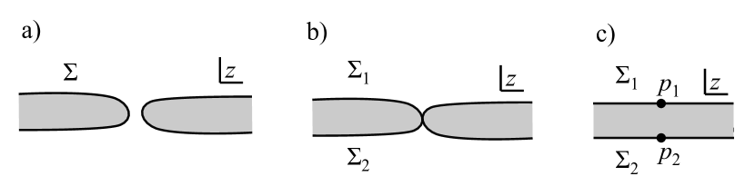
Figure 7: (a) The complement of the shaded region of the complex $z$-plane is a Riemann surface $\Sigma$ with boundary. It consists of an upper and lower half plane connected through a narrow neck. (b) In real codimension 1, the neck collapses and $\Sigma$ degenerates to a pair of branches $\Sigma_{1}$ and $\Sigma_{2}$ glued together along a double point. (c) In this picture, the two branches have been separated. Now $\Sigma_{1}$ and $\Sigma_{2}$ are upper and lower half-planes, respectively, with distinguished boundary punctures $p_{1}$ and $p_{2}$. Gluing $p_{1}$ to $p_{2}$ will return us to the singular configuration in (b).

A trivialization of the real spin bundle ${\mathcal{E}}\to\partial\Sigma$ is given by any nonzero section of ${\mathcal{E}}$. For example, if $\Sigma$ is the upper half $z$ plane, then ${\mathcal{E}}\to\partial\Sigma$ can be trivialized by $\psi=\pm\sqrt{\mathrm{d}z}$, and if $\Sigma$ is the lower half $z$ plane, then ${\mathcal{E}}\to\partial\Sigma$ can be trivialized by $\psi=\pm{\mathrm{i}}\sqrt{\mathrm{d}z}$.

With this in place, we can return to our problem. In fig. 7, we show the same open-string degeneration as in fig. 6, but now we zoom in on the important region where the degeneration occurs and do not specify what the Riemann surface $\Sigma$ looks like outside this region. The open-string degeneration is drawn in the figure ignoring spin structures and their trivializations. In figure 8, we repeat fig. 7(a), but now providing information about the trivializations of spin structures.

First of all, as there are no boundary punctures in this picture, the real spin bundle of $\partial\Sigma$ is supposed to be trivialized everywhere in the picture. The trivializations are easy to describe in the regions – the upper and lower left and right in the figure – in which $\partial\Sigma$ is parallel to the real $z$ axis. We will use the fact that as $\Sigma$ is a region in the complex $z$ plane, the complex 1-form $\mathrm{d}z$ is defined everywhere on $\Sigma$; similarly it is possible to make a global choice of sign of $\psi=\sqrt{\mathrm{d}z}$, though such a $\psi$ will not be everywhere real on $\partial\Sigma$. The overall sign of what we mean by $\sqrt{\mathrm{d}z}$ will not be important in what follows.

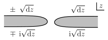
Figure 8: Here we repeat fig. 7(a), but now providing information on the trivialization of the spin bundle of $\partial\Sigma$. On the upper and lower left and right of the figure, $\partial\Sigma$ is parallel to the real $z$ axis and so the spin structure is trivialized by a choice of $\pm\sqrt{z}$ (the upper regions) or $\pm{\mathrm{i}}\sqrt{\mathrm{d}z}$ (the lower regions).

We begin on the upper right of the picture with ${\mathcal{E}}$ trivialized by $\psi=\sqrt{\mathrm{d}z}$. (It would add nothing essentially new to use $-\sqrt{\mathrm{d}z}$ in the starting point, as the overall sign of $\sqrt{\mathrm{d}z}$ is anyway arbitrary.) Now on the upper left of the picture, we pick a trivialization $\pm\sqrt{\mathrm{d}z}$. This sign is meaningful, given that we used the trivialization $+\sqrt{\mathrm{d}z}$ on the upper right. Now we continue through the narrow neck into the lower part of the picture. As we do this, the boundary of $\partial\Sigma$ bends counterclockwise by an angle $\pi$ on the right of the figure and by an angle $-\pi$ on the left. As a result, a section of ${\mathcal{S}}\to\partial\Sigma$ has to acquire a phase in order to remain real. The trivialization of ${\mathcal{E}}$ that is defined as $\sqrt{\mathrm{d}z}$ on the upper right will evolve to ${\mathrm{i}}\sqrt{\mathrm{d}z}$ on the lower right, and the trivialization of ${\mathcal{E}}$ that is defined as $\pm\sqrt{\mathrm{d}z}$ on the upper left will evolve to $\mp{\mathrm{i}}\sqrt{\mathrm{d}z}$ on the lower left.

We see that with one choice of sign on the left part of the picture, the trivializations agree on the upper left and upper right of the figure but not on the lower left and lower right; with the other choice of sign, matters are reversed. So when $\Sigma$ degenerates to the union of two branches $\Sigma_{1}$ and $\Sigma_{2}$ that are to be joined by gluing a point $p_{1}\in\partial\Sigma_{1}$ to a point $p_{2}\in\partial\Sigma_{2}$, as in fig. 7(c), the trivialization of the spin structure of the boundary jumps in crossing $p_{1}$ but not in crossing $p_{2}$ or in crossing $p_{2}$ but not in crossing $p_{1}$. In the construction studied in [3, 4, 5, 6], precisely one of $p_{1}$ and $p_{2}$ plays no role and can be forgotten. This is the basic reason that the boundary of ${\overline{\mathcal{M}}}$ behaves as if it is of real codimension two and the correlation functions are well-defined. We provide more detail momentarily.

3.10 Computations of Disc Amplitudes

Several concrete methods to compute in this framework have been deduced [3, 4, 5, 6]. Here we will just describe the simplest computations of disc amplitudes.

First let us discuss the proper normalization of a disc amplitude. We write $\mathrm{g}_{\mathrm{st}}$ for the string coupling constant in topological gravity of closed Riemann surfaces with its usual normalization, and $\widetilde{\mathrm{g}}_{\mathrm{st}}$ for the string coupling constant in the present theory.

In the standard approach, genus $g$ amplitudes are weighted by a factor of $\mathrm{g}_{\mathrm{st}}^{2g-2}$. With theory ${\mathcal{T}}$ included, this is replaced by $\widetilde{\mathrm{g}}_{\mathrm{st}}^{2g-2}2^{g-1}$, where $2^{g-1}$ is the partition function of theory ${\mathcal{T}}$ (eqn. (3.5)). The relation between the two is thus

$$\widetilde{\mathrm{g}}_{\mathrm{st}}=\frac{\mathrm{g}_{\mathrm{st}}}{\sqrt{2}}.$$ (3.36)

A disc has Euler characteristic 1, so a disc amplitude is weighted by $1/\widetilde{\mathrm{g}}_{\mathrm{st}}=\sqrt{2}/\mathrm{g}_{\mathrm{st}}$. The partition function of theory ${\mathcal{T}}$ on a disc is $1/2$ (as a disc has only one spin structure). However, for any given set of boundary punctures, there are two possible piecewise trivializations of the spin structure of the boundary, with the requisite jumps across boundary punctures. These two choices will contribute equally in the simple computations we will discuss, so we can take them into account by including a factor of 2.

The factors discussed so far combine to $2\cdot\frac{1}{2}\sqrt{2}/\mathrm{g}_{\mathrm{st}}=\sqrt{2}/\mathrm{g}_{\mathrm{st}}$. In addition, in [3] it was found convenient to include a factor of $1/\sqrt{2}$ for every boundary puncture. Thus, let $\Sigma$ be a disc with $m$ boundary punctures and $n$ bulk punctures labeled by integers $d_{1},\dots,d_{n}$; let $\overline{\mathcal{M}}$ be the compactified moduli space of conformal structures on $\Sigma$. Then refining eqn. (3.1), the general disc ampitude is

$$\langle\tau_{d_{1}}\tau_{d_{2}}\dots\tau_{d_{n}}\sigma^{m}\rangle_{D}=\frac{2^{(1-m)/2}}{\mathrm{g}_{\mathrm{st}}}\int_{\overline{\mathcal{M}}}\psi_{1}^{d_{1}}\psi_{2}^{d_{2}}\cdots\psi_{n}^{d_{n}}.$$ (3.37)

This formula agrees with eqn. (18) in [3]. We have included factors of $\mathrm{g}_{\mathrm{st}}$ in this explanation, because that helps determine the factors of 2 that are needed to ensure that the theory is consistent with the standard normalization in the case that a surface $\Sigma$ has no boundary. However, in mathematical treatments, $\mathrm{g}_{\mathrm{st}}$ is often set to 1, and we will do so in the rest of this section. (No topological information is lost, since a given correlation function receives contributions only from surfaces with a given Euler characteristic, and this determines the power of $\mathrm{g}_{\mathrm{st}}$.)

In interpreting eqn. (3.37), we consider the boundary punctures to be inequivalent and labeled, and we sum over all possible cyclic orderings. For example, let us compute $\langle\sigma\sigma\sigma\rangle$, which receives a contribution only from a disc with three boundary punctures labeled 1,2,3. There are two cyclic orderings (namely 123 and 132), and for each cyclic ordering, $\overline{\mathcal{M}}$ is just a point, with $\int_{\overline{\mathcal{M}}}1=1$. So after settting $\mathrm{g}_{\mathrm{st}}=1$, eqn. (3.37) with $n=0$, $m=3$, and including a factor of 2 from the sum over cyclic orderings, gives

$$\langle\sigma^{3}\rangle=1.$$ (3.38)

Getting this formula was the motivation to include a factor $1/\sqrt{2}$ for each boundary puncture. Another simple formula is

$$\langle\tau_{0}\sigma\rangle=1.$$ (3.39)

This is again easy because the moduli space is a point. With boundary punctures only, eqn. (3.38) is the only nonzero amplitude, for dimensional reasons, and similarly (3.39) is the only additional nonzero disc amplitude with insertions of $\sigma$ and $\tau_{0}$ only.

Figure 9: (a) If the two-sphere $\Sigma$ degenerates to two branches with punctures $z_{2}$ and $z_{3}$ on opposite sides, then the 1-form $\rho=\mathrm{d}z/(z-z_{2})(z-z_{3})$ has poles on each branch, so in particular it is nonzero on each branch. (When $\Sigma$ degenerates, $\rho$ also acquires poles at the double point that the two branches have in common, with equal and opposite residues on the two sides.) $\lambda$ also remains nonzero. (b) If instead $z_{2}$ and $z_{3}$ are on the same branch, then all poles of $\rho$ are on that branch and in fact $\rho=0$ on the other branch. Since $\lambda$ is defined by setting $z=z_{1}$ in $\rho$, $\lambda$ vanishes if, as sketched here, $z_{1}$ is on the branch on which $\rho$ is identically zero.

The simplest method to compute arbitrary disc amplitudes is given by the recursion relations in Theorem 1.5 of [3], and indeed the first of these relations is sufficient. To explain it, first we recall the genus 0 recursion relations of [17]. It is convenient to define

$$\langle\langle\tau_{d_{1}}\tau_{d_{2}}\cdots\tau_{d_{s}}\rangle\rangle=\left\langle\tau_{d_{1}}\tau_{d_{2}}\cdots\tau_{d_{s}}\exp\left(\sum_{n=0}^{\infty}t_{n}\tau_{n}\right)\right\rangle.$$ (3.40)

Thus $\langle\langle\tau_{d_{1}}\tau_{d_{2}}\cdots\tau_{d_{s}}\rangle\rangle$ is an amplitude with specified insertions as shown, with all possible additional insertions weighted by powers of the $t_{n}$. We also write $\langle\langle\tau_{d_{1}}\tau_{d_{2}}\cdots\tau_{d_{s}}\rangle\rangle_{0}$ for the genus 0 contribution to $\langle\langle\tau_{d_{1}}\tau_{d_{2}}\cdots\tau_{d_{s}}\rangle\rangle$. Then one has the genus 0 recursion relation

$$\langle\langle\tau_{d_{1}}\tau_{d_{2}}\tau_{d_{3}}\rangle\rangle_{0}=\langle\langle\tau_{d_{1}-1}\tau_{0}\rangle\rangle_{0}\langle\langle\tau_{0}\tau_{d_{2}}\tau_{d_{3}}\rangle\rangle_{0}.$$ (3.41)

The proof goes roughly as follows. For a smooth genus 0 surface $\Sigma$, we take the complex $z$-plane plus a point at infinity. We denote the specified punctures as $z_{1},z_{2},z_{3}$. We will construct a convenient section $\lambda$ of the line bundle ${\mathcal{L}}_{1}\to\overline{\mathcal{M}}$ whose fiber is the cotangent bundle to $\Sigma$ at $z_{1}$. Let $\rho$ be the 1-form

$$\rho=(z_{2}-z_{3})\frac{\mathrm{d}z}{(z-z_{2})(z-z_{3})}.$$ (3.42)

It has poles at $z=z_{2},z_{3}$, with residues 1 and $-1$, and elsewhere is regular and nonzero. These properties characterize $\rho$ uniquely, so $\rho$ does not depend on the coordinates used in writing the formula. Upon setting $z=z_{1}$ in $\rho$, we get a holomorphic section $\lambda$ of ${\mathcal{L}}_{1}\to\overline{\mathcal{M}}$; the divisor $\sf D$ of the zeroes of this section represents $c_{1}({\mathcal{L}}_{1})$. But $\lambda$ never vanishes when $\Sigma$ is smooth, because $\rho$ has no zeroes on the finite $z$-plane or at $z=\infty$. If $\Sigma$ degenerates to two components with $z_{2}$ and $z_{3}$ on opposite sides (fig. 9(a)), $\lambda$ is still everywhere nonzero. But if $z_{2}$ and $z_{3}$ are contained in the same component (fig. 9(b)), then $\lambda$ vanishes on the other component. Finally, then, $\rho$ vanishes precisely if, as in the figure, $z_{1}$ is contained in the opposite component from the one containing $z_{2}$ and $z_{3}$. Moreover, this is a simple zero (because $\rho$ has a simple zero at $z_{2}=z_{3}$). So in $\tau_{d_{1}}=c_{1}({\mathcal{L}}_{1})^{d_{1}}$, we can replace one factor of $c_{1}({\mathcal{L}}_{1})$ with a restriction to the divisor $\sf D$ that is depicted in fig. 9(b). After making this substitution, we are left with an insertion of $\tau_{d_{1}-1}$ on one branch and insertions of $\tau_{d_{2}}$ and $\tau_{d_{3}}$ on the other; in addition, a new puncture corresponding to an insertion of $\tau_{0}$ appears on each branch, where the two branches meet. All this leads to the right hand side of eqn. (3.41). It is not difficult to see that this recursion relation uniquely determines all genus zero amplitudes, modulo the statement that the only nonzero amplitude with insertions of $\tau_{0}$ only is $\langle\tau_{0}^{3}\rangle_{0}=1$.

The disc recursion relation that we aim to describe can be formulated and proved in almost the same way. Similarly to the previous case, we define

$$\langle\langle\tau_{d_{1}}\tau_{d_{2}}\cdots\tau_{d_{s}}\sigma^{m}\rangle\rangle=\left\langle\tau_{d_{1}}\tau_{d_{2}}\cdots\tau_{d_{s}}\sigma^{m}\exp\left(\sum_{n=0}^{\infty}t_{n}\tau_{n}+v\sigma\right)\right\rangle,$$ (3.43)

and write $\langle\langle\tau_{d_{1}}\tau_{d_{2}}\cdots\tau_{d_{s}}\sigma^{m}\rangle\rangle_{D}$ for the disc contribution. The desired recursion relation is

$$\langle\langle\tau_{n}\sigma\rangle\rangle_{D}=\langle\langle\tau_{n-1}\tau_{0}\rangle\rangle_{0}\langle\langle\tau_{0}\sigma\rangle\rangle_{D}+\langle\langle\tau_{n-1}\rangle\rangle_{D}\langle\langle\sigma^{2}\rangle\rangle_{D}.$$ (3.44)

Given a knowledge of eqns. (3.38) and (3.39) and vanishing of $\langle\tau_{0}^{n}\sigma^{m}\rangle_{D}$ for other values of $n,m$, it is not difficult to see that eqn. (3.44) determines all disc amplitudes in terms of the genus 0 amplitudes. These in turn can be determined, for example, from (3.41).

The proof of eqn. (3.44) is rather similar to the proof of the genus zero recursion relation (3.41). However, we will have to explain more fully what is meant in saying that one of the punctures in an open-string degeneration should be forgotten.

Roughly speaking, we are going to again compute $c_{1}({\mathcal{L}}_{1})$, for one of the bulk punctures, from the zeroes of a convenient section $\lambda$ of ${\mathcal{L}}_{1}$. However, here because $\overline{\mathcal{M}}$ has a boundary, we have to discuss how to relate $c_{1}({\mathcal{L}}_{1})$ to the zeroes of a section.

As discussed in section 3.9, the boundary $\partial\overline{\mathcal{M}}$ of $\overline{\mathcal{M}}$ has a forgetful map in which precisely one of the extra boundary punctures that appears at an open-string degeneration is forgotten. Let us write $\overline{\mathcal{N}}$ for the remaining moduli space when this puncture is forgotten, so that the forgetful map is $\pi:\partial\overline{\mathcal{M}}\to\overline{\mathcal{N}}$.

Simplifying a little, the recipe [3] is that $c_{1}({\mathcal{L}}_{1})$ can be represented by the zeros of any section $s$ of ${\mathcal{L}}_{1}$ that is nonvanishing everywhere along $\partial\overline{\mathcal{M}}$, and whose restriction to $\partial\overline{\mathcal{M}}$ is a pullback from $\overline{\mathcal{N}}$. Alternatively, one can still calculate $c_{1}({\mathcal{L}}_{1})$ using any section $s$ of ${\mathcal{L}}_{1}$ that is everywhere nonzero along the boundary, even if its restriction to the boundary is not a pullback. But in this case, $c_{1}({\mathcal{L}}_{1})$ is represented by a sum of two contributions, one involving in the usual way the zeroes of $s$, and the second measuring the failure of the restriction of $s$ to be a pullback.

Setting $z=x+{\mathrm{i}}y$, we take a smooth disc $D$ to be the closed upper half-plane $y\geq 0$ plus a point at infinity. On the left hand side of eqn. (3.44), we see a distinguished bulk puncture that we place at $z_{1}=x_{1}+{\mathrm{i}}y_{1}$, $y_{1}>0$, and a distinguished boundary puncture that we place at $x_{0}$. In the present case, there is a convenient section $\lambda$ of ${\mathcal{L}}_{1}$ that is everywhere nonzero along the boundary, but whose restriction to the boundary is not a pullback. To construct it, rather as before, we set

$$\rho=(\overline{z}_{1}-x_{0})\frac{\mathrm{d}z}{(z-\overline{z}_{1})(z-x_{0})}.$$ (3.45)

This 1-form is regular and nonzero throughout $D$, except at the boundary point $x_{0}$. Evaluating $\rho$ at $z=z_{1}$, we get a section $\lambda$ of ${\mathcal{L}}_{1}$ that is regular and nonzero as long as $D$ is smooth.

Figure 10: (a) A disc $D$ splits up into the union of a disc and a sphere (upper half of the drawing). If the bulk puncture $z_{1}$ is contained in the sphere, then the section $\lambda$ vanishes. To see this, take the closed oriented double cover, obtained here by adding additional components (lower half of the drawing, sketched with dotted lines). It is a union of three spheres connected at double points. The differential $\rho$ has poles only on the bottom two components and vanishes identically on the top component. So, setting $z=z_{1}$ to define $\lambda$, we learn that, with $z_{1}$ being in the top component, $\lambda$ vanishes. (b) The same disc $D$ splits into a union of two discs, again comprising the upper half of the drawing. The interesting case is that $z_{1}$ and $x_{0}$ are on opposite sides, as shown. The oriented double cover (the full drawing including the bottom half) is a union of two spheres. $\rho$ has poles at $x_{0}$ and $\overline{z}_{1}$ and so is nonzero on both branches; hence $\lambda\not=0$ along this divisor. On the branch containing $z_{1}$, $\rho$ has an additional pole at the point labeled $p_{1}$ where the two branches meet. Therefore $\lambda$ depends on $p_{1}$, and, if $p_{1}$ is the boundary puncture that is forgotten by the forgetful map $\pi:\partial\overline{\mathcal{M}}\to\overline{\mathcal{N}}$, then along this component of the boundary, $\lambda$ is not a pullback.

At a closed-string degeneration, where $D$ splits up into the union of a two-sphere and a disc (fig. 10(a)), $\lambda$ has a simple zero if and only if $z_{1}$ is on the two-sphere component. This is responsible for the first term on the right hand side of the recursion relation (3.44). At an open-string degeneration, where $D$ splits up into the union of two discs (fig. 10(b)), $\lambda$ remains everywhere nonzero. However, in case the boundary puncture that is supposed to be forgotten is in the same component as $z_{1}$, $\lambda$ restricted to $\partial\overline{{\mathcal{M}}}$ is not a pullback from $\overline{\mathcal{N}}$. The second term on the right hand side of eqn. (3.44) corrects for this failure. See fig. 10 for an explanation of the statements about the behavior of $\lambda$ at degenerations.

4 Interpretation Via Matrix Models

4.1 The Loop Equations

Let us now briefly recapitulate the representation of topological gravity in terms of random matrix models. The simplest models are single matrix models of the form

$$Z=\frac{1}{{\rm vol}(U(N))}\int\mathrm{d}\Phi\cdot\exp\left(-\frac{1}{\mathrm{g}_{\mathrm{st}}}{\rm Tr}\,W(\Phi)\right)$$ (4.1)

Here $\Phi$ is a hermitian $N\times N$ matrix integrated with the Euclidean measure for each matrix element, $W(x)$ is a complex polynomial, say of degree $d+1$, and $\mathrm{g}_{\mathrm{st}}$ is the string coupling constant. Since we divide by the volume of the “gauge group” $U(N)$, this integral should be considered the zero-dimensional analogue of a gauge theory—we integrate over matrices $\Phi$ modulo gauge transformations

$$\Phi\to U\cdot\Phi\cdot U^{-1}.$$ (4.2)

In general, if $\mathrm{Re}\,W$ is not bounded below, one needs to complexify the matrix $\Phi$ and pick a suitable integration contour in the space of complex matrices to make the integral well-defined. For a formal expansion in powers of $\mathrm{g}_{\mathrm{st}}$ and even for the formal expansion in powers of $1/N$ that we will make shortly, this is not necessary and we can consider (4.1) as a formal expression.

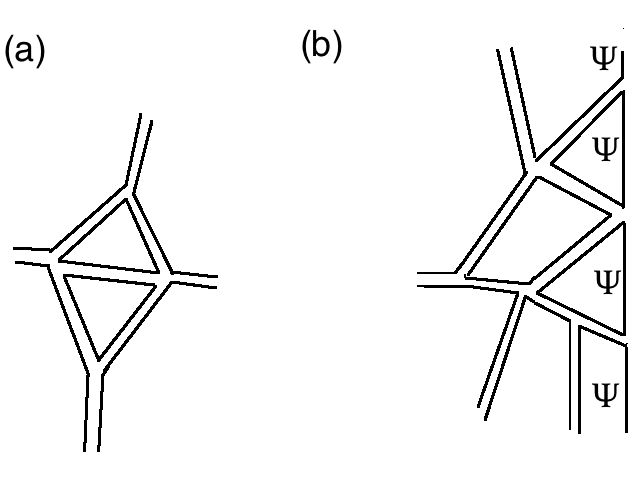
Figure 11: (a) Feynman diagrams of the matrix model are naturally ribbon graphs. The two sides of a ribbon represent the flow of the two “indices” of an $N\times N$ matrix $M^{i}{}_{j}$, $i,j=1,\dots,N$. The edges of the ribbons form closed loops. Gluing a disc to each such loop, the union of the ribbons and the discs is a two-manifold $\Sigma$ without boundary on which the given Feynman diagram can be drawn. (The edges of the ribbon are oriented – not shown here – because the two indices transform according to inequivalent, dual representations of $U(N)$. As a result, $\Sigma$ has a natural orientation. (A similar model with symmetry group $O(N)$ or $Sp(N)$ leads to unoriented two-manifolds.) (b) New variables $\Psi,$ $\overline{\Psi}$ transforming in the $N$-dimensional representation of $U(N)$ and its dual are added to the matrix model. Because $\Psi^{i}$ and $\overline{\Psi}_{j}$, $i,j=1,\dots,N$ carry only a single “index” – rather than the two indices of the matrix $M^{i}{}_{j}$ – their propagator is naturally represented by a single line rather than the double line of the matrix propagator. These single lines provide boundaries of the surface $\Sigma$, so now we get a ribbon graph on $\Sigma$ with $\Psi$ propagating on the boundary of $\Sigma$, as shown. For the model described in the text, the $\Psi$ propagtor is $1/z$ and this gives a factor $1/z^{L}$ where $L$ is the length of the boundary.

In a perturbative expansion near a critical point of $W(\Phi)$, the Feynman diagrams become so-called “fat” or ribbon graphs that can be conveniently represented (see fig. 11(a)) by a double line [57]. These are graphs, in general with $\ell$ loops, that can be naturally drawn on some oriented two-manifold of genus $g$. The contribution of such a graph to the expansion of the matrix integral is weighted by a factor

$$(\mathrm{g}_{\mathrm{st}}N)^{\ell}\mathrm{g}_{\mathrm{st}}^{2g-2}.$$ (4.3)

The large $N$ or ’t Hooft limit is obtained by taking the rank $N$ of the matrix to infinity and simultaneously the coupling $\mathrm{g}_{\mathrm{st}}$ to zero, keeping fixed the combination

$$\mu=\mathrm{g}_{\mathrm{st}}N.$$ (4.4)

In the limit, all graphs with a fixed genus and an arbitrary number of holes contribute in the same order, so the matrix integral has an asymptotic expansion of the form

$$Z\sim\exp\left(\sum_{g\geq 0}{\mathrm{g}_{\mathrm{st}}}^{2g-2}{\cal F}_{g}\right),$$ (4.5)

where ${\cal F}_{g}$ is the contribution of ribbon graphs of genus $g$. In general, the matrix integral depends on the coefficients of the potential $W$ and the particular critical point around which the expansion is made. We describe the critical points at the end of this section.

Matrix integrals are governed by Virasoro constraints that are associated to the vector fields $L_{n}\sim-{\rm Tr}\,\Phi^{n+1}\frac{\partial}{\partial\Phi}$. Though these constraints can be deduced directly from that representation of $L_{n}$, a fuller understanding with details that we will need below can be obtained by diagonalizing the matrix as $\Phi=U\Lambda U^{-1}$, with $U$ unitary and $\Lambda=\mathrm{diag}(\lambda_{1},\lambda_{2},\cdots,\lambda_{N})$. The integral over $U$ cancels the factor of $1/\mathrm{vol}(U(N))$ in the definition of the matrix integral, and the integral becomes

$$Z=\int\mathrm{d}^{N}\!\lambda\prod_{I<J}\left(\lambda_{I}-\lambda_{J}\right)^{2}\exp\left(-\sum_{I}\frac{1}{\mathrm{g}_{\mathrm{st}}}W(\lambda_{I})\right).$$ (4.6)

If $x_{i},\,i=1,\dots,d$ are the critical points of the polynomial $W(x)$, then the critical points of the matrix function ${\rm Tr}\,W(\Phi)$ are found by setting each $\lambda_{I}$ equal to one of the $x_{i}$. A critical point is labeled by the number $N_{i}$ of eigenvalues with $\lambda_{I}=x_{i}$. (Note that the eigenvalues $\lambda_{I}$ are only defined up to permutation.) The large $N$ limit is taken is such a way that the “filling fractions”

$$\mu_{i}=\mathrm{g}_{\mathrm{st}}N_{i},\qquad i=1,\ldots,d,$$ (4.7)

are all kept finite. These parameters characterize the saddle-points, and together with the coefficients of the polynomial $W(x)$ play the role of moduli of the matrix model. (In our application, because it only involves a local portion of the spectral curve, we will not really see these parameters.)

To derive the Virasoro constraints on the matrix integral, one can start with

$$0=\int\mathrm{d}^{N}\!\lambda\sum_{K}\frac{\partial}{\partial\lambda_{K}}\left(\frac{1}{x-\lambda_{K}}\prod_{I<J}\left(\lambda_{I}-\lambda_{J}\right)^{2}\exp\left(-\sum_{I}\frac{1}{\mathrm{g}_{\mathrm{st}}}W(\lambda_{I})\right)\right).$$ (4.8)

This implies the identity

$$\left\langle\left(\sum_{K}\frac{1}{x-\lambda_{K}}\right)^{2}-\frac{1}{\mathrm{g}_{\mathrm{st}}}\sum_{K}\frac{W^{\prime}(\lambda_{K})}{x-\lambda_{K}}\right\rangle=0,$$ (4.9)

where the symbol $\langle\cdots\rangle$ is defined by

$$\langle A\rangle=\frac{1}{Z}\int\mathrm{d}^{N}\!\lambda\,A\,\prod_{I<J}\left(\lambda_{I}-\lambda_{J}\right)^{2}\exp\left(-\sum_{I}\frac{1}{\mathrm{g}_{\mathrm{st}}}W(\lambda_{I})\right).$$ (4.10)

In eqn. (4.9) we see the matrix resolvent ${\rm Tr}\,(x-\Phi)^{-1}=\sum_{K}\/(x-\lambda_{K})^{-1}$, but as we will see a slightly more convenient variable is

$$J(x)=\frac{1}{2}W^{\prime}(x)-{\mathrm{g}_{\mathrm{st}}}{\rm Tr}\frac{1}{x-\Phi}=\frac{1}{2}W^{\prime}(x)-{\mathrm{g}_{\mathrm{st}}}\sum_{K}\frac{1}{x-\lambda_{K}}.$$ (4.11)

The identity (4.9) is equivalent to

$$\langle J(x)^{2}\rangle=\left\langle\frac{1}{4}W^{\prime}(x)^{2}-\mathrm{g}_{\mathrm{st}}\sum_{K}\frac{W^{\prime}(x)-W^{\prime}(\lambda_{K})}{x-\lambda_{K}}\right\rangle,$$ (4.12)

and we note that if $W$ is a polynomial, then

$$f(x)=-\mathrm{g}_{\mathrm{st}}\left\langle\sum_{K}\frac{W^{\prime}(x)-W^{\prime}(\lambda_{K})}{x-\lambda_{K}}\right\rangle$$ (4.13)

is a polynomial in $x$, as is

$$P(x)=\frac{1}{4}W^{\prime}(x)^{2}+f(x).$$ (4.14)

If $W$ is a general function $W=\sum_{n\geq 0}u_{n}x^{n}$ regular at $x=0$, then $P(x)$ is no longer a polynomial but is regular at $x=0$.

When we insert the expression $J(x)$ inside the matrix integral (4.6), where we now consider a general function

$$W(x)=\sum_{n\geq 0}u_{n}x^{n},$$ (4.15)

it can be written as a differential operator

$$J(x)=\frac{1}{2}\sum_{n\geq 0}\left\{(n+1)u_{n+1}x^{n}+2\mathrm{g}_{\mathrm{st}}^{2}\frac{\partial}{\partial u_{n}}x^{-n-1}\right\}.$$ (4.16)

Comparing to standard formulas in conformal field theory, we are led to set

$$J(x)=\frac{\mathrm{g}_{\mathrm{st}}}{\sqrt{2}}\partial\varphi(x)$$ (4.17)

where $\varphi(x)$ is a chiral boson in a $c=1$ conformal field theory with canonical two-point function $\partial\varphi(x)\partial\varphi(y)\sim 1/(x-y)^{2}$. Thus

$$\partial\varphi(x)={\sqrt{2}}\left(\frac{W^{\prime}(x)}{2\mathrm{g}_{\mathrm{st}}}-\sum_{K}\frac{1}{x-\lambda_{K}}\right),$$ (4.18)

and formally

$$\varphi(x)=\sqrt{2}\left(\frac{W(x)}{2\mathrm{g}_{\mathrm{st}}}-\sum_{K}\log(x-\lambda_{K})\right)=\sqrt{2}\left(\frac{W(x)}{2\mathrm{g}_{\mathrm{st}}}-\log\det(x-\Phi)\right).$$ (4.19)

The corresponding stress tensor is

$$T(x)=\frac{1}{2}(\partial\varphi)^{2}=\frac{1}{\mathrm{g}_{\mathrm{st}}^{2}}J(x)^{2}.$$ (4.20)

Making the standard mode expansion

$$T(x)=\sum_{k\in{\mathbb{Z}}}\frac{L_{k}}{x^{k+2}},$$ (4.21)

the equation (4.12) becomes a set of differential equations for the partition function,

$$\sum_{k\in{\mathbb{Z}}}\frac{L_{k}}{x^{k+2}}Z=\mathrm{g}_{\mathrm{st}}^{2}P(x)Z.$$ (4.22)

Since $P(x)$ is regular at $x=0$, it contributes only to the terms in eqn. (4.22) with $k\leq-2$ and those terms serve to determine $P(x)$. However, for $k\geq-1$, $P(x)$ does not contribute to eqn. (4.22) and we get differential equations satisfied by $Z$:

$$L_{n}Z=0,~{}~{}~{}n\geq-1.$$ (4.23)

In this range of $n$, the $L_{n}$ are

$$L_{-1} = \sum_{k\geq 1}ku_{k}\frac{\partial}{\partial u_{k-1}},$$ (4.24)

$$L_{n} = \sum_{k}ku_{k}\frac{\partial}{\partial u_{k+n}}+\mathrm{g}_{\mathrm{st}}^{2}\sum_{i+j=n}\frac{\partial^{2}}{\partial u_{i}\partial u_{j}},\qquad n\geq 0.$$ (4.25)

So far, all of this is true for any $N$; we have not made any large $N$ approximation. For any function $h$, the quantity $\langle\mathrm{g}_{\mathrm{st}}{\rm Tr}\,h(\Phi)\rangle$ has a limit for large $N$, and for any two functions $h_{1},h_{2}$, one has a large $N$ factorization

$$\langle\mathrm{g}_{\mathrm{st}}^{2}{\rm Tr}\,h_{1}(\Phi)\,{\rm Tr}\,h_{2}(\Phi)\rangle\overset{N\to\infty}{\longrightarrow}\langle\mathrm{g}_{\mathrm{st}}{\rm Tr}\,h_{1}(\Phi)\rangle\langle\mathrm{g}_{\mathrm{st}}{\rm Tr}\,h_{2}(\Phi)\rangle.$$ (4.26)

These properties can be demonstrated by an elementary study of the matrix integral. In particular, both $\langle J\rangle$ and $f(x)$ have large $N$ limits, and in the large $N$ limit

$$\langle J(x)^{2}\rangle=\langle J(x)\rangle^{2}.$$ (4.27)

We define

$$y=\langle J(x)\rangle_{0},$$ (4.28)

where the subscript denotes the the large $N$ limit. Eqn. (4.12) becomes for large $N$ a hyperelliptic equation for $y$

$$y^{2}=P(x)=\frac{1}{4}W^{\prime}(x)^{2}+f(x)$$ (4.29)

and defines what is known as the spectral curve ${\mathcal{C}}$. In eqn. (4.29), $y$, $W$, and $f$ all depend on the “coupling parameters” $u_{i}$, though this is not shown explicitly. Remarkably, the spectral curve fully captures the solution of the matrix model. That is, all the perturbative functions ${\cal F}_{g}$ can be completely calculated using the geometric data of the spectral curve [58].

Suppose that $W$ is a polynomial of degree $d+1$, thus with $d$ critical points $p_{1},\dots,p_{d}$. Concretely, when one takes the large $N$ limit of the matrix integral, the first step is to pick a critical point of the matrix function ${\rm Tr}\,W(\Phi)=\sum_{K=1}^{N}W(\lambda_{K})$ about which to expand. The critcal points of this matrix function are found simply by setting each of the $\lambda_{K}$ equal to one of the $p_{j}$. Up to a permutation of the $\lambda$’s, the critical points are classified by the number $N_{i}$ of eigenvalues that equal $p_{i}$. The $N_{i}$ are subject to one constraint

$$\sum_{i=1}^{d+1}N_{i}=N.$$ (4.30)

A large $N$ limit is obtained in general by taking $N\to\infty$ keeping fixed

$$\mu_{i}=\mathrm{g}_{\mathrm{st}}N_{i}.$$ (4.31)

In the large $N$ limit, the $\mu_{i}$ behave as continuous variables constrained only by

$$\sum_{i}\mu_{i}=\mu.$$ (4.32)

Thus if $W$ is of degree $d+1$, there are $d$ “moduli” $\mu_{i}$ that appear in constructing the large $N$ limit. We note from eqn. (4.13) that $f(x)$ is a polynomial of degree $d-1$ in $x$ and so has $d$ coefficients. These $d$ coefficients are functions of the moduli $\mu_{i}$ of the matrix model. So except for constraints coming from keeping the $N_{i}$ real and positive, a $d-1$-parameter family of $f$’s can arise, even for fixed $W$, by varying the critical point about which one expands the matrix model.

In the above derivation, for finite $N$, we discovered that the matrix integral is governed by an operator-valued conformal field $\partial\varphi(x)$. For finite $N$, this field depends on the parameters of the matrix model, namely the $u_{i}$ and $N$, as well as $x$. In the large $N$ limit, the matrix integral can be defined by an expansion around a particular saddle point, and then new parameters appear. For the “bare” matrix integral, without trying to compute the expectation value of the resolvent, the extra parameters are the $\mu_{i}$. When one tries to compute the expectation value of the resolvent, there is an additional binary choice, since $\langle J(x)\rangle$ is governed by a quadratic equation with two roots. In the large $N$ limit, and also in the more refined double scaling limit in which $N\to\infty$ with $\mu=\mathrm{g}_{\mathrm{st}}N$ fixed, the formalism with the conformal field $\partial\varphi$ remains valid, but this field now depends on additional parameters – the $\mu_{i}$ and the choice of sign of $\langle J(x)\rangle$.

In our application, the $\mu_{i}$ will not be very important, since we will consider only the local behavior near a particular branch point. However, the extension of the conformal formalism to include the choice of sign of $\langle J(x)\rangle$ is important. It means that $\partial\phi$ should be interpreted as a conformal field on the spectral curve ${\mathcal{C}}$, the double cover of the $x$-plane that is defined by the hyperelliptic equation (4.29). The hyperelliptic curve has an involution $y\to-y$ that exchanges the two choices of the sign of $\langle J(x)\rangle$. Since $\partial\varphi$ is defined as a multiple of $J(x)$ (eqn. (4.17)), $\partial\varphi$ is odd under the hyperelliptic involution.

4.2 Double-Scaling Limits And Topological Gravity

Topological gravity and other models of two-dimensional gravity coupled to matter are obtained by taking a suitable double-scaling limit of the generic matrix model. These scaling limits are best understood in terms of the underlying spectral curve. For the so-called $(2,2p-1)$ minimal model CFT coupled to gravity, the corresponding spectral curve takes the form

$$y^{2}\sim x^{2p-1}.$$ (4.33)

This limiting curve can be obtained by starting from the generic case $y^{2}=P(x)$, where $P$ is a polynomial of degree $2p$, and then making $2p-1$ branch points coincide and sending the remaining one to infinity. In particular for topological gravity, which corresponds to the case $p=1$, we choose to write the underlying curve as

$$\frac{1}{2}y^{2}=x$$ (4.34)

This curve can be obtained, for example, from the simple Gaussian matrix model, with a quadratic polynomial $W(x)=x^{2}$. In this example, the polynomial $P$ is $P(x)=x^{2}-c$, with a constant $c$. There are branch points at $x=\pm\sqrt{c}$. After shifting $x$ by a constant and “zooming in” to a single branch point, one gets the curve of eqn. (4.34).

In the limit that the spectral curve ${\mathcal{C}}$ is described by eqn. (4.34), the operator-valued conformal field $\partial\varphi$ takes a simple form. Because it is odd under the hyperelliptic involution $y\to-y$, its expansion in powers of $x$ has only half-integer powers. We will choose to parametrize the expansion as

$$\frac{1}{2}\mathrm{g}_{\mathrm{st}}\partial\varphi(x)=x^{\frac{1}{2}}-\sum_{n\geq 0}(n+\frac{1}{2})s_{n}x^{n-\frac{1}{2}}-\frac{1}{4}\mathrm{g}_{\mathrm{st}}^{2}\sum_{n\geq 0}\frac{\partial}{\partial s_{n}}x^{-n-\frac{3}{2}}$$ (4.35)

Here $\varphi$ is what would usually be called a twisted chiral boson on the complex $x$-plane, with a twist field at $x=0$ (and another at $x=\infty$). The $s_{n}$ are functions of the parameters $u_{n}$ of an underlying matrix model; the precise relationship depends upon exactly what matrix model one starts with before passing to the limit in which the spectral curve ${\mathcal{C}}$ reduces to the curve $y^{2}=2x$. This relationship is not very important for us.

What is important is the relationship between the $s_{n}$ and the corresponding parameters $t_{n}$ of topological gravity – the parameters that were introduced in eqn. (3.3). This relationship turns out to be

$$t_{n}=\frac{(2n+1)!!}{2^{n}}s_{n}.$$ (4.36)

This statement is part of the relationship between the matrix model and intersection theory on ${\mathcal{M}}_{g,n}$, as proved in [20] as well as[2, 21, 22]. (Note that the factor $2^{n}$, which is not entirely standard, is a consequence of our particular normalization of the spectral curve in eqn. (4.34).)

Inserting these expressions into the loop equations then gives the familiar Virasoro constraints

$$L_{n}Z=0,\qquad n\geq-1,$$ (4.37)

where the operators $L_{n}$ are modes of the stress tensor $T=\frac{1}{2}(\partial\varphi)^{2}$, with $\partial\varphi$ now given by eqn. (4.35). That is, we have

$$L_{-1} = -\frac{\partial}{\partial s_{0}}+\sum_{k\geq 1}(k+\frac{1}{2})s_{k}\frac{\partial}{\partial s_{k-1}}+\frac{1}{2\mathrm{g}_{\mathrm{st}}^{2}}s_{0}^{2},$$ (4.38)

$$L_{0} = -\frac{\partial}{\partial s_{1}}+\sum_{k\geq 0}(k+\frac{1}{2})s_{k}\frac{\partial}{\partial s_{k}}+\frac{1}{16},$$ (4.39)

$$L_{n} = -\frac{\partial}{\partial s_{n+1}}+\sum_{k\geq 0}(k+\frac{1}{2})s_{k}\frac{\partial}{\partial s_{k+n}}+\frac{1}{8}\mathrm{g}_{\mathrm{st}}^{2}\sum_{i+j=n-1}\frac{\partial^{2}}{\partial s_{i}\partial s_{j}},\qquad n\geq 1.$$ (4.40)

Note that these equations fix the normalization of the partition function. In particular if we set all variables $s_{n}=0$ for $n>0$, the $L_{-1}$ constraint gives the genus zero contribution (using $s_{0}=t_{0}$)

$$\frac{\partial}{\partial t_{0}}F_{0}=\frac{1}{2}{t_{0}^{2}}$$ (4.41)

corresponding to three closed-string punctures on the sphere

$$\langle\tau_{0}^{3}\rangle_{0}=1.$$ (4.42)

Note that in that case, with only $t_{0}$ non-zero, the spectral curve becomes

$$\frac{1}{2}y^{2}=x-t_{0}.$$ (4.43)

Returning to a theme from section 2.4, we are now also in a position to write the spectral curve that corresponds to the model computing the volumes of the moduli space of curves. As we have seen in equation (2.24), in that case the values of the coupling constants are

$$t_{n}=\frac{(-1)^{n}\xi^{n-1}}{(n-1)!},\qquad n\geq 2,$$ (4.44)

which corresponds to

$$s_{n}=\frac{n(-1)^{n}2^{2n}\xi^{n-1}}{(2n+1)!},\qquad n\geq 2.$$ (4.45)

Plugging this into (4.35) we find

$$y=\frac{\sin(2\sqrt{\xi x})}{2\sqrt{2\xi}}$$ (4.46)

which is, up to normalization coventions, the known expression for the spectral curve [42].

Perhaps we should add another word about eqn. (4.35). Because the modes of $\partial\varphi(x)$ proportional to $x^{n-1/2}$, $n\geq 0$, commute, we can just declare them to be multiplication by commuting variables $s_{n}$. In a derivation that starts with a matrix model based on a function $W(x)=\sum u_{n}x^{n}$, the $s$’s would be complicated functions of the $u$’s; the precise functions would depend on exactly how one zooms in on a critical point to get to the spectral curve $y^{2}=2x$. Once the coefficients of $x^{n-1/2}$, $n\geq 0$ are fixed as $s_{n}$, the coefficients of other terms in $\partial\varphi(x)$ are uniquely determined by the commutation relations and operator product expansion satisfied by $\partial\varphi(x)$.

4.3 Branes And Open Strings

Before we consider open strings within topological gravity, let us first discuss the formulation of open strings in a general random matrix model. Open strings are naturally included by adding vector degrees of freedom. Let $\Psi,\overline{\Psi}$ be a pair of conjugate $U(N)$ vectors. We can choose these to be bosonic or fermionic variables. The natural interaction with the matrix variable $\Phi$ takes the form

$$\int d\Psi\,d\overline{\Psi}\cdot\exp\left\{-z\overline{\Psi}^{T}\Psi+\overline{\Psi}^{T}\cdot\Phi\cdot\Psi\right\}$$ (4.47)

The effect of adding these additional variables is that now the ribbon graph is naturally drawn on a two-manifold $\Sigma$ with boundary (fig. 11(b)). The propagator of the vector variables has a factor $1/z$, leading to a factor $1/z^{L}$, where $L$ is the length of the boundary of $\Sigma$.

The integral over $\Psi$ and $\overline{\Psi}$ just gives a determinant

$$\det(z-\Phi)^{\pm 1}$$ (4.48)

(apart from an irrelevant constant factor that could be absorbed in normalizing the measure). Here the sign in the exponent is $-1$ or $+1$ if $\Psi,\overline{\Psi}$ are bosons or fermions. In terms of the Feynman diagram expansion, this sign means that for fermions, one will get an extra $-1$ for every component of the boundary of $\Sigma$.

Instead of including the variables $\Psi,$ $\overline{\Psi}$ in the model, it is equivalent to simply consider a matrix model with an extra factor of $\det(z-\Phi)^{\pm 1}$ in the integrand. However, it turns out that it is slightly more convenient to accompany this factor with a prefactor $e^{\mp W(z)/2\mathrm{g}_{\mathrm{st}}}$, which is a “trivial” modification in the sense that it does not depend on the matrix variables. Thus we consider the modified matrix model based on the integral

$$\frac{1}{{\rm vol}(U(N))}\int d\Phi\cdot\exp\left(-\frac{1}{\mathrm{g}_{\mathrm{st}}}{\rm Tr}\,W(\Phi)\right)\det(z-\Phi)^{\pm 1}e^{\mp W(z)/2\mathrm{g}_{\mathrm{st}}}$$ (4.49)

Loosely

$$V(z)=\det(z-\Phi)e^{-W(z)/2\mathrm{g}_{\mathrm{st}}},~{}~{}~{}~{}V^{*}(z)=\det(z-\Phi)^{-1}e^{W(z)/2\mathrm{g}_{\mathrm{st}}}$$ (4.50)

are “operators” that create a brane or antibrane with the “modulus” $z$. We will see that $z$ has the interpretation of a value of $x$, which parametrizes the base of the hyperelliptic spectral curve $y^{2}=P(x)$. More generally, one could add several sets of vector degrees of freedom $\Psi_{a},$ $\overline{\Psi}_{a}$, $a=1,\dots,r$, each with its own modulus $z_{a}$. For definiteness, we will consider the case of insertion of just one factor of $V$:

$$Z_{V}(z)=\frac{1}{{\rm vol}(U(N))}\int d\Phi\cdot\exp\left(-\frac{1}{\mathrm{g}_{\mathrm{st}}}{\rm Tr}\,W(\Phi)\right)\det(z-\Phi)e^{-W(z)/2\mathrm{g}_{\mathrm{st}}}.$$ (4.51)

It is not difficult to derive the modification of the Virasoro equations that reflects the presence of a brane. Repeating the derivation of eqn. (4.9), we get

$$\left\langle\left(\sum_{K}\frac{1}{x-\lambda_{K}}\right)^{2}-\frac{1}{\mathrm{g}_{\mathrm{st}}}\sum_{K}\frac{W^{\prime}(\lambda_{K})}{x-\lambda_{K}}-\sum_{K}\frac{1}{(x-\lambda_{K})(z-\lambda_{K})}\right\rangle_{{V(z)}}=0.$$ (4.52)

Here $\langle A\rangle_{V(z)}$ is defined, by analogy with eqn. (4.10), as the expectation of $A$ in the matrix integral $Z_{V(z)}$. However, it turns out that it is slightly more convenient to make the insertion of $V$ explicit and to write the equivalent identity

$$\left\langle\left(\left(\sum_{K}\frac{1}{x-\lambda_{K}}\right)^{2}-\frac{1}{\mathrm{g}_{\mathrm{st}}}\sum_{K}\frac{W^{\prime}(\lambda_{K})}{x-\lambda_{K}}-\sum_{K}\frac{1}{(x-\lambda_{K})(z-\lambda_{K})}\right)\cdot V(z)\right\rangle=0,$$ (4.53)

where $\langle A\rangle$ is defined precisely as in eqn. (4.10), with the original matrix integral $Z$.

We can write the integral (4.51) as

$$Z_{V}=\frac{1}{{\rm vol}(U(N))}\int d\Phi\cdot\exp\left(-\frac{1}{\mathrm{g}_{\mathrm{st}}}{\rm Tr}\,\left(W(\Phi)-\mathrm{g}_{\mathrm{st}}\log(z-\Phi)\right)\right)e^{-W(z)/2\mathrm{g}_{\mathrm{st}}},$$ (4.54)

suggesting that in the definition of $J(x)$, we should just shift $W(\Phi)\to W(\Phi)-\mathrm{g}_{\mathrm{st}}\log(z-\Phi)$ and hence $W^{\prime}(x)\to W^{\prime}(x)+\mathrm{g}_{\mathrm{st}}/(z-x)$. So we define

$$J(x)=\frac{1}{2}W^{\prime}(x)+\frac{\mathrm{g}_{\mathrm{st}}}{2(z-x)}-{\mathrm{g}_{\mathrm{st}}}\sum_{K}\frac{1}{x-\lambda_{K}}$$ (4.55)

and again

$$T(x)=\frac{J(x)^{2}}{\mathrm{g}_{\mathrm{st}}^{2}}.$$ (4.56)

Because we multiplied the partition function with the factor $e^{-W(z)/2\mathrm{g}_{\mathrm{st}}}$, which introduces an extra explicit dependence on the coefficients $u_{n}$, the formula for $J(x)$ as a differential operator is still given by equation (4.16). We get the identity

$$\left\langle T(x)V(z)\right\rangle=\left(P(x)+\frac{1}{4}\frac{1}{(x-z)^{2}}+\frac{1}{x-z}\frac{\partial}{\partial z}\right)\left\langle V(z)\right\rangle$$ (4.57)

where now

$$P(x)=\frac{1}{4}W^{\prime}(x)^{2}+f(x)-\frac{1}{2}\mathrm{g}_{\mathrm{st}}\frac{W^{\prime}(z)-W^{\prime}(x)}{z-x}.$$ (4.58)

and the definition of $f(x)$ becomes

$$f(x)=-\mathrm{g}_{\mathrm{st}}\frac{1}{\left\langle V(z)\right\rangle}\left\langle\sum_{K}\frac{W^{\prime}(x)-W^{\prime}(\lambda_{K})}{x-\lambda_{K}}\cdot V(z)\right\rangle.$$ (4.59)

$P(x)$ has the same essential properties as before: it is a polynomial of degree $2d$ if $W(x)$ is a polynomial of degree $d+1$, and if $W(x)$ has a general expansion $\sum_{n\geq 0}u_{n}x^{n}$, then $P(x)$ is regular at $x=0$. Moreover, $P(x)$ is regular at $x=z$.

Eqn.  (4.57) has a nice interpretation. We can interpret $V(z)$ as an insertion on the spectral curve (which generically is locally parametrized by $x$) of a primary field of conformal dimension $h=1/4$. On the right hand side of eqn. (4.57), we see the expected singular contributions to the $T(x)V(z)$ operator product expansion,

$$T(x)\cdot V(z)\sim\frac{h}{(x-z)^{2}}V(z)+\frac{1}{x-z}\partial_{z}V(z)+\ldots$$ (4.60)

as well as regular terms that are contained in $P(x)$. Indeed, comparing eqn. (4.19) to the definition (4.50), we see that we can identify $V$ and $V^{*}$ in terms of the conformal field $\varphi$ as

$$V(z)=e^{-\varphi(z)/\sqrt{2}},\qquad V^{*}(z)=e^{\varphi(z)/\sqrt{2}}$$ (4.61)

These are indeed standard expressions for conformal primaries of dimension $1/4$. In the large $N$ limit the scalar $\varphi$ and therefore also the vertex operator $V$ can be expressed in terms of the spectral curve data

$$\varphi(z)\sim\frac{\sqrt{2}}{\mathrm{g}_{\mathrm{st}}}\left(\int^{z}y(x)\mathrm{d}x+{\cal O}(\mathrm{g}_{\mathrm{st}})\right)$$ (4.62)

Since there are two roots in the hyperelliptic spectral curve, there are two saddle-points that dominate the expectation value of $V(z)$

$$\left\langle V(z)\right\rangle\sim\left\{Ae^{-\frac{1}{\mathrm{g}_{\mathrm{st}}}\int^{z}\!y(x)dx}+Be^{\frac{1}{\mathrm{g}_{\mathrm{st}}}\int^{z}\!y(x)dx}\right\}\left(1+{\cal O}(\mathrm{g}_{\mathrm{st}})\right)$$ (4.63)

for some coefficients $A,B$ given by the one-loop correction. These two contributions, that only appear in string perturbation theory, can be considered as the manifestation of the two branes ${\cal B}^{\prime}$ and ${\cal B}^{\prime\prime}$ as discussed in the A-model in section 4.3. Note that they are interchanged by flipping the sign of $\mathrm{g}_{\mathrm{st}}$.

Just as before, the terms in eqn. (4.57) involving negative powers of $x$ give Virasoro constraints

$$L_{n}Z_{V}=0,\qquad n\geq-1,$$ (4.64)

while the terms involving nonnegative powers determine $P(x)$ or are trivial identities. However, there are additional terms in the Virasoro generators. We write the Virasoro generators as $L_{n}=L_{n}^{\sf c}+L_{n}^{o}$, where superscripts ${\sf c}$ and ${\sf o}$ represent “closed-string” and “open-string” contributions. $L_{n}^{\sf c}$ comes from $T(x)$ on the left hand side of eqn. (4.57) and is given by the same formula (4.24) as before. To find $L_{n}^{\sf o}$, we move the singular terms in eqn (4.57) to the left hand side of the equation and expand in powers of $1/x$:

$$-\frac{1}{x-z}\frac{\partial}{\partial z}-\frac{1}{4(x-z)^{2}}=-\sum_{k=0}^{\infty}\frac{1}{x^{k+1}}\left(z^{k}\frac{\partial}{\partial z}+\frac{1}{4}kz^{k-1}\right).$$ (4.65)

Thus

$$L_{k}^{\sf o}=-z^{k+1}\frac{\partial}{\partial z}-\frac{1}{4}(k+1)z^{k}.$$ (4.66)

Consequently

$$L_{n}=L_{n}^{\sf c}+L_{n}^{\sf o}=\sum_{k}ku_{k}\frac{\partial}{\partial u_{k+n}}+\mathrm{g}_{\mathrm{st}}^{2}\sum_{i+j=n}\frac{\partial^{2}}{\partial u_{i}\partial u_{j}}-z^{n+1}\frac{\partial}{\partial z}-\frac{1}{4}(n+1)z^{n}.$$ (4.67)

On top of these Virarsoro constraints, there is another useful relation that should be added. Recall that with the introduction of the brane modulus $z$, the partition function depends on one more variable, and we expect to find an accompanying relation to determine the matrix model. This extra relation can be considered as the analogue of the BPZ equation for degerate fields. It is obtained as the limit of the expression $T(x)V(z)$ when we take $x$ to $z$. The equation can be derived by observing that [59]

$$\frac{\partial^{2}}{\partial z^{2}}Z_{V}=\left\langle\left(\sum_{K}\frac{1}{(z-\lambda_{K})}\right)^{2}-\sum_{K}\frac{1}{(z-\lambda_{K})^{2}}-\frac{1}{2\mathrm{g}_{\mathrm{st}}}W^{\prime\prime}(z)\right\rangle_{V(z)}.$$ (4.68)

In the right-hand side we recognize part of the loop equation (4.53) in the case $x=z$. Combining the two equations we obtain a second-order differential equation in $z$

$$\left(\frac{\partial^{2}}{\partial z^{2}}-Q(z)\right)Z_{V}=0$$ (4.69)

where now

$$Q(z)=\lim_{x\to z}P(x)=\frac{1}{4}W^{\prime}(z)^{2}-\frac{1}{2}\mathrm{g}_{\mathrm{st}}W^{\prime\prime}(z)+g(z),$$ (4.70)

with

$$g(z)=\lim_{x\to z}f(x)=-\mathrm{g}_{\mathrm{st}}\frac{1}{\left\langle V(z)\right\rangle}\left\langle\sum_{K}\frac{W^{\prime}(z)-W^{\prime}(\lambda_{K})}{z-\lambda_{K}}\cdot V(z)\right\rangle.$$ (4.71)

Note that $g(z)$ can in general be a complicated function of $z$, not necessarily polynomial. Together, the Virasoro constraints combined with equation (4.69) determine the behavior of the open string partition function as a function of the couplings $t_{n}$ and $z$.

Let us now consider these equations in the double-scaling limit, where the spectral curve takes the form

$$\frac{1}{2}y^{2}=x-t_{0}.$$ (4.72)

In the absence of any further deformations—that is, without any other closed string insertions than the bulk puncture $t_{0}$—the open string partition function $Z_{V}(z)$ is very simple to compute. We obtain this case by taking the limit of the Gaussian model $W(x)=ax^{2}$, for which we find

$$Q(x)=a^{2}x^{2}-c,\qquad c=\mathrm{g}_{\mathrm{st}}(2N+1).$$ (4.73)

and zoom again in on one of the branch points. In this limit the function $Q(z)$ becomes simply $Q=2(z-t_{0})$, and consequently equation (4.69) becomes the Airy equation

$$\left(\frac{1}{2}\mathrm{g}_{\mathrm{st}}^{2}\frac{\partial^{2}}{\partial z^{2}}-z+t_{0}\right)Z_{V}=0.$$ (4.74)

The solution is the Airy function

$$Z_{V}(z)=\int dv\ e^{\frac{1}{\mathrm{g}_{\mathrm{st}}}(-vz+v^{3}/6+vt_{0})}$$ (4.75)

In this case one can also directly take the double-scaling limit of the exact expression for $Z_{V}(z)$ in the Gaussian model, where it given by the $N$-th eigenfunction of the harmonic oscillator, see e.g. the discussion in [60].

We know claim that the brane partition function, as computed in the double-scaled matrix model, is related to the topological gravity partition function by a Laplace transform

$$Z_{\mathrm{top}}(v)=\int dz\ e^{\frac{1}{\mathrm{g}_{\mathrm{st}}}vz}Z_{V}(v).$$ (4.76)

Something similar has been encountered in the B-model. It has been claimed in [61, 62] for example, that there is an important subtlety if one introduce branes on a spectral curve. One can insert branes at a fixed value $x=z$ or at a fixed value of $y=v$. These two brane insertions are exchanged by a Laplace (or Fourier) transform.

We have to compare this answer with the calculation in topological gravity where one computes insertions of the bulk puncture operator $\tau_{0}$ and the boundary puncture operator $\sigma$

$$Z_{\mathrm{top}}(v)=\exp\sum_{\chi=-n}\mathrm{g}_{\mathrm{st}}^{n}\langle e^{t_{0}\tau_{0}+v\sigma}\rangle$$ (4.77)

as a sum over surfaces with Euler number $-n$. In the absence of other operators, as discussed in section 3.10, only two non-vanishing contributions are expected: the disc with three insertions of $\sigma$, or with one insertion of $\sigma$ and one of $\tau_{0}$:

$$\langle\sigma^{3}\rangle_{D}=1,\qquad\langle\tau_{0}\sigma\rangle_{D}=1.$$ (4.78)

So the correct answer should be

$$Z_{\mathrm{top}}(v)=e^{\frac{1}{\mathrm{g}_{\mathrm{st}}}(v^{3}/6+vt_{0})},$$ (4.79)

which is consistent with the matrix model calculation (4.75).

One can now include arbitrary closed string perturbations and use this identification for the full partition functions. This becomes clear by considering the combined Virasoro constraints. If one takes into account the above Laplace transformation, these now take the form

$$L_{n}^{\sf c}Z_{\mathrm{top}}(v) = \int dz\ e^{\frac{1}{\mathrm{g}_{\mathrm{st}}}vz}\left[\frac{1}{4}(n+1)z^{n}+z^{n+1}\frac{\partial}{\partial z}\right]Z_{V}(z)$$ (4.80)

$$= \mathrm{g}_{\mathrm{st}}^{n}\left[-\frac{3}{4}(n+1)\left(\frac{\partial}{\partial v}\right)^{n}-v\left(\frac{\partial}{\partial v}\right)^{n+1}\right]Z_{\mathrm{top}}(v).$$ (4.81)

This is indeed the expression given in [3]. This completes the identification of the double-scaled matrix model with the open-closed topological string partition function.

We thank D. Freed, R. Penner, and J. Solomon for comments on the manuscript. Research of EW supported in part by NSF Grant PHY-1606531.

References

- [1] M. Mirzakhani, “Simple Geodesics and Weil-Petersson Volumes Of Moduli Spaces of Bordered Riemann Surfaces,” Invent. Math. 167 (2007) 179-222.
- [2] M. Mirzakhani, “Weil-Petersson Volumes And Intersection Theory On The Moduli Space Of Curves,” Journal of the American Mathematical Society 20 (2007) 1-23.
- [3] R. Pandharipande, J. P. Solomon, and R. J. Tessler, “Intersection Theory On Moduli of Disks, Open KdV, and Virasoro,” arXiv:1409.2191.
- [4] R. Tessler, “The Combinatorial Formula For Open Gravitational Descendants,” arXiv:1507.04951.
- [5] A. Buryak and R. J. Tessler, “Matrix Models And A Proof Of The Open Analog Of Witten’s Conjecture,” arXiv:1501.07888.
- [6] J. P. Solomon and R. J. Tessler, to appear.
- [7] D. Weingarten, “Euclidean Quantum Gravity On A Lattice,” Nucl. Phys. B210 [FS6] (1982) 229.
- [8] V. Kazakov, “Bilocal Regularization Of Models Of Random Surfaces,” Phys. Lett. 150B (1985) 282.
- [9] F. David, “Randomly Triangulated Surfaces In Two Dimensions,” Nucl. Phys. B257 [FS14] (1985) 45.
- [10] J. Ambjorn, B. Durhuus, and J. Frohlich, Nucl. Phys. B257 [FS14] (1985) 433.
- [11] V. Kazakov, I. Kostov, and A. Migdal, “Critical Properties Of Randomly Triangulated Planar Random Surfaces,” Phys. Lett. 157B (1985) 295.
- [12] E. Brezin and V. Kazakov, “Exactly Solvable Field Theories Of Closed Strings,” Phys. Lett. B236 (1990) 144.
- [13] M. Douglas and S. Shenker, “Strings In Less Than One Dimension,” Nucl. Phys. B335 635 (1990).
- [14] D. J. Gross and A. Migdal, “Nonperturbative Two-Dimensional Quantum Gravity,” Phys. Rev. Lett. 64 (1990) 127.
- [15] P. Di Francesco, P. H. Ginsparg, and J. Zinn-Justin, “2-D Gravity and Random Matrices,” Phys. Rept. 254 (1995) 1-133.
- [16] E. Witten, “On The Structure Of The Topological Phase Of Two-Dimensional Gravity,” Nucl. Phys. B340 (1990) 281-332.
- [17] E. Witten, “Two-Dimensional Gravity And Intersection Theory On Moduli Space,” Surveys Diff. Geom. 1 (1991) 243-310.
- [18] M. Douglas, “Strings In Less Than One Dimension and the Generalized KdV Equations,” Phys. Lett. 238B (1990) 176-80.
- [19] Robbert Dijkgraaf, H. L. Verlinde, and E. P. Verlinde, “Loop Equations and Virasoro Constraints in Nonperturbative 2-D Quantum Gravity,” Nucl. Phys. B348 (1991) 435-56.
- [20] M. Kontsevich, “Intersection Theory On The Moduli Space Of Curves And The Matrix Airy Function,” Commun. Math. Phys. 147 (1992) 1-23.
- [21] A. Okounkov and R. Pandharipande, “Gromov-Witten Theory, Hurwitz Numbers, and Matrix Models,” Proc. Symp. Pure Math. 80.1 (2009) 325-489. math.AG/0101147.
- [22] M. E. Kazarian and S. K. Lando, “An Algebro-Geometric Proof of Witten’s Conjecture,” J. Am. Math. Soc. 20 (2007) 1079-89.
- [23] E. Witten, “On Quantum Gauge Theories In Two Dimensions,” Commun. Math. Phys. 141 (1991) 153-209.
- [24] I. K. Kostov, “Exactly Solvable Field Theory Of Closed And Open Strings,” Phys. Lett. B238 (1990) 181-86.
- [25] J. A. Minahan, “Matrix Models With Boundary Terms and The Generalized Painlevé II Equation,” Phys. Lett. B268 (1991) 29-34.
- [26] S. Dalley, C. V. Johnson, T. R. Morris, and A. Watterstam, Mod. Phys. Lett. A7 (1992) 2753-62, peh-th/9206060.
- [27] Z. Yang, “Dynamical Loops in Random Matrix Models,” Phys. Lett. B257 (1991) 40-44.
- [28] Y. Itoh and Y. Tanii, “Schwinger-Dyson Equations Of Matrix Models For Open And Closed Strings,” Phys. Lett. B289 (1992) 335-41, hep-th/9202080.
- [29] C. V. Johnson, “On Integrable Open String Theory,” Nucl. Phys. B414 (1994) 239-66, hep-th/9301112.
- [30] E. Brézin and S. Hikami, “Random Matrix, Singularities, and Open/Closed Intersection Numbers,” Commun. Math. Phys. 02 (2013) 035.
- [31] E. Brézin and S. Hikami, Random Matrix Theory With An External Source (Springer Briefs in Mathematical Physics, vol. 19).
- [32] A. Alexandrov, “Open Intersection Numbers and Free Fields,” arXiv:1606.06712.
- [33] A. Okounkov, “Random Trees and Moduli of Curves,” arXiv:math/0309075.
- [34] S. Wolpert, “Chern Forms And The Riemann Tensor For The Moduli Space Of Curves,” Invent. Math. 85 (1986) 119-45.
- [35] S. Wolpert, “On The Homology Of The Moduli Space Of Stable Curves,” Ann. Math. 118 (1983) 491-523.
- [36] P. Zograf, “On The Large Genus Asymptotics Of Weil-Petersson Volumes,” arXiv:0812.0544.
- [37] R. Penner, “Weil-Petersson Volumes,” J. Diff. Geom. 35 (1992) 599-608.
- [38] W. Goldman, “The Symplectic Nature Of Fundamental Groups Of Surfaces,” Adv. Math. 54 (1984) 200-25.
- [39] M. F. Atiyah and R. Bott, “The Yang-Mills Equations Over Riemann Surfaces,” Phil. Trans. Roy. Soc. Longon A308 (1982) 523.
- [40] E. Witten, “Two-Dimensional Gauge Theory Revisited,” J. Geom. Phys. 9 (1992) 303-68.
- [41] G. McShane, “Simple Geodesics and A Series Constant Over Teichmuller Space,” Invent. Math. 132 (1998) 607-32.
- [42] B. Eynard, “Recursion Between Mumford Volumes of Moduli Spaces,” Ann. Henri Poincaré (2011) 12: 1431.
- [43] R. Kauffman, Yu. Manin, and D. Zagier, “Higher Weil-Petersson Volumes of Moduli Spaces Of Stable -Pointed Curves,” arXiv:alg-geom/9604001.
- [44] Yu. Manin and P. Zograf, “Invertible Cohomological Field Theories And Weil-Petersson Volumes,” arXiv:math/9902051.
- [45] A. Alexandrov, A. Buryak, and R. Tessler, “Refined Open Intersection Numbers and the Kontsevich-Penner Matrix Model,” arXiv:1702.02319.
- [46] M. F. Atiyah and I. M. Singer, “The Index Of Elliptic Operators, V,” Ann. Math. 93 (1971) 139-49.
- [47] M. F. Atiyah, “Riemann Surfaces and Spin Structures,” Ann. Scientifique de l’É.N.S. 4 (1971) 47-62.
- [48] E. Witten, “Fermion Path Integrals and Topological Phases,” Rev. Mod. Phys. 88 (2016) 035001, arXiv:1508.04715.
- [49] E. Witten, “Algebraic Geometry Associated To Matrix Models Of Two-Dimensional Gravity,” in Topological Methods In Modern Mathematics, I. R. Goldberg and A. V. Phillips, eds. (Publish or Perish, Inc., Houston TX, 1993).
- [50] A. Kitaev, “Unpaired Majorana Fermions In Quantum Wires,” Usp. Fiz. Nauk. (Suppl.) 171 9, arXiv:cond-mat/0010440.
- [51] A. Kapustin and N. Seiberg, “Coupling a QFT to a TQFT and Duality,” arXiv:1401.0740.
- [52] E. Witten, “Topological Sigma Models,” Commun. Math. Phys. 118 (1988) 411-449.
- [53] D. Gaiotto, G. Moore, and E. Witten, “Algebra Of The Infrared: String Field Theoretic Structures In Massive Field Theory In Two Dimensions,” arXiv:1506.04087.
- [54] D. Freed, “Two Index Theorems In Odd Dimensions,” Comm. An. Geom. 6 (1998) 317-29, dg-ga/9601005.
- [55] P. Seidel, “Fukaya Structures Associated to Lefschetz Fibrations, I, II,” arXiv:0912.3932, arXiv:1404.1352.
- [56] C. Vafa, “Brane/anti-Brane Systems and Supergroup,” hep-th/0101218.
- [57] G. ’t Hooft, “A Planar Diagram Theory For Strong Interactions,” Nucl. Phys. B72 (1974) 461-73.
- [58] B. Eynard and N. Orantin, “Invariants of Algebraic Curves and Topological Expansion,” Comm. in Number Theory and Physics, Vol. 1 (2007), 347–552.
- [59] M. Aganagic, M. C. N. Cheng, R. Dijkgraaf, D. Krefl and C. Vafa, “Quantum Geometry of Refined Topological Strings,” JHEP 1211, 019 (2012).
- [60] J. M. Maldacena, G. W. Moore, N. Seiberg and D. Shih, “Exact vs. Semiclassical Target Space of the Minimal String,” JHEP 0410, 020 (2004).
- [61] M. Aganagic and C. Vafa, “Mirror Symmetry, D-Branes and Counting Holomorphic Discs,” arXiv:hep-th/0012041.
- [62] M. Aganagic, R. Dijkgraaf, A. Klemm, M. Marino and C. Vafa, “Topological Strings and Integrable Hierarchies,” Commun. Math. Phys. 261, 451 (2006).