On the Supermodularity of Active Graph-based Semi-supervised Learning with Stieltjes matrix Regularization

Abstract

Active graph-based semi-supervised learning (AG-SSL) aims to select a small set of labeled examples and utilize their graph-based relation to other unlabeled examples to aid in machine learning tasks. It is also closely related to the sampling theory in graph signal processing. In this paper, we revisit the original formulation of graph-based SSL and prove the supermodularity of an AG-SSL objective function under a broad class of regularization functions parameterized by Stieltjes matrices. Under this setting, supermodularity yields a novel greedy label sampling algorithm with guaranteed performance relative to the optimal sampling set. Compared to three state-of-the-art graph signal sampling and recovery methods on two real-life community detection datasets, the proposed AG-SSL method attains superior classification accuracy given limited sample budgets.

Index Terms—  active semi-supervised learning, greedy algorithm, graph signal processing, supermodularity

1 Introduction

Given a set of labeled examples and a set of unlabeled examples, the goal of semi-supervised learning (SSL) is to leverage the inherent relations between labeled and unlabeled examples for improved learning performance. In particular, graphs are often used to specify the relation between examples [1, 2, 3, 4], where a node represents an example and an edge reveals the similarity between two examples, quantified by the edge weight. Furthermore, in active graph-based SSL (AG-SSL), the set of labeled examples is not given in advance but rather is chosen strategically based on the graph representation. Active learning is appealing in cases when label querying is expensive while unlabeled examples are readily available.

In recent years, AG-SSL has received great attention in the context of sampling and recovery methods for graph signal processing [5, 6], where labels are viewed as signals atop the underlying graph. This body of work has focused on the notions of graph Fourier transform and bandlimitedness, in analogy with the sampling theory in traditional (i.e. temporal) signal processing. For a graph signal $\mathbf{x}\in\mathbb{R}^{n}$, its graph Fourier transform (GFT) is defined as $\widetilde{\mathbf{x}}=\mathbf{F}\mathbf{y}$, where $\widetilde{\mathbf{x}}$ is a vector of the corresponding graph Fourier coefficients. The Fourier transform matrix $\mathbf{F}\in\mathbb{R}^{n\times n}$ is derived from the eigenvectors of a real symmetric matrix $\mathbf{X}$ that represents the graph. Popular choices of $\mathbf{X}$ are $\mathbf{X}=\mathbf{A}$, the (weighted) adjacency matrix, $\mathbf{X}=\mathbf{L}$, the (unnormalized) graph Laplacian matrix defined as $\mathbf{L}=\mathbf{D}-\mathbf{A}$, with $\mathbf{D}$ denoting the diagonal matrix of node degrees, and $\mathbf{X}=\mathbf{L}_{N}$, the normalized graph Laplacian matrix defined as $\mathbf{L}_{N}=\mathbf{D}^{-1/2}\mathbf{L}\mathbf{D}^{-1/2}$. For a given $\mathbf{F}$, the graph signal $\mathbf{x}$ is said to be $K$-bandlimited if there are only $K$ nonzero coefficients in $\widetilde{\mathbf{x}}$, and $K$ is referred to as the bandwidth. This notion of bandlimitedness, i.e. restriction to a subspace, has been essential to the recent development of graph signal sampling and recovery schemes [7, 8].

Different from the perspective of graph signal processing, in this paper we revisit the original formulation of graph-based SSL proposed in [9, 10]. In particular, we dispense with any assumptions on the bandlimitedness of graph signals. We formulate the problems of inferring a graph signal (labels) based on an incomplete set of noisy linear observations as well as selecting the set of observations to maximize the precision of this inference. We prove that under a broad class of regularization functions parameterized by the family of Stieltjes matrices, the objective function is supermodular in the set $\mathcal{S}\subset\mathcal{V}$ of labeled examples. A real symmetric matrix $\mathbf{X}$ is said to be a (possibly singular) Stieltjes matrix if it is positive semidefinite and its off-diagonal entries are non-positive, which applies to the two popular matrices $\mathbf{L}$ and $\mathbf{L}_{N}$ used in graph signal processing. Under this setting, we propose an efficient greedy AG-SSL algorithm for selecting a set $\mathcal{S}$ of samples with $|\mathcal{S}|=s$. Supermodularity then guarantees that the loss resulting from the proposed AG-SSL method is bounded by a constant factor relative to the optimal sampling set $\mathcal{S}^{*}$, where finding $\mathcal{S}^{*}$ requires searching over all $\binom{n}{s}$ possible combinations of examples and is hence computationally infeasible. In contrast, under a different bandlimited signal model, supermodularity does not hold and only weak supermodularity can be ensured [11, 12], resulting in a worse performance guarantee. Tested on two real-life community detection datasets and given limited sample budgets, the proposed AG-SSL method attains superior classification accuracy than three state-of-the-art graph signal sampling and recovery methods.

2 Problem formulation

Let $G=(\mathcal{V},\mathcal{E})$ be an undirected weighted connected graph, where $\mathcal{V}$ and $\mathcal{E}$ are the sets of nodes and edges with size $|\mathcal{V}|=n$ and $|\mathcal{E}|=\ell$, respectively. The edge weights in $G$ are represented by a symmetric (weighted) adjacency matrix $\mathbf{A}\in\mathbb{R}^{n\times n}$, where $\mathbf{A}_{ij}>0$ specifies the weight of an edge $(i,j)\in\mathcal{E}$, and $\mathbf{A}_{ij}=0$ otherwise. The (weighted) degree matrix $\mathbf{D}$ is then defined as a diagonal matrix with the vector $\mathbf{A}\bm{1}$ along the diagonal, where $\bm{1}$ is the all-ones vector, and the graph Laplacian matrices $\mathbf{L}$ and $\mathbf{L}_{N}$ are defined as $\mathbf{L}=\mathbf{D}-\mathbf{A}$ and $\mathbf{L}_{N}=\mathbf{D}^{-1/2}\mathbf{L}\mathbf{D}^{-1/2}$. The notation $\operatorname{tr}$ denotes matrix trace and $\|\mathbf{x}\|$ refers to the Euclidean norm of a vector $\mathbf{x}$.

We denote by $\mathbf{x}$ the signal (i.e., labels) to be recovered on the graph $G$. In this work, $\mathbf{x}$ is modelled as a random signal with a multivariate Gaussian prior distribution,

$$p(\mathbf{x})\propto\exp\left(-\frac{1}{2}\mathbf{x}^{T}\bm{\Omega}_{0}\mathbf{x}\right),$$ (1)

where the mean is taken to be zero without loss of generality. The precision matrix $\bm{\Omega}_{0}$ is symmetric positive semidefinite with rank either $n-1$ or $n$. The case $\operatorname{rank}(\bm{\Omega}_{0})=n-1$ corresponds to an improper Gaussian distribution. This allows $\bm{\Omega}_{0}$ to be chosen to be proportional to the unnormalized or normalized graph Laplacian matrices, which have one-dimensional nullspaces (consisting of multiples of $\bm{1}$ in the case of $\mathbf{L}$).

A total of $m$ noisy linear observations of the form $\mathbf{y}=\mathbf{C}\mathbf{x}+{\mathbf{n}}$ are available to be taken, where $\mathbf{C}$ is a fixed $m\times n$ measurement matrix, ${\mathbf{n}}\sim\mathcal{N}(\bm{0},\sigma^{2}\mathbf{I})$ represents i.i.d. Gaussian noise, and $\mathbf{I}$ is the identity matrix. We are restricted however to choosing a subset $\mathcal{S}$ of size $s<m$, resulting in the partial observations $\mathbf{y}_{\mathcal{S}}=\mathbf{C}_{\mathcal{S}}\mathbf{x}+{\mathbf{n}}_{\mathcal{S}}$, where $\mathbf{C}_{\mathcal{S}}$ is the submatrix of $\mathbf{C}$ with rows indexed by $\mathcal{S}$. The posterior distribution of $\mathbf{x}$ given $\mathbf{y}_{\mathcal{S}}$ is given by

$$p(\mathbf{x}\mid\mathbf{y}_{\mathcal{S}})\propto\exp\left[-\frac{1}{2}\left(\frac{1}{\sigma^{2}}\left\lVert\mathbf{y}_{\mathcal{S}}-\mathbf{C}_{\mathcal{S}}\mathbf{x}\right\rVert^{2}+\mathbf{x}^{T}\bm{\Omega}_{0}\mathbf{x}\right)\right],$$ (2)

which is also Gaussian with precision matrix

$$\bm{\Omega}(\mathcal{S})=\bm{\Omega}_{0}+\frac{1}{\sigma^{2}}\mathbf{C}_{\mathcal{S}}^{T}\mathbf{C}_{\mathcal{S}}.$$ (3)

We assume that $\bm{\Omega}(\mathcal{S})$ is non-singular for $\mathcal{S}\neq\{\varnothing\}$. In other words, if $\operatorname{rank}(\bm{\Omega}_{0})=n-1$, the addition of any rank-$1$ term $\mathbf{C}_{v}^{T}\mathbf{C}_{v}$, $v\in\mathcal{V}$, results in a full-rank matrix. This assumption is satisfied for example if $\bm{\Omega}_{0}$ is proportional to the graph Laplacian matrix $\mathbf{L}$ and the rows of $\mathbf{C}$ satisfy $\mathbf{C}_{v}\bm{1}\neq 0$ for all $v\in\mathcal{V}$.

Given the posterior distribution (2) and the invertibility assumption above, the estimator $\widehat{\mathbf{x}}$ that minimizes the mean squared error (MSE) with respect to $\mathbf{x}$ is the posterior mean,

$$\widehat{\mathbf{x}}=\mathbb{E}[\mathbf{x}\mid\mathbf{y}_{\mathcal{S}}]=\frac{1}{\sigma^{2}}\mathbf{\Sigma}(\mathcal{S})\mathbf{C}_{\mathcal{S}}^{T}\mathbf{y}_{\mathcal{S}},$$ (4)

where $\mathbf{\Sigma}(\mathcal{S})=\bm{\Omega}(\mathcal{S})^{-1}$ is the posterior covariance matrix. The corresponding minimum MSE is

$$\mathbb{E}\left[\left\lVert\widehat{\mathbf{x}}-\mathbf{x}\right\rVert^{2}\mid\mathbf{y}_{\mathcal{S}}\right]=\operatorname{tr}\textnormal{cov}(\mathbf{x}\mid\mathbf{y}_{\mathcal{S}})=\operatorname{tr}\mathbf{\Sigma}(\mathcal{S}).$$

We thus define the objective function

$$f(\mathcal{S})=\operatorname{tr}\mathbf{\Sigma}(\mathcal{S})=\operatorname{tr}\bm{\Omega}(\mathcal{S})^{-1}=\operatorname{tr}\left(\bm{\Omega}_{0}+\frac{1}{\sigma^{2}}\mathbf{C}_{\mathcal{S}}^{T}\mathbf{C}_{\mathcal{S}}\right)^{-1},$$ (5)

taking $f(\mathcal{S})=+\infty$ if $\bm{\Omega}(\mathcal{S})$ is singular. The goal of AG-SSL is to select a set $\mathcal{S}\subset\mathcal{V}$ of size $\lvert\mathcal{S}\rvert=s$ to minimize $f(\mathcal{S})$.

We note that maximizing the posterior distribution (2) is equivalent to solving the following minimization problem with $\alpha=\sigma^{2}$:

$$\textnormal{minimize}_{\mathbf{x}}\left\lVert\mathbf{y}_{\mathcal{S}}-\mathbf{C}_{\mathcal{S}}\mathbf{x}\right\rVert^{2}+\alpha\mathbf{x}^{T}\bm{\Omega}_{0}\mathbf{x},$$ (6)

whose solution is also given by (4). The formulation (6) coincides with the formulation of graph-based SSL proposed in [9, 10].

3 Main Results

3.1 Properties of objective function

In this section, we study properties of the objective function $f(\mathcal{S})$ defined in (5). These properties all relate to the change in $f(\mathcal{S})$ when a node is added to an existing subset. We denote by $\delta_{v}(\mathcal{S})=f(\mathcal{S})-f(\mathcal{S}\cup\{v\})$ the decrease due to adding node $v$ to $\mathcal{S}$.

Lemma 1.

Assume that $\bm{\Omega}(\mathcal{S})$ in (3) is invertible. Then the decrease in $f$ due to adding node $v$ to $\mathcal{S}$ is given by

$$\delta_{v}(\mathcal{S})=f(\mathcal{S})-f(\mathcal{S}\cup\{v\})=\frac{\left\lVert\mathbf{\Sigma}(\mathcal{S})\mathbf{C}_{v}^{T}\right\rVert^{2}}{\sigma^{2}+\mathbf{C}_{v}\mathbf{\Sigma}(\mathcal{S})\mathbf{C}_{v}^{T}}.$$ (7)

Proof.

We have

$$\bm{\Omega}(\mathcal{S}\cup\{v\})=\bm{\Omega}_{0}+\frac{1}{\sigma^{2}}\left(\mathbf{C}_{\mathcal{S}}^{T}\mathbf{C}_{\mathcal{S}}+\mathbf{C}_{v}^{T}\mathbf{C}_{v}\right)=\bm{\Omega}(\mathcal{S})+\frac{1}{\sigma^{2}}\mathbf{C}_{v}^{T}\mathbf{C}_{v}$$

so adding a node results in a rank-1 update to $\bm{\Omega}(\mathcal{S})$. By the matrix inversion lemma,

$$\mathbf{\Sigma}(\mathcal{S}\cup\{v\})=\mathbf{\Sigma}(\mathcal{S})-\frac{\mathbf{\Sigma}(\mathcal{S})\mathbf{C}_{v}^{T}\mathbf{C}_{v}\mathbf{\Sigma}(\mathcal{S})}{\sigma^{2}+\mathbf{C}_{v}\mathbf{\Sigma}(\mathcal{S})\mathbf{C}_{v}^{T}}.$$ (8)

The result is obtained by taking the trace and applying the identity $\operatorname{tr}(\mathbf{X}\mathbf{Y})=\operatorname{tr}(\mathbf{Y}\mathbf{X})$ to the numerator. ∎

If $\bm{\Omega}(\mathcal{S})$ is singular, then $\delta_{v}(\mathcal{S})=+\infty$ since the addition of $v$ is assumed to make $\bm{\Omega}(\mathcal{S}\cup\{v\})$ invertible and $f(\mathcal{S}\cup\{v\})$ is hence finite.

Corollary 2.

The objective function $f(\mathcal{S})$ is a monotonically non-increasing set function.

Proof.

If $\bm{\Omega}(\mathcal{S})$ is invertible, then $\mathbf{\Sigma}(\mathcal{S})$ is positive definite and the decrease (7) from adding a node is always non-negative. If $\bm{\Omega}(\mathcal{S})$ is singular then $\delta_{v}(\mathcal{S})=+\infty$. ∎

Next we consider conditions under which $f(\mathcal{S})$ is a supermodular set function. For $f$ to be supermodular, we must have $\delta_{v}(\mathcal{S})\geq\delta_{v}(\mathcal{T})$ for any $\mathcal{S}$, $\mathcal{T}=\mathcal{S}\cup\{u\}$, $u\notin\mathcal{S}$, and $v\notin\mathcal{T}$. For general $\mathbf{C}$ and $\bm{\Omega}_{0}$, it is possible to construct counterexamples where supermodularity does not hold. We omit such a construction here due to limited space.

In the remainder of this section, we specialize to the case $\mathbf{C}=\mathbf{I}$ and assume that $\bm{\Omega}_{0}$ is a (possibly singular) Stieltjes matrix, i.e., a symmetric positive (semi)definite matrix with non-positive off-diagonal entries. The latter assumption is satisfied if $\bm{\Omega}_{0}\propto\mathbf{L}$ or $\bm{\Omega}_{0}\propto\mathbf{L}_{N}$. With $\mathbf{C}=\mathbf{I}$ and $\mathcal{S}\neq\{\varnothing\}$, $\bm{\Omega}(\mathcal{S})=\bm{\Omega}_{0}+\frac{1}{\sigma^{2}}\mathbf{I}_{\mathcal{S}}^{T}\mathbf{I}_{\mathcal{S}}$ remains Stieltjes and is invertible (i.e. positive definite). We may then exploit the inverse-positivity property of Stieltjes matrices [13], namely that $\bm{\Omega}(\mathcal{S})^{-1}=\mathbf{\Sigma}(\mathcal{S})\geq 0$ element-wise. Under the above assumptions, the function $f(\mathcal{S})$ is supermodular as shown below.

Theorem 3.

The objective function $f(\mathcal{S})$ is supermodular if $\mathbf{C}=\mathbf{I}$ and $\bm{\Omega}_{0}$ is a (possibly singular) Stieltjes matrix.

Proof.

As discussed earlier, it suffices to show that $\delta_{v}(\mathcal{S})\geq\delta_{v}(\mathcal{T})$ for any $\mathcal{T}=\mathcal{S}\cup\{u\}$, $u\notin\mathcal{S}$, and $v\notin\mathcal{T}$. If $\bm{\Omega}(\mathcal{S})$ is singular, then $\delta_{v}(\mathcal{S})=\infty$ and the inequality holds. Otherwise, we use Lemma 1 and set $\mathbf{C}=\mathbf{I}$ to obtain

$$\delta_{v}(\mathcal{S})-\delta_{v}(\mathcal{T}) =\frac{\left\lVert\mathbf{\Sigma}(\mathcal{S})_{v}^{T}\right\rVert^{2}}{\sigma^{2}+\mathbf{\Sigma}(\mathcal{S})_{vv}}-\frac{\left\lVert\mathbf{\Sigma}(\mathcal{T})_{v}^{T}\right\rVert^{2}}{\sigma^{2}+\mathbf{\Sigma}(\mathcal{T})_{vv}}$$

$$\propto\left(\sigma^{2}+\mathbf{\Sigma}(\mathcal{T})_{vv}\right)\left\lVert\mathbf{\Sigma}(\mathcal{S})_{v}^{T}\right\rVert^{2}$$

$$\qquad{}-\left(\sigma^{2}+\mathbf{\Sigma}(\mathcal{S})_{vv}\right)\left\lVert\mathbf{\Sigma}(\mathcal{T})_{v}^{T}\right\rVert^{2}.$$ (9)

Using (8) and $\mathbf{C}=\mathbf{I}$, $\mathbf{\Sigma}(\mathcal{T})$ can be expressed in terms of $\mathbf{\Sigma}(\mathcal{S})$. Taking the $v$th row of the resulting expression yields

$$\mathbf{\Sigma}(\mathcal{T})_{v}=\mathbf{\Sigma}(\mathcal{S})_{v}-\frac{\mathbf{\Sigma}(\mathcal{S})_{uv}}{\sigma^{2}+\mathbf{\Sigma}(\mathcal{S})_{uu}}\mathbf{\Sigma}(\mathcal{S})_{u},$$ (10)

whence

$$\mathbf{\Sigma}(\mathcal{T})_{vv}=\mathbf{\Sigma}(\mathcal{S})_{vv}-\frac{\mathbf{\Sigma}(\mathcal{S})_{uv}^{2}}{\sigma^{2}+\mathbf{\Sigma}(\mathcal{S})_{uu}}.$$ (11)

We substitute (10) and (11) into the right-hand side of (9) and cancel a pair of terms. Defining

$$\mathbf{\Delta}_{v}=\frac{\mathbf{\Sigma}(\mathcal{S})_{uv}}{\sigma^{2}+\mathbf{\Sigma}(\mathcal{S})_{uu}}\mathbf{\Sigma}(\mathcal{S})_{u},$$ (12)

the result is

$$\delta_{v}(\mathcal{S})-\delta_{v}(\mathcal{T}) \propto\left(\sigma^{2}+\mathbf{\Sigma}(\mathcal{S})_{vv}\right)\mathbf{\Delta}_{v}\left(2\mathbf{\Sigma}(\mathcal{S})_{v}-\mathbf{\Delta}_{v}\right)^{T}$$

$$\qquad{}-\frac{\mathbf{\Sigma}(\mathcal{S})_{uv}^{2}}{\sigma^{2}+\mathbf{\Sigma}(\mathcal{S})_{uu}}\left\lVert\mathbf{\Sigma}(\mathcal{S})_{v}^{T}\right\rVert^{2}$$

$$=\left(\sigma^{2}+\mathbf{\Sigma}(\mathcal{S})_{vv}\right)\mathbf{\Delta}_{v}\mathbf{\Sigma}(\mathcal{T})_{v}^{T}+\mathbf{\Sigma}(\mathcal{S})_{v}\times$$

$$\quad\left[\left(\sigma^{2}+\mathbf{\Sigma}(\mathcal{S})_{vv}\right)\mathbf{\Delta}_{v}-\frac{\mathbf{\Sigma}(\mathcal{S})_{uv}^{2}}{\sigma^{2}+\mathbf{\Sigma}(\mathcal{S})_{uu}}\mathbf{\Sigma}(\mathcal{S})_{v}\right]^{T},$$ (13)

where in the last line we have used $\mathbf{\Sigma}(\mathcal{T})_{v}=\mathbf{\Sigma}(\mathcal{S})_{v}-\mathbf{\Delta}_{v}$ from (10) and (12).

We show that the right-hand side of (13) is non-negative. Since $\bm{\Omega}_{0}$ is Stieltjes, so too are $\bm{\Omega}(\mathcal{S})$ and $\bm{\Omega}(\mathcal{T})$. It follows that $\mathbf{\Sigma}(\mathcal{S})_{v}$, $\mathbf{\Sigma}(\mathcal{T})_{v}$, and $\mathbf{\Delta}_{v}$ are all element-wise non-negative (the last can be seen from (12)). The remaining quantity in square brackets can be rewritten as

$$\left(\sigma^{2}+\mathbf{\Sigma}(\mathcal{S})_{vv}\right)\mathbf{\Sigma}(\mathcal{S})_{u}-\mathbf{\Sigma}(\mathcal{S})_{uv}\mathbf{\Sigma}(\mathcal{S})_{v}$$ (14)

after pulling out a factor of $\mathbf{\Sigma}(\mathcal{S})_{uv}\left(\sigma^{2}+\mathbf{\Sigma}(\mathcal{S})_{uu}\right)^{-1}$, which is non-negative. To show that (14) is also element-wise non-negative, we recall that $\mathcal{T}=\mathcal{S}\cup\{u\}$ and switch the roles of $u$ and $v$ in (10) to derive

$$\mathbf{\Sigma}(\mathcal{S}\cup\{v\})_{u}=\mathbf{\Sigma}(\mathcal{S})_{u}-\frac{\mathbf{\Sigma}(\mathcal{S})_{uv}}{\sigma^{2}+\mathbf{\Sigma}(\mathcal{S})_{vv}}\mathbf{\Sigma}(\mathcal{S})_{v}\geq 0,$$

where the non-negativity is due to $\bm{\Omega}(\mathcal{S}\cup\{v\})$ being Stieltjes. It is seen that (14) is a positive multiple of $\mathbf{\Sigma}(\mathcal{S}\cup\{v\})_{u}$. We conclude that the right-hand side of (13) is indeed non-negative as the sum of inner products of non-negative vectors. ∎

3.2 Proposed Greedy AG-SSL Algorithm

Based on the supermodularity result stated in Theorem 3, we propose a greedy AG-SSL algorithm as summarized in Algoritm 1.

Algorithm 1 Greedy AG-SSL Algorithm

Input: Graph $G$, regularization $\bm{\Omega}_{0}$, $\sigma$, # of samples $s$

Output: sampling set $\mathcal{S}$ and predictor $\widehat{\mathbf{x}}(\mathcal{S})$

Initialization: $\mathcal{S}=\{\varnothing\}$

for $k=1$ to $s$ do

    Find $v^{*}=\arg\min_{v\in\mathcal{V}/\mathcal{S}}f(\mathcal{S}\cup v)$ using (5)

    $\mathcal{S}\leftarrow\mathcal{S}\cup\{v^{*}\}$

end for

$\widehat{\mathbf{x}}(\mathcal{S})=\sigma^{-2}\mathbf{\Sigma}(\mathcal{S})\mathbf{I}_{\mathcal{S}}^{T}\mathbf{y}_{\mathcal{S}}$ using (3) and (4)

Due to supermodularity, the proposed algorithm is guaranteed to have at most a constant-factor performance loss relative to the optimal sampling set, as stated in the following corollary [14].

Corollary 4.

Let $\mathcal{S}$ be the sampling set obtained from Algorithm 1, $\mathcal{S}^{*}$ a minimizer of $f(\mathcal{S})$ in (5) over sets of size $|\mathcal{S}|=s$, and $\mathcal{S}^{*}_{1}$ a minimizer of $f(\mathcal{S})$ over singletons (e.g. from first iteration of Algorithm 1). Then

$$\frac{f(\mathcal{S})-f(\mathcal{S}^{*})}{f(\mathcal{S}^{*}_{1})-f(\mathcal{S}^{*})}\leq\left(1-\frac{1}{s}\right)^{s-1}\to\frac{1}{e}\textrm{ as }s\to\infty.$$

4 Experiments

Table 1: Fraction of overlapping samples between different AG-SSL methods (%).

Karate, # samples $s=6$, $\bm{\Omega}_{0}=\mathbf{L}$					Dolphin, # samples $s=5$, $\bm{\Omega}_{0}=\mathbf{L}$
	Proposed	GSP	GSO	CRM		Proposed	GSP	GSO	CRM
Proposed	100	66.67	16.67	16.67	Proposed	100	40	20	0
GSP	66.67	100	33.33	0	GSP	40	100	0	0
GSO	16.67	33.33	100	0	GSO	0	0	100	0
CRM	16.67	0	0	100	CRM	20	0	0	100

4.1 Community Detection Datasets

Community detection is a fundamental task in network analysis [15, 16, 17]. Based on the connectivity structure of a graph, it aims to partition the nodes into well-connected groups, also known as communities. Community detection can be cast as a semi-supervised learning problem when the labels (i.e., community membership) of a subset of nodes are made available. In this section, we use the Karate club network [18] and the dolphin social network [19] for performance evaluation. We purposely choose these two small networks having $n=34$ and $n=62$ nodes, respectively, due to the following reasons: (i) there are only two community labels ($+1$ and $-1$) and hence it is essentially a binary classification task, which avoids variations caused by different representations of multi-class labels. (ii) the graphs are given and therefore one avoids the effect of different graph construction methods on the final outcome. (iii) For active node sampling with fixed size $|\mathcal{S}|=s$, the total number of sampling sets, $\binom{n}{s}$, grows approximately as $n^{s}$. Therefore, smaller networks allow better tracking of the similarity of different sampling strategies in terms of the proportion of overlapping nodes.

4.2 Comparative Methods

We compare the proposed greedy AG-SSL method in Algorithm 1 with the following AG-SSL methods:
Random sampling (Rand): Randomly sample $s$ nodes and report the averaged results over 10 trials.
Graph spectral proxy (GSP) [20]: The graph spectral proxy using the regularization matrix $\bm{\Omega}_{0}$ for GFT is used for node sampling (Algorithm 1 in [20]) and the corresponding predictor is implemented. We set the parameters of GSP as $k=5$ and $r=s$.
Graph shift operator (GSO) [8]: The graph shift operator $\mathbf{D}^{-1}\mathbf{A}$ is used for node sampling (Algorithm 1 in [8]) and the graph total variation minimization method [21] is used for prediction. We set the parameters of GSO as $K=20$.
Chamon-Ribeiro’s method (CRM) [12]: The greedy node sampling method using $\bm{\Omega}_{0}$ for GFT (Algorithm 2 in [12]). Since the CRM optimal predictor requires assumptions of band-limitedness and stationarity, we instead substitute its selection of sampled nodes into our predictor in (4). The noise parameter of CRM is $\lambda_{w}=0.01$.

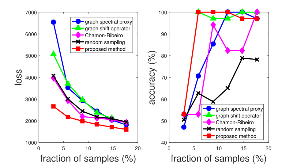
(a) Karate network.

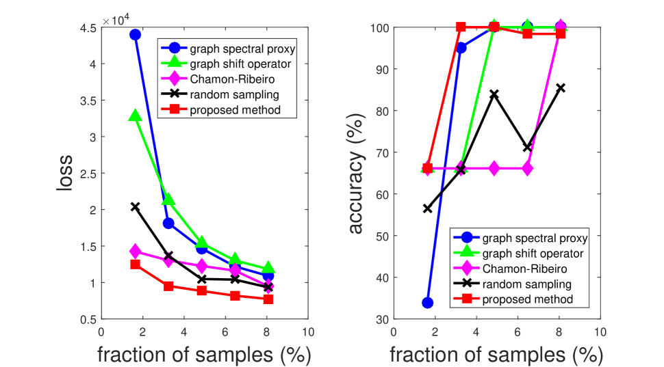
(b) Dolphin network.

Fig. 1: AG-SSL using $\bm{\Omega}_{0}=\mathbf{L}$ and $\sigma^{2}=1/\operatorname{tr}(\bm{\Omega}_{0})$. The proposed method yields perfect community detection by only sampling 2 nodes in each dataset.

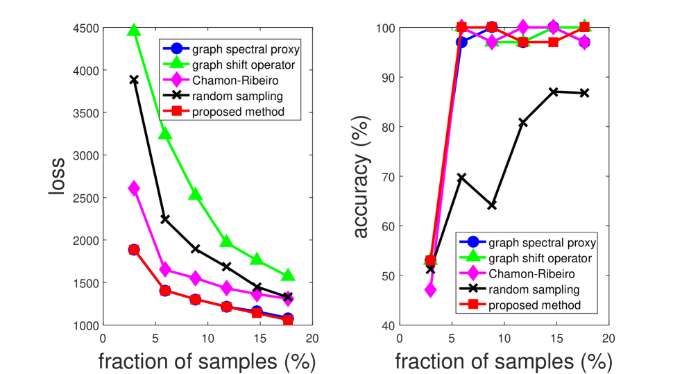
(a) Karate network.

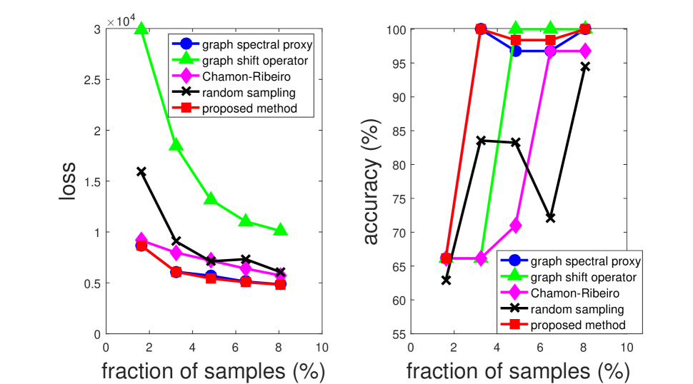
(b) Dolphin network.

Fig. 2: AG-SSL using $\bm{\Omega}_{0}=\mathbf{L}_{N}$ and $\sigma^{2}=1/\operatorname{tr}(\bm{\Omega}_{0})$. The proposed method attains similar performance as in Figure 1. The use of $\mathbf{L}_{N}$ improves the accuracy of GSP and CRM.

4.3 Performance Evaluation

Since AG-SSL on the two community detection datasets discussed in Section 4.1 can be viewed as a semi-supervised binary classification problem, for each method we take the sign of the prediction as the final predicted label. For all methods other than Algorithm 1, we assume that community labels are acquired without noise. For Algorithm 1, to fully comply with the signal model in Section 2, we added an artificial zero-mean Gaussian noise with variance $\sigma^{2}=1/\operatorname{tr}(\bm{\Omega}_{0})$ to the observed labels. The parameter $\sigma^{2}$ can also be viewed as the regularization parameter for the Stieltjes matrix $\bm{\Omega}_{0}$ in (6). Figures 1 and 2 show the loss function value from (5) and the prediction accuracy of different AG-SSL methods using $\bm{\Omega}_{0}=\mathbf{L}$ and $\bm{\Omega}_{0}=\mathbf{L}_{N}$, respectively, where in each curve the markers correspond to the number $s$ of selected samples. It is observed that the proposed method (Algorithm 1) attains the least loss, and Rand may have lower loss than some methods. This is not surprising because the proposed method is designed to minimize the loss via greedy node sampling, while other methods have different objective functions. Nonetheless, for each method except Rand, lower loss is aligned with higher accuracy. The slight fluctuation in the accuracy curve is an artifact of the sign operation for label prediction.

It is worth mentioning that the proposed method can achieve perfect community detection (100% accuracy) by only sampling 2 nodes in each dataset, either using $\mathbf{L}$ or $\mathbf{L}_{N}$ as the regularizer. On the other hand, the other methods may require more samples to achieve the same performance. We also observe that using $\mathbf{L}_{N}$ instead of $\mathbf{L}$ can improve the accuracy of GSP and CRM, which can be explained by the fact that selecting a different $\bm{\Omega}_{0}$ is equivalent to changing the Graph Fourier basis for sampling. To further study different AG-SSL methods, Table 1 displays the fraction of overlapping samples between different sampling strategies when $\bm{\Omega}_{0}=\mathbf{L}$. An interesting finding is that the proposed method has a good amount of overlap with GSP, whereas the samples of GSO and CRM can be very different. Similar relations hold when $\bm{\Omega}_{0}=\mathbf{L}_{N}$. We believe this distinction can be explained by the use of spectral proxy for approximating the actual bandwidth of a graph signal in GSP [20].

5 Conclusion

This paper proved the supermodularity of graph-based SSL under the family of Stieltjes matrix regularization functions, which includes the unnormalized and normalized graph Laplacian matrices that are widely used in graph signal processing. Our analysis yields an efficient greedy AG-SSL algorithm with guaranteed performance relative to the optimum. Evaluated on two community detection datasets, the proposed algorithm outperforms three recent graph signal sampling methods given limited sample budgets. Our future work includes extension to vector-valued labels and joint optimization of the sampling set and the Stieltjes matrix for AG-SSL.

References

• [1] Wei Liu, Jun Wang, and Shih-Fu Chang, โ€œRobust and scalable graph-based semisupervised learning,โ€ Proceedings of the IEEE, vol. 100, no. 9, pp. 2624โ€“2638, 2012.
• [2] Aย Sandryhaila and J.M.F. Moura, โ€œDiscrete signal processing on graphs,โ€ IEEE Trans. Signal Process., vol. 61, no. 7, pp. 1644โ€“1656, Apr. 2013.
• [3] Aliaksei Sandryhaila and Joseย MF Moura, โ€œBig data analysis with signal processing on graphs: Representation and processing of massive data sets with irregular structure,โ€ IEEE Signal Process. Mag., vol. 31, no. 5, pp. 80โ€“90, 2014.
• [4] D.I. Shuman, S.K. Narang, P.ย Frossard, A.ย Ortega, and P.ย Vandergheynst, โ€œThe emerging field of signal processing on graphs: Extending high-dimensional data analysis to networks and other irregular domains,โ€ IEEE Signal Process. Mag., vol. 30, no. 3, pp. 83โ€“98, 2013.
• [5] Akshay Gadde, Aamir Anis, and Antonio Ortega, โ€œActive semi-supervised learning using sampling theory for graph signals,โ€ in ACM International Conference on Knowledge Discovery and Data Mining (KDD), 2014, pp. 492โ€“501.
• [6] Aamir Anis, Alyย El Gamal, Salman Avestimehr, and Antonio Ortega, โ€œA sampling theory perspective of graph-based semi-supervised learning,โ€ arXiv preprint arXiv:1705.09518, 2017.
• [7] Anas Anis, Akshay Gadde, and Antonio Ortega, โ€œTowards a sampling theorem for signals on arbitrary graphs,โ€ in IEEE International Conference on Acoustics, Speech and Signal Processing (ICASSP), 2014, pp. 3864โ€“3868.
• [8] Siheng Chen, Rohan Varma, Aliaksei Sandryhaila, and Jelena Kovaฤeviฤ‡, โ€œDiscrete signal processing on graphs: Sampling theory,โ€ IEEE Trans. Signal Process., vol. 63, no. 24, pp. 6510โ€“6523, 2015.
• [9] Mikhail Belkin, Irina Matveeva, and Partha Niyogi, โ€œRegularization and semi-supervised learning on large graphs,โ€ in International Conference on Computational Learning Theory. Springer, 2004, pp. 624โ€“638.
• [10] Mikhail Belkin, Partha Niyogi, and Vikas Sindhwani, โ€œManifold regularization: A geometric framework for learning from labeled and unlabeled examples,โ€ Journal of machine learning research, vol. 7, no. Nov, pp. 2399โ€“2434, 2006.
• [11] Luizย FO Chamon and Alejandro Ribeiro, โ€œNear-optimality of greedy set selection in the sampling of graph signals,โ€ in IEEE Global Conference on Signal and Information Processing (GlobalSIP), 2016, pp. 1265โ€“1269.
• [12] Luizย FO Chamon and Alejandro Ribeiro, โ€œGreedy sampling of graph signals,โ€ arXiv preprint arXiv:1704.01223, 2017.
• [13] Abraham Berman and Robertย J Plemmons, Nonnegative matrices in the mathematical sciences, SIAM, 1994.
• [14] S.ย Fujishige, Submodular Functions and Optimization, Annals of Discrete Math., North Holland, 1990.
• [15] Santo Fortunato, โ€œCommunity detection in graphs,โ€ Physics Reports, vol. 486, no. 3-5, pp. 75โ€“174, 2010.
• [16] Pin-Yu Chen and Alfredย O. Hero, โ€œLocal Fiedler vector centrality for detection of deep and overlapping communities in networks,โ€ in IEEE International Conference on Acoustics, Speech and Signal Processing (ICASSP), 2014, pp. 1120โ€“1124.
• [17] P.-Y. Chen and A.O. Hero, โ€œDeep community detection,โ€ IEEE Trans. Signal Process., vol. 63, no. 21, pp. 5706โ€“5719, Nov. 2015.
• [18] Wayneย W. Zachary, โ€œAn information flow model for conflict and fission in small groups,โ€ Journal of Anthropological Research, vol. 33, no. 4, pp. 452โ€“473, 1977.
• [19] David Lusseau, Karsten Schneider, OliverJ. Boisseau, Patti Haase, Elisabeth Slooten, and SteveM. Dawson, โ€œThe bottlenose dolphin community of doubtful sound features a large proportion of long-lasting associations,โ€ Behavioral Ecology and Sociobiology, vol. 54, no. 4, pp. 396โ€“405, 2003.
• [20] Aamir Anis, Akshay Gadde, and Antonio Ortega, โ€œEfficient sampling set selection for bandlimited graph signals using graph spectral proxies,โ€ IEEE Trans. Signal Process., vol. 64, no. 14, pp. 3775โ€“3789, 2016.
• [21] Siheng Chen, A.ย Sandryhaila, J.M.F. Moura, and J.ย Kovacevic, โ€œSignal recovery on graphs: Variation minimization,โ€ IEEE Trans. Signal Process., vol. 63, no. 17, pp. 4609โ€“4624, Sept. 2015.