Efficient Graph-based Word Sense Induction
by Distributional Inclusion Vector Embeddings

Abstract

Word sense induction (WSI), which addresses polysemy by unsupervised discovery of multiple word senses, resolves ambiguities for downstream NLP tasks and also makes word representations more interpretable. This paper proposes an accurate and efficient graph-based method for WSI that builds a global non-negative vector embedding basis (which are interpretable like topics) and clusters the basis indexes in the ego network of each polysemous word. By adopting distributional inclusion vector embeddings as our basis formation model, we avoid the expensive step of nearest neighbor search that plagues other graph-based methods without sacrificing the quality of sense clusters. Experiments on three datasets show that our proposed method produces similar or better sense clusters and embeddings compared with previous state-of-the-art methods while being significantly more efficient.

1 Introduction

Word sense induction (WSI) is a challenging task of natural language processing whose goal is to categorize and identify multiple senses of polysemous words from raw text without the help of predefined sense inventory like WordNet (Miller, 1995). The problem is sometimes also called unsupervised word sense disambiguation (Agirre et al., 2006; Pelevina et al., 2016).

An effective WSI has wide applications. For example, we can compare different induced senses in different documents to detect novel senses over time (Lau et al., 2012; Mitra et al., 2014) or analyze sense difference in multiple corpora (Mathew et al., 2017). WSI could also be used to group and diversify the documents retrieved from search engine (Navigli and Crisafulli, 2010; Di Marco and Navigli, 2013). After identifying senses, we can train an embedding for each sense of a word. Li and Jurafsky (2015) demonstrate that this multi-prototype word embedding is useful in several downstream applications including part-of-speech (POS) tagging, relation extraction, and sentence relatedness tasks. Sumanth and Inkpen (2015) also show that word sense disambiguation could be successfully applied to sentiment analysis.

Since word sense induction (WSI) methods are unsupervised, the senses are typically derived from the results of different clustering techniques. Like most of the clustering problems, it is usually challenging to predetermine the number of clusters/senses each word should have. In fact, for many words, the “correct” number of senses is not unique. Setting the number of clusters differently can capture different resolutions of senses. For instance, race in the car context could share the same sense with the race in the game context because they all mean contest, but the race in the car context actually refers to the specific contest of speed. Therefore, they can also be separated into two different senses, depending on the level of granularity we would like to model.

For graph-based clustering methods, it is easy and natural to model the multiple resolutions of senses in a consistent way by hierarchical clustering and defer the difficult problem of choosing the number of clusters to the end. This makes it easier to incorporate other information, such as users’ resolution preference on each hierarchical sense tree. The flexibility is one of the reasons why graph-based methods are widely studied and applied to many downstream applications (Mitra et al., 2014; Mathew et al., 2017; Navigli and Crisafulli, 2010; Di Marco and Navigli, 2013).

Nevertheless, graph-based WSI methods usually require a substantial amount of computational resources. For example, Pelevina et al. (2016) build the graph by finding the nearest neighbors of the target word in the word embedding space (i.e., ego network). Thus, constructing ego networks for all the words takes at least $O(|V|^{2})$ time, where $|V|$ is the size of the vocabulary, unless some approximation is made (e.g., approximate nearest neighbor search such as k-d tree). Next, if our goals include finding less common senses, the method needs to construct a large graph by including more nearest neighbors. For each target word, computing the pairwise distances between nodes in the large graph is also computationally intensive.

To overcome the limitations and make graph-based WSI more practical, we propose a novel WSI algorithm that first groups words into a set of basis indexes (i.e., a set of topics) efficiently and then, constructs the graph where each node corresponds to a basis index (i.e., a topic) instead of a word. The motivation behind the approach is that different senses of a word usually appear in different topics. For example, food and technology will be at least two distinct topics in most of the topic models, so we can find senses by clustering corresponding basis indexes safely when the target word is apple. If one word could have distinct senses in one topic, humans will constantly face difficult word sense disambiguation tasks while reading a document.

Although the main idea is simple, improving the efficiency significantly without sacrificing the quality is difficult. One of the challenges is that similarity between two basis indexes changes given different target words. For example, a country topic should be clustered together with a city topic if the target word is place. However, if the query word is bank, it makes more sense to group the country topic with the money topic into one sense so that the bank mention in Bank of America will belong to the sense. This means we want to focus on the geographical meaning of country when the target word is more about geography, while focus on the economic meaning of country when the target word is more about economics.

In order to tackle the issue, we adopt a recently proposed approach called distributional inclusion vector embedding (DIVE) (Chang et al., 2018). DIVE compresses the sparse bag-of-words while preserving the co-occurrence frequency order, so DIVE is able to model not only the possibility of observing one target word in a topic as typical topic models but also the possibility of observing one topic of a sentence containing a target word mention. This allows us to efficiently identify the topics relevant to each target word, and only focus on an aspect of each of these topics composed of the words relevant to both the topic and the target word.

Experiments show that our method performs similarly compared with Pelevina et al. (2016), a state-of-the-art graph-based WSI method, without the need of expensive nearest neighbor search. Our method is even better for the words without a dominating sense.

2 Related Work

WSI methods can be roughly divided into two categories (Pelevina et al., 2016): clustering words similar to the target/query word or clustering mentions of the target word. We address their general limitations below.

2.1 Clustering Related Words

Graph-based clustering for WSI has a long history and many different variations (Lin et al., 1998; Pantel and Lin, 2002; Dorow and Widdows, 2003; Véronis, 2004; Agirre et al., 2006; Biemann, 2006; Navigli and Crisafulli, 2010; Hope and Keller, 2013; Di Marco and Navigli, 2013; Mitra et al., 2014; Pelevina et al., 2016). In general, the method is to first retrieve words similar or related to each target word as nodes, measure the similarity/relatedness between the words to form an ego graph/network, and either group the nodes by graph clustering or find hubs or representative nodes in the graph using HyperLex (Véronis, 2004) or PageRank (Agirre et al., 2006).

As we mentioned in the introduction section, building word similarity graph and performing graph clustering is usually computationally expensive unless relying on information other than co-occurrence statistics such as word snippets from a search engine (Navigli and Crisafulli, 2010; Di Marco and Navigli, 2013) or existing high-quality dependency parse (Mitra et al., 2014; Pelevina et al., 2016). Depending on the downstream applications and word similarity estimation algorithms available at the time of each work, the methods strive for the balance between efficiency and quality in different ways.

Most of the WSI methods that cluster words use graph-based algorithms. One notable exception is Lau et al. (2012). For each target word, they build a topic model, latent Dirichlet allocation or its extension, on the contexts of all mentions of target words. Although computing pairwise similarity is not required here, the approach is still computationally expensive because there might be tens of thousands of mentions of a target word in the corpus and the approach needs to train $V$ different topic models instead of globally modeling topics once like our method.

In addition to the scalability concerns, we do not know how many mentions of a target word are semantically closest to each of its most related words (i.e., node in its ego-network). The loss of connection makes balance the cluster size during the clustering difficult. Furthermore, it might be common that when users would like to adopt fine-grained senses in the hierarchical clustering tree but realize that there is no mention in the corpus that would be categorized into some sense clusters.

2.2 Clustering Mentions

In addition to clustering words similar/related to the target word, we can also cluster every mention based on its context words, which co-occur in a small window. Although this way saves the time of finding similar words, the samples need to be clustered drastically increase because each target word could have tens of thousands of mentions in the corpus of interest. This makes bottom-up hierarchical clustering or global optimization such as spectral clustering (Stella and Shi, 2003) become infeasible. Without hierarchical sense clustering, it is hard to inject other sources of information such as user intervention or prior knowledge to determine the number of clusters.

To efficiently cluster many samples, Schütze (1992) sub-samples the context of mentions; Mu et al. (2017) run principle component analysis (PCA) to compress the contexts of each target word before clustering; other approaches adopt iteratively local search algorithms after random initialization such as expectation maximization (EM) (Reisinger and Mooney, 2010; Neelakantan et al., 2014; Tian et al., 2014; Piña and Johansson, 2015; Li and Jurafsky, 2015; Bartunov et al., 2016) or gradient descent (Athiwaratkun and Wilson, 2017). Although the random initialization and local search methods could be very efficient, the methods might suffer from bad local minimums. Moreover, the users need to specify the number of senses or a global hyper-parameter which controls the level of granularity at the beginning and hope that it will output the sense models with desired resolution after training finishes. The lack of a way to browsing different sense resolution limits the application of the type of WSI methods.

3 Method

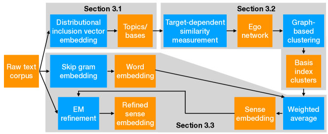
Figure 1: The flowchart of the proposed method. The blue boxes are processing steps, the orange boxes are input and output data of each step, and the gray areas indicate the sections describing the included steps.

The flowchart of our method is illustrated in Figure 1. We will first briefly introduce distributional inclusion vector embedding (DIVE) (Chang et al., 2018) in Section 3.1, illustrate how we use DIVE as a topic model to construct a graph in Section 3.2, and after clustering the topics, we explain the way to converting each topic cluster to a sense embedding in Section 3.3.

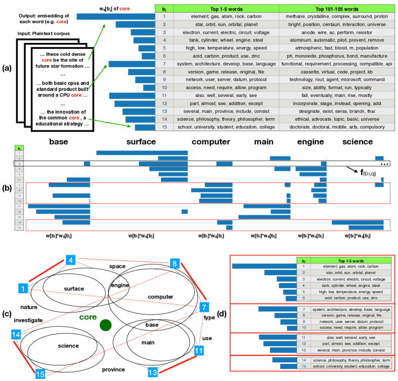
Figure 2: A visualization of finding the senses of the word core.
(a) The DIVE $\mathbf{w}[b_{j}]$ of the word core (only top 15 basis indexes are shown). The words in each row of the table are sorted by its embedding value in the basis index.
(b) Weighted DIVE of six words on these 15 basis indexes relevant to core as the features for measuring the similarity between basis indexes. The two red boxes indicate two final clusters we discovered at the end within which the feature words tend to have similar embedding values.
(c) The ego network constructed for the word core. Each blue box and the corresponding circle represent a basis index or topic (only 8 out of 15 basis indexes are plotted and their index numbers $b_{j}$ are shown in the blue boxes), which is a node in the network. Two basis indexes are more similar if more relevant words (i.e., close to core) occur frequently in both corresponding topics. For example, the topic 7 and 8 are more similar because of the frequent appearance of the relevant words such as computer in both topics. The larger similarity is represented by a thicker red line. The ego network is a complete graph but only a subset of edges are plotted in the figure.
(d) The final clustering results when the number of clusters is set to be 4.

3.1 Distributional Inclusion Vector Embedding (DIVE)

Distributional inclusion vector embedding (DIVE) is a variation of skip-gram model (Mikolov et al., 2013). The two major differences compared with skip-gram are that (1) all word embeddings and context embeddings are constrained to be non-negative, and (2) the weights of negative sampling for each word is inversely proportional to its frequency. Specifically, the objective function of DIVE is defined by

$$l_{DIVE}=\sum_{w}\sum_{c}\#(w,c)\log\sigma(\mathbf{w}^{T}\mathbf{c})~{}+$$ (1)

$$k_{I}\sum_{w}\frac{Z}{\#(w)}\sum_{c}\#(w,c)\underset{c_{N}\sim P_{D}}{\mathbb{E}}[\log\sigma(-\mathbf{w}^{T}\mathbf{c_{N}})],$$

where the word embedding $\mathbf{w}\geq 0$, the context embedding $\mathbf{c}\geq 0,\mathbf{c_{N}}\geq 0$, $\#(w,c)$ are number of times context word $c$ co-occur with $w$, $\#(w)=\sum\limits_{c}\#(w,c)$, $\sigma$ is the logistic sigmoid function, $k_{I}$ is a constant hyper-parameter, $Z$ is the average $\#(w)$ of all words (i.e., $Z=\frac{\sum_{w}\#(w)}{|V|}$ and $|V|$ is the size of vocabulary), and $P_{D}$ is the distribution of negative samples. The two modifications do not change the time and space complexity of training skip-gram, which is one of the most scalable word embedding methods (Levy et al., 2015).

DIVE is originally designed to perform unsupervised hypernymy detection task, and its goal is to preserve the inclusion relation between two context features in the sparse bag of words (SBOW) representation. When the co-occurred context histogram of the word $y$ includes that of the word $x$, it means that for all context words $c$ in the vocabulary $V$, $c$ will co-occur more times with $y$ than with $x$. In this paper, the context words of a target word means the words co-occur with a target word mention within a small window in the corpus. The default context window size for DIVE is 10. Chang et al. (2018) show that the DIVE is able to compress the sparse bag of words while approximately preserving the inclusion in the low-dimensional space. Formally,

$$\forall c\in V,\;\#(x,c)\leq\#(y,c)$$ (2)

$$\tilde{\iff} \forall i\in\{1,...,L\},\;\mathbf{x}[i]\leq\mathbf{y}[i],$$

where $\tilde{\iff}$ means approximately equivalent, $\#(x,c)$ and $\#(y,c)$ are number of times context word $c$ co-occurs with $x$ and $y$, respectively. $\mathbf{x}$ and $\mathbf{y}$ are the embeddings of the words $x$ and $y$, respectively, $\mathbf{x}[i]$ is the embedding value of in $i$th dimension (i.e., $i$th basis index). and $L$ is number of DIVE basis indexes. See Chang et al. (2018) for more the derivation of the equation.

In order to satisfy equation (2), each basis index of DIVE corresponds to a topic and the embedding value at that index represents how often the word appears in the topic. This is because if the embedding of one word $y$ has higher value in every dimension (i.e., higher frequency in every topic) than the value of another word $x$, the context words $c$ in the topics usually co-occur more frequently with $y$ than with $x$. Inversely, if $x$ appears more often in one topic than $y$ (i.e., the embedding value of $x$ in the corresponding dimension is higher than that of $y$), some context words $c$ in the topic could co-occur more often with $x$ than with $y$.

In Figure 2 (a), we present three mentions of the word core and its top 15 basis indexes in DIVE. The word that has a higher value in a basis index is more frequent in the corresponding topic. For example, the top 1-5 words in the second column of the table look more frequent (and usually more general) than the top 101-105 words.

3.2 Graph-Based Clustering

For each target word, we build an ego network whose nodes are the basis indexes relevant to the word. The basis index $b$ is relevant if DIVE of the target word $q$ has a value $\mathbf{w}_{q}[b]$ higher than a threshold $T$. The threshold is set to be $1\%$ of average non-zero $\mathbf{w}_{q}[b]$ over basis indexes in our experiment.

Every pair of nodes are linked by an edge weighted by the similarity between the two basis indexes. Each basis index $b_{i}$ is represented by a feature vector. A naive way to prepare the feature vector of $i$th basis index $\mathbf{f}_{(b_{i})}$ is to use the embedding values in that index $\mathbf{w}[b_{i}]$ of all the words in our vocabulary $V$. That is,

$$\mathbf{f}_{(b_{i})}=\underset{\mathbf{w}\in V}{\oplus}\mathbf{w}[b_{i}],$$ (3)

the operator $\oplus$ means concatenation. However, as discussed in Section 1, measuring similarity using the global features might group topics together based on the co-occurrence of words which are unrelated to the query words. Instead, we want to make the similarity dependent on the query word.

To create target-dependent similarity measurement, we only consider the embedding of words which are related to the query word as the features of basis indexes. Specifically, given a query word $q$, we only take the top $n$ words of every basis index $j$ in the set $B_{j}(n)$ instead of considering all the words in the vocabulary. Then, we weigh the feature based on how likely it is to observe the target word in topic $j$ ($\mathbf{w}_{q}[b_{j}]$) and concatenate all features together. That is, the feature vector of the $i$th dimension $\mathbf{f}_{(b_{i},q)}$ is defined as:

$$\mathbf{f}_{(b_{i},q)}=\overset{L}{\underset{j=1}{\oplus}}\underset{\mathbf{w}\in B_{j}(n)}{\oplus}\mathbf{w}[b_{i}]\cdot\mathbf{w}_{q}[b_{j}],$$ (4)

where $n$ is fixed as 100 in the experiment.

In addition to decreasing the weight of irrelevant words, we also lower the influence of irrelevant bases by defining the similarity between two basis indexes as

$$SIM(b_{i},b_{j},q)= \cos(\mathbf{f}_{(b_{i},q)},\mathbf{f}_{(b_{j},q)})\cdot$$ (5)

$$\log(\frac{\min(\mathbf{w}_{q}[b_{i}],\mathbf{w}_{q}[b_{j}])}{T}),$$

where $\cos(\mathbf{f}_{(b_{i},q)},\mathbf{f}_{(b_{j},q)})$ is the cosine similarity between the features of two basis indexes, and the term $\log(\frac{\min(\mathbf{w}_{q}[b_{i}],\mathbf{w}_{q}[b_{j}])}{T})$ is to prevent irrelevant basis indexes in the ego network misleading the clustering algorithm. Notice that $SIM(b_{i},b_{j},q)\geq 0$ because all features $\mathbf{f}_{(b,q)}\geq 0$ and every node is a relevant basis index $b$ with $\mathbf{w}_{q}[b]>T$.

After the ego network is constructed, we could apply any hierarchical graph clustering. In this paper, we just choose spectral clustering with fixed number of clusters for simplicity. In our experiment, DIVE with 100 dimensions produces only 6.4 relevant basis indexes on average which needs to be clustered for each target word. This number goes to only 19 for DIVE with 300 dimensions. Thus, we are allowed to use spectral clustering to perform global optimization without inducing large computational overhead in this step.

In Figure 2, we use the target word core as an example to illustrate our clustering algorithm. After DIVE is trained in (a), we visualize six dimensions of features for each basis index $\mathbf{f}_{(b_{i},q)}$ in (b). Using the features, we can build the ego network as shown in (c). The figure highlights the novelty of our approach. Instead of directly clustering words as other graph-based methods, we group the words first and cluster the groups to form senses. Since the basis is global, we do not have to retrain it given a different target word. DIVE provides us an easy and efficient way to ignore the irrelevant words being far away from core in (c), such as province or space, and cluster based on the words close to the target word such as main or computer. The target-dependent similarity measurement preserves the main spirit of existing graph-based approaches.

3.3 From Basis Index Clusters to Sense Embeddings

As shown in Figure 2 (d), every sense is represented by a group of basis indexes each of which has a weight based on its relevancy to the target word (e.g., the relevancy of $b_{i}$th basis index is $\mathbf{w}_{q}[b_{i}]$). In order to apply existing WSI evaluation and potentially other downstream applications, we convert the basis index clusters to sense embedding.

First, we train a word embedding. Any existing embeddings could be used and we choose skip-gram due to its efficiency. Based on the trained word2vec, we first create a topic embedding for each basis index by averaging skip-gram embedding of the top 1000 words $B_{i}(1000)$ weighted by the DIVE $\mathbf{w}[b_{i}]$ of the words at $b_{i}$th basis index as given as:

$$\mathbf{t}_{b_{i}}=\frac{\sum_{\mathbf{w}\in B_{i}(1000)}\exp(\mathbf{w^{\prime}}[b_{i}])\cdot\mathbf{e}_{w}}{\sum_{\mathbf{w}\in B_{i}(1000)}\exp(\mathbf{w^{\prime}}[b_{i}])},$$ (6)

where $\mathbf{e}_{w}$ is the skip-gram embedding for the word whose DIVE are $\mathbf{w}$, and $\mathbf{w^{\prime}}$ is normalized DIVE such that its average $\frac{\sum_{\mathbf{w}\in B_{i}(1000)}\mathbf{w^{\prime}}[b_{i}]}{1000}=1$. We take exponential on $\mathbf{w^{\prime}}[b_{i}]$ to focus on the words that are more important to the $b_{i}$ basis index because DIVE roughly models the $\log$ of word frequency in each topic (Chang et al., 2018).

To generate $k$th sense embedding $\mathbf{s}^{q}_{k}$ for a target word $q$, we take the average of all the topic embeddings in the $k$th sense cluster (found in Section 3.2) weighted by the relevancy between every topic and the target word. Specifically,

$$\mathbf{s}^{q}_{k}=\frac{\sum_{b_{i}\in S^{q}_{k}}\exp(\mathbf{w^{\prime}}_{q}[b_{i}])\cdot\mathbf{t}_{b_{i}}}{\sum_{b_{i}\in S^{q}_{k}}\exp(\mathbf{w^{\prime}}_{q}[b_{i}])},$$ (7)

where $S^{q}_{k}$ is the set of basis indexes that belongs to the $k$th cluster, $\mathbf{w^{\prime}}_{q}$ is normalized DIVE of the target word such that its average $\frac{\sum_{b_{i}\in N}\mathbf{w^{\prime}}_{q}[b_{i}]}{|N|}=1$, and $N$ is the set of nodes in the ego network.

When converting clusters into embeddings, the previous graph-based WSI methods, such as  Pelevina et al. (2016), average the embedding of related words. The average is effective in terms of discriminating the contexts of target word mentions, but it might not be a good embedding for the sense of target word itself. For instance, one sense embedding of core could be close to the embedding of computer, but the computer embedding does not represent the sense of core in computer context as well as the embedding of cpu. Our method suffers the similar problem.

To solve the issue, we use the sense embeddings from clusters as the initialization of an expectation maximization (EM) refinement. At E-step, we predict the sense of every target token by checking which sense embedding the average word embedding of the current sentence is closest to, and assign the sense to the target token (e.g., bank $\rightarrow$ bank_1). At M-step, we retrain the skip-gram using the updated corpus. Our refinement process could be seen as a simplified version of multi-sense skip-gram (MSSG) (Neelakantan et al., 2014), which can be easily implemented using existing word embedding library.

4 Experiments

We first conduct a qualitative experiment to verify that our clustering algorithm performs well on some typical polysemy, and show the results in Table 1. As we can see, our method can not only separate two senses in very different contexts but also can distinguish more subtle sense difference such as identifying the car context and competition context as two different senses of the target word race.

Intuitively speaking, our method could be especially useful when it comes to increase the recall of less common senses (like discovering the educational meaning of core), but it is hard to verify the claim using existing WSI benchmarks because the common senses, especially the most frequent sense, often dominate in the benchmarks unless using the datasets where the bias is removed. In the following sections, we will first introduce the setup and then the experiments on 3 datasets.

Query	CID	Top 5 words in the top dimensions
rock	1	element, gas, atom, rock, carbon	sea, lake, river, area, water
		find, specie, species, animal, bird	point, side, line, front, circle
	2	band, song, album, music, rock	write, john, guitar, band, author
		early, work, century, late, begin	include, several, show, television, film
bank	1	county, area, city, town, west	several, main, province, include, consist
		building, build, house, palace, site	sea, lake, river, area, water
	2	money, tax, price, pay, income	company, corporation, system, agency, service
		united, states, country, world, europe	state, palestinian, israel, right, palestine
apple	1	food, fruit, vegetable, meat, potato	goddess, zeus, god, hero, sauron
		war, german, ii, germany, world	write, john, guitar, band, author
	2	version, game, release, original, file	car, company, sell, manufacturer, model
		system, architecture, develop, base, language	include, several, show, television, film
star	1	film, role, production, play, stage	character, series, game, novel, fantasy
		wear, blue, color, instrument, red	write, john, guitar, band, author
	2	element, gas, atom, rock, carbon	star, orbit, sun, orbital, planet
		give, term, vector, mass, momentum	light, image, lens, telescope, camera
tank	1	tank, cylinder, wheel, engine, steel	industry, export, industrial, economy, company
		acid, carbon, product, use, zinc	network, user, server, datum, protocol
	2	army, force, infantry, military, battle	aircraft, navy, missile, ship, flight
		however, attempt, result, despite, fail	war, german, ii, germany, world
race	1	win, world, cup, play, championship	two, one, three, four, another
	2	railway, line, train, road, rail	car, company, sell, manufacturer, model
	3	population, language, ethnic, native, people	female, age, woman, male, household
run	1	system, architecture, develop, base, language	access, need, require, allow, program
	2	railway, line, train, road, rail	also, well, several, early, see
	3	game, team, season, win, league	game, player, run, deal, baseball
tablet	1	bc, source, greek, ancient, date	book, publish, write, work, edition
	2	use, system, design, term, method	version, game, release, original, file
	3	system, blood, vessel, artery, intestine	patient, symptom, treatment, disorder, may

Table 1: Examples of sense clusters on polysemous words. When the number of clusters is set to be 2, we present the top 4 basis indexes $b_{j}$ in each sense cluster, which have the highest values on the target word embedding $\mathbf{w}_{q}[b_{j}]$. Otherwise, the top 2 basis indexes are presented. CID refers to sense cluster ID. The top 5 words with the highest values of each basis index $\mathbf{w}[b_{j}]$ are presented.

4.1 Experimental Setup

We train DIVE on first 51.2 million tokens of WaCkypedia (Baroni et al., 2009), the dataset suggested by Chang et al. (2018), and the default hyper-parameter setting is used except the number of embedding dimensions $L$ (i.e., number of basis indexes). We train two DIVEs, one with 100 dimensions and the other with 300 dimensions to study how the granularity of basis affects the performance. For all other steps or baselines, we train them on the whole WaCkypedia where the stop words are removed.

For our clustering module, we use all the default hyper-parameters of the spectral clustering library in Scikit-learn 0.18.2 (Pedregosa et al., 2011) except the number of clusters is fixed at 2. Setting a number larger than 2 makes it harder to compare with the results generated from other baselines whose default hyper-parameters usually make average number of senses between 1 and 2. During EM, we train the skip-gram embedding on the whole WaCkypedia where we treat every consecutive 20 tokens as a sentence, and the refinement stops after 3 EM iteration. In the tables of this section, our methods using DIVE with 100 and 300 dimensions are denoted as DIVE (100) and DIVE (300), respectively.

In all quantitative experiments, we compare our method with Pelevina et al. (2016), a state-of-the-art graph-based clustering which builds ego graphs based on words similar to the target words, so we call it word graph (WG). To train the model, we first train skip-gram on whole WaCkypedia and use all the default hyper-parameters in their released code to get sense embeddings. We also apply our EM refinement step to their output embedding to make the comparison fair and call this variation WG+EM. We also compare our method with the baseline which randomly assigns two senses to every token and performs EM to refine the embedding (i.e., only adopting our post-processing step). The method is similar to multiple-sense skip-gram (Neelakantan et al., 2014), so we call it MSSG in our tables.

In all datasets, evaluation involves the similarity measurement between a sense of the target word and a context. For each query, we compute cosine similarity between the context embedding and the sense embedding of the target word, where the context embedding $\mathbf{e}_{c}$ is the average embedding of word in the context. Notice that each word in the context could also be polysemous. In these cases, we adopt the sense embedding of the context word that is closest to the sense of the target word (i.e., highest cosine similarity).

4.2 Word Context Relevance (WCR)

Given a target word, the task (Arora et al., 2016; Sun et al., 2017) is to identify the true context corresponding to a sense of the target word out of 10 other randomly selected false contexts, where a context is presented by similar words. For example, two of the true contexts for the target word bank are water,land,river,… and institution,deposits,money…. We use the R1 dataset from Sun et al. (2017), which consists of 137 word types and 535 queries.

For each query pair (target word $w_{q}$, context $c$), we compute the similarity between each sense of target word $\mathbf{s}^{q}_{k}$ and the context $\mathbf{e}_{c}$, and choose the senses of the target word with maximal similarity (i.e., $SIM(w_{q},\mathbf{e}_{c})=\max_{k}\cos(\mathbf{s}^{q}_{k},\mathbf{e}_{c})$). Then, we rank the similarity of 11 query pairs, which consist of 1 true context and 10 false contexts. The performance of different methods is evaluated by checking whether the top 1 (i.e., the pair with the highest similarity) is true. The metric (Sun et al., 2017) is called Precision@1.

The results are shown in Table 2. Since the task is to identify the related contexts, skip-gram is a good baseline (Sun et al., 2017). In this dataset, each sense is equally important, regardless how often the sense appears in the corpus. The significantly better performance from DIVE demonstrates our capability of modeling more fine-grained senses of polysemous words.

Skip-gram	WG	WG+EM
52.7	42.1	59.1
MSSG	DIVE (100)	DIVE (300)
60	63.2	62.6

Table 2: Precision@1 on the WCR R1 (%).

Model	TWSI			balanced TWSI
	P	R	F1	P	R	F1
MSSG rnd	66.1	65.7	65.9	33.9	33.7	33.8
MSSG	66.2	65.8	66.0	34.3	34.2	34.2
WG	68.6	68.1	68.4	38.7	38.5	38.6
WG+EM	68.3	67.8	68.0	38.4	38.2	38.3
DIVE rnd	63.4	63.0	63.2	33.4	33.2	33.3
DIVE (100)	67.6	67.2	67.4	39.7	39.5	39.6
DIVE (300)	67.4	66.9	67.2	39.0	38.8	38.9

Table 3: Results obtained on the TWSI task (%), where P is precision and R is recall. MSSG rnd and DIVE rnd are baselines which randomly assign sense given inventory built by MSSG and DIVE, respectively.

Model	JI	Tau	WNDCG	FNMI	FB-C
All-1	19.2	60.9	28.8	0	62.3
Rnd	21.8	62.8	28.7	2.8	47.4
MSSG	22.2	62.9	29.0	3.2	48.9
WG	21.2	61.2	29.0	1.6	58.1
WG+EM	21.0	61.5	29.0	1.3	57.8
DIVE (100)	21.9	61.9	29.3	3.1	50.6
DIVE (300)	22.1	62.8	29.1	3.5	49.9

Table 4: Results obtained on the SemEval 2013 task (%), where JI is Jaccard Index, FNMI is Fuzzy NMI, and FB-C is Fuzzy B-Cubed. All-1 is to assign all senses to be the same and Rnd is to randomly assign all senses to 2 groups.

4.3 TWSI Evaluation

The Turk bootstrap Word Sense Inventory (TWSI) task (Biemann, 2012) is based on a large dataset, which consists of 1,012 nouns accompanied with 145,140 context sentences. The task is to identify the correct sense of the target nouns, and all WSI algorithms choose the sense whose embedding is most similar to the context embedding.

Dataset is heavily skewed with 79% of contexts being assigned to the most frequent senses. To remove this bias, we follow the procedure described in Pelevina et al. (2016) to create balanced TWSI. Specifically, we only keep the first 5 contexts of each sense of every target word to make every sense count equally. The procedure yields 8710 pairs of senses and contexts.

When evaluating on TWSI, each method needs to represent the sense by a sparse bag-of-word context feature called sense inventory. The evaluation script first maps each sense predicted by each algorithm to a ground truth sense. Then, the problem becomes a classification task, which can be evaluated by precision, recall, and F1.

In Table 3, we can see that DIVE performs slightly worse than WG (Pelevina et al., 2016) in full TWSI, but becomes slightly better in balanced TWSI. We suspect this is because our number of sense is 2 but the WG generates the output where the average number of senses is around 1.5, which might do better when a sense of each word occurs most of the time. Notice that the comparison in balanced TWSI is fair because the experiments in Pelevina et al. (2016) show that WG performs worse when increasing number of clusters. The results also suggest that a sufficient number of basis vectors seldom group two senses together (otherwise, increasing the resolution/dimension of DIVE should be helpful).

4.4 SemEval-2013 task 13 Evaluation

SemEval-2013 task 13 (Jurgens and Klapaftis, 2013) provides a smaller dataset which consists of 50 words which include nouns, verbs, and adjectives. The context prediction is done in the same way as TWSI, and the meaning of each metric could be found in Jurgens and Klapaftis (2013). In Table 4, we can see our method performs roughly the same compared with other baselines.

5 Conclusions

We propose a novel graph-based WSI approach. In order to save the time of performing a nearest neighbor search, we first group words into basis/topics using distributional inclusion vector embedding (DIVE), compute target-dependent similarity between basis indexes, and then perform graph clustering. Our experimental results show that the method achieves the state-of-the-art performances and is able to capture less common senses with higher accuracy.

6 Acknowledgement

This material is based upon work supported in part by the Center for Data Science and the Center for Intelligent Information Retrieval, in part by Lexalytics, in part by the Chan Zuckerberg Initiative under the project Scientific Knowledge Base Construction, and in part by the National Science Foundation under Grant No. IIS-1514053 and No. DMR-1534431, in part using high performance computing equipment obtained under a grant from the Collaborative R&D Fund managed by the Massachusetts Technology Collaborative. Any opinions, findings and conclusions or recommendations expressed in this material are those of the authors and do not necessarily reflect those of the sponsor.

References

- Agirre et al. (2006) Eneko Agirre, David Martínez, Oier Lopez de Lacalle, and Aitor Soroa. 2006. Two graph-based algorithms for state-of-the-art WSD. In EMNLP 2007, Proceedings of the 2006 Conference on Empirical Methods in Natural Language Processing, 22-23 July 2006, Sydney, Australia.
- Arora et al. (2016) Sanjeev Arora, Yuanzhi Li, Yingyu Liang, Tengyu Ma, and Andrej Risteski. 2016. Linear algebraic structure of word senses, with applications to polysemy. arXiv preprint arXiv:1601.03764 .
- Athiwaratkun and Wilson (2017) Ben Athiwaratkun and Andrew Gordon Wilson. 2017. Multimodal word distributions. In ACL.
- Baroni et al. (2009) Marco Baroni, Silvia Bernardini, Adriano Ferraresi, and Eros Zanchetta. 2009. The WaCky wide web: a collection of very large linguistically processed web-crawled corpora. Language resources and evaluation 43(3):209–226.
- Bartunov et al. (2016) Sergey Bartunov, Dmitry Kondrashkin, Anton Osokin, and Dmitry P. Vetrov. 2016. Breaking sticks and ambiguities with adaptive skip-gram. In Proceedings of the 19th International Conference on Artificial Intelligence and Statistics, AISTATS 2016, Cadiz, Spain, May 9-11, 2016.
- Biemann (2006) Chris Biemann. 2006. Chinese whispers: an efficient graph clustering algorithm and its application to natural language processing problems. In Proceedings of the first workshop on graph based methods for natural language processing.
- Biemann (2012) Chris Biemann. 2012. Turk bootstrap word sense inventory 2.0: A large-scale resource for lexical substitution. In Proceedings of the Eighth International Conference on Language Resources and Evaluation, LREC 2012, Istanbul, Turkey, May 23-25, 2012.
- Chang et al. (2018) Haw-Shiuan Chang, ZiYun Wang, Luke Vilnis, and Andrew McCallum. 2018. Distributional inclusion vector embedding for unsupervised hypernymy detection. In Human Language Technology Conference of the North American Chapter of the Association of Computational Linguistics (HLT/NAACL).
- Di Marco and Navigli (2013) Antonio Di Marco and Roberto Navigli. 2013. Clustering and diversifying web search results with graph-based word sense induction. Computational Linguistics 39(3):709–754.
- Dorow and Widdows (2003) Beate Dorow and Dominic Widdows. 2003. Discovering corpus-specific word senses. In EACL 2003, 10th Conference of the European Chapter of the Association for Computational Linguistics, April 12-17, 2003, Agro Hotel, Budapest, Hungary.
- Hope and Keller (2013) David Hope and Bill Keller. 2013. Maxmax: a graph-based soft clustering algorithm applied to word sense induction. In International Conference on Intelligent Text Processing and Computational Linguistics.
- Jurgens and Klapaftis (2013) David Jurgens and Ioannis Klapaftis. 2013. Semeval-2013 task 13: Word sense induction for graded and non-graded senses. In Second Joint Conference on Lexical and Computational Semantics (* SEM), Volume 2: Proceedings of the Seventh International Workshop on Semantic Evaluation (SemEval 2013).
- Lau et al. (2012) Jey Han Lau, Paul Cook, Diana McCarthy, David Newman, and Timothy Baldwin. 2012. Word sense induction for novel sense detection. In EACL 2012, 13th Conference of the European Chapter of the Association for Computational Linguistics, Avignon, France, April 23-27, 2012.
- Levy et al. (2015) Omer Levy, Yoav Goldberg, and Ido Dagan. 2015. Improving distributional similarity with lessons learned from word embeddings. Transactions of the Association for Computational Linguistics 3:211–225.
- Li and Jurafsky (2015) Jiwei Li and Dan Jurafsky. 2015. Do multi-sense embeddings improve natural language understanding? In Proceedings of the 2015 Conference on Empirical Methods in Natural Language Processing, EMNLP 2015, Lisbon, Portugal, September 17-21, 2015.
- Lin et al. (1998) Dekang Lin et al. 1998. An information-theoretic definition of similarity. In ICML.
- Mathew et al. (2017) Binny Mathew, Suman Kalyan Maity, Pratip Sarkar, Animesh Mukherjee, and Pawan Goyal. 2017. Adapting predominant and novel sense discovery algorithms for identifying corpus-specific sense differences. In Proceedings of TextGraphs@ACL 2017: the 11th Workshop on Graph-based Methods for Natural Language Processing, Vancouver, Canada, August 3, 2017.
- Mikolov et al. (2013) Tomas Mikolov, Ilya Sutskever, Kai Chen, Greg S Corrado, and Jeff Dean. 2013. Distributed representations of words and phrases and their compositionality. In NIPS.
- Miller (1995) George A. Miller. 1995. Wordnet: a lexical database for english. Communications of the ACM 38(11):39–41.
- Mitra et al. (2014) Sunny Mitra, Ritwik Mitra, Martin Riedl, Chris Biemann, Animesh Mukherjee, and Pawan Goyal. 2014. That’s sick dude!: Automatic identification of word sense change across different timescales. In Proceedings of the 52nd Annual Meeting of the Association for Computational Linguistics, ACL 2014, June 22-27, 2014, Baltimore, MD, USA, Volume 1: Long Papers.
- Mu et al. (2017) Jiaqi Mu, Suma Bhat, and Pramod Viswanath. 2017. Geometry of polysemy. In ICLR.
- Navigli and Crisafulli (2010) Roberto Navigli and Giuseppe Crisafulli. 2010. Inducing word senses to improve web search result clustering. In Proceedings of the 2010 conference on empirical methods in natural language processing.
- Neelakantan et al. (2014) Arvind Neelakantan, Jeevan Shankar, Alexandre Passos, and Andrew McCallum. 2014. Efficient non-parametric estimation of multiple embeddings per word in vector space. In Proceedings of the 2014 Conference on Empirical Methods in Natural Language Processing, EMNLP 2014, October 25-29, 2014, Doha, Qatar, A meeting of SIGDAT, a Special Interest Group of the ACL.
- Pantel and Lin (2002) Patrick Pantel and Dekang Lin. 2002. Discovering word senses from text. In Proceedings of the eighth ACM SIGKDD international conference on Knowledge discovery and data mining.
- Pedregosa et al. (2011) F. Pedregosa, G. Varoquaux, A. Gramfort, V. Michel, B. Thirion, O. Grisel, M. Blondel, P. Prettenhofer, R. Weiss, V. Dubourg, J. Vanderplas, A. Passos, D. Cournapeau, M. Brucher, M. Perrot, and E. Duchesnay. 2011. Scikit-learn: Machine learning in Python. Journal of Machine Learning Research 12(Oct):2825–2830.
- Pelevina et al. (2016) Maria Pelevina, Nikolay Arefiev, Chris Biemann, and Alexander Panchenko. 2016. Making sense of word embeddings. In Proceedings of the 1st Workshop on Representation Learning for NLP, Rep4NLP@ACL 2016, Berlin, Germany, August 11, 2016.
- Piña and Johansson (2015) Luis Nieto Piña and Richard Johansson. 2015. A simple and efficient method to generate word sense representations. In Recent Advances in Natural Language Processing, RANLP 2015, 7-9 September, 2015, Hissar, Bulgaria.
- Reisinger and Mooney (2010) Joseph Reisinger and Raymond J. Mooney. 2010. Multi-prototype vector-space models of word meaning. In Human Language Technologies: Conference of the North American Chapter of the Association of Computational Linguistics, Proceedings, June 2-4, 2010, Los Angeles, California, USA.
- Schütze (1992) Hinrich Schütze. 1992. Dimensions of meaning. In Proceedings of the 1992 ACM/IEEE conference on Supercomputing.
- Stella and Shi (2003) X Yu Stella and Jianbo Shi. 2003. Multiclass spectral clustering. In ICCV.
- Sumanth and Inkpen (2015) Chiraag Sumanth and Diana Inkpen. 2015. How much does word sense disambiguation help in sentiment analysis of micropost data? In Proceedings of the 6th Workshop on Computational Approaches to Subjectivity, Sentiment and Social Media Analysis.
- Sun et al. (2017) Yifan Sun, Nikhil Rao, and Weicong Ding. 2017. A simple approach to learn polysemous word embeddings. arXiv preprint arXiv:1707.01793 .
- Tian et al. (2014) Fei Tian, Hanjun Dai, Jiang Bian, Bin Gao, Rui Zhang, Enhong Chen, and Tie-Yan Liu. 2014. A probabilistic model for learning multi-prototype word embeddings. In COLING.
- Véronis (2004) Jean Véronis. 2004. Hyperlex: lexical cartography for information retrieval. Computer Speech & Language 18(3):223–252.