Charge density wave and charge pump of interacting fermions in circularly shaken hexagonal optical lattices

Abstract

We analyze strong correlation effects and topological properties of interacting fermions with a Falicov-Kimball type interaction in circularly shaken hexagonal optical lattices, which can be effectively described by the Haldane-Falicov-Kimball model, using the real-space Floquet dynamical mean-field theory (DMFT). The Haldane model, a paradigmatic model of the Chern insulator, is experimentally relevant, because it has been realized using circularly shaken hexagonal optical lattices. We show that in the presence of staggering a charge density wave emerges, which is affected by interactions and resonant tunneling. We demonstrate that interactions smear out the edge states by introducing a finite life time of quasiparticles. Even though a general method for calculating the topological invariant of a nonequilibrium steady state is lacking, we extract the topological invariant using a Laughlin charge pump set-up. We find and attribute to the dissipations into the bath connected to every lattice site, which is intrinsic to real-space Floquet DMFT methods, that the pumped charge is not an integer even for the non-interacting case at very low reservoir temperatures. Furthermore, using the rate equation based on the Floquet-Born-Markov approximation, we calculate the charge pump from the rate equations for the non-interacting case to identify the role of the spectral properties of the bath. Starting from this approach we propose an experimental protocol for measuring quantized charge pumping.

I Introduction

Time periodically driven ultracold atoms in optical lattices are a versatile and powerful platform to simulate models with non-trivial topological properties Eckardt (2017); Goldman et al. (2016). Two paradigmatic models, the Hofstadter model and the Haldane model have been realized with Raman laser assisted tunneling Aidelsburger et al. (2013); Miyake et al. (2013); Aidelsburger et al. (2015) and circularly shaken hexagonal lattices Jotzu et al. (2014); Fläschner et al. (2016, 2017), respectively. Different techniques have been developed in setups with ultracold atoms in optical lattices to detect topological properties. Using a drift measurement, the topology of the lowest band of the Hofstadter model was determined Aidelsburger et al. (2015). By measuring the shift of atom clouds in a one-dimensional superlattice, the Thouless charge pump was realized in bosonic Lu et al. (2016); Lohse et al. (2016) and fermionic Nakajima et al. (2016) systems. A two-dimensional version of the topological charge pump was demonstrated by mapping a four-dimensional quantum Hall system to a two-dimensional square superlattice using dimensional reduction Lohse et al. (2018). Using the tomographic technique that was proposed in Ref. Hauke et al. (2014), the Berry curvature of the Haldane model was mapped out in momentum space Fläschner et al. (2016). Also, dynamical vortices due to quenching into the Floquet Hamiltonian were observed Fläschner et al. (2017), which are a non-equilibrium signature of topology. The trajectories of the dynamical vortices in momentum space were used to determine the linking number Tarnowski et al. (2017), which can be directly related to the Chern number of the Hamiltonian after a quench Wang et al. (2017). So far, one can understand most experimental achievements Jotzu et al. (2014); Fläschner et al. (2016, 2017); Tarnowski et al. (2017) with non-interacting effective Hamiltonians Bukov et al. (2015a).

Introducing two-particle interactions into a time-periodically driven system is a highly non-trivial problem from the point of view of both experiment and theory. In experiments one needs to overcome the problem of heating. It was shown that an interacting time-periodically driven closed system will heat up to a trivial state with infinite temperature D’Alessio and Rigol (2014); Lazarides et al. (2014a), with only a few exceptions like many-body localized systems Ponte et al. (2015); Lazarides et al. (2015), integrable systems Lazarides et al. (2014b) and the prethermalization plateau Bukov et al. (2015b); Weidinger and Knap (2017). Multi-photon interband heating has been observed in a shaken 1D optical lattice Weinberg et al. (2015). Resonant tunneling, which happens when interactions are integer multiples of the driving frequency and magnetic correlations have been measured for strongly correlated fermions in hexagonal optical lattices with periodic driving in one direction Görg et al. (2018). Floquet evaporative cooling was shown to reduce heating for interacting bosons in a one-dimensional optical lattice Reitter et al. (2017). However, there are no artificial gauge fields in these setups. Further efforts are needed to go into the interacting regime and realize an interacting system with artificial gauge fields. Theoretically, in the high-frequency limit, where the time periodically driven system is supposed to be in a prethermalized regime Bukov et al. (2015b), the system can be described by an effective Hamiltonian in high-frequency approximation Goldman and Dalibard (2014); Bukov et al. (2015a); Eckardt and Anisimovas (2015). With interactions turned on, the interacting Haldane model can be studied with the static mean-field approximation Zheng et al. (2015); Plekhanov et al. (2017) and exact diagonalization Anisimovas et al. (2015). The possible drawback of the effective Hamiltonian approach is that it cannot describe the non-equilibrium properties of the system. In the strongly correlated regime, one can obtain the effective low-energy Hamiltonian in the limit of large interaction using a high-frequency expansion, which is equivalent to a Schrieffer-Wolff transformation Bukov et al. (2016). With it one can qualitatively analyze the properties of near-resonant and resonant tunneling. However, to solve the low energy effective Hamiltonian is still a very non-trivial many-body problem. Numerical tools such as quantum Monte-Carlo and density matrix renormalization method need to be adopted to solve it.

Based on the experimental progress Fläschner et al. (2016, 2017); Tarnowski et al. (2017), we investigate non-equilibrium steady states (NESS) of fermions with Falicov-Kimball type interactions in a circularly shaken hexagonal optical lattice in a non-perturbative way using the method of real-space Floquet dynamical mean field theory (DMFT) Freericks et al. (2006); Tsuji et al. (2008); Joura et al. (2008); Freericks and Joura (2008); Aoki et al. (2014), which can deal with driving, interactions and dissipation on equal footing. We study the strong correlation effects and topological properties of the system. We investigate the charge density wave (CDW) induced by the staggered potential as a function of increasing interactions. To study topological properties, we use a Laughlin charge pump setup Laughlin (1981), where a flux is inserted in the direction of the axis of a cylinder geometry. We observe how the edge states are smeared out by interactions. Furthermore, we calculate the charge pump due to insertion of flux quanta for different interactions. The dissipation into the bath makes the pumped charge non-integer. In addition, we study the role of dissipation for the non-interacting case in the presence of a heat bath using rate equations based on the Floquet-Born-Markov approximation. We start from an initial state which is close to equilibrium, and ramp up the flux adiabatically to calculate the pumped charge. By comparison with the equilibrium case we believe our procedure is experimentally practical.

We include a bath in all our calculations. While the bath prevents serious heating of the driven system, it causes dissipation which smears the integer charge pump, at least within our theoretical approaches for dealing with the bath. Whether it is possible to recover the integer charge pump by bath engineering will be a future direction.

The manuscript is organized as follows. In Sec. II, we present the model and methods used in our calculations. We outline the real-space Floquet DMFT method for the interacting and driven system, and the rate equation for the non-interacting case. In Sec. III, we present our results on the charge density wave and charge pump for the interacting system. For the non-interacting case, we show calculations from rate equations. We conclude in Sec. IV.

II Model and methods

II.1 The model

We start with a model for fermions in circularly shaken hexagonal optical lattices which can describe the experimental setups described in Refs. Fläschner et al. (2016, 2017); Tarnowski et al. (2017); Sohal and Eckardt (2016)

$$H_{0}=-J\sum_{\left\langle ll^{\prime}\right\rangle}c_{l^{\prime}}^{\dagger}c_{l}+\sum_{l}\nu_{l}\left(t\right)n_{l}+\alpha\left(\Omega+\Delta\right)\sum_{l}\lambda_{l}n_{l},$$ (1)

where $l$ and $l^{\prime}$ label lattices sites, and $n_{l}=c_{l}^{\dagger}c_{l}$. $\Omega$ is the driving frequency and $\Delta$ is the detuning between the driving frequency and the AB-offset in the static lattice. $\lambda_{\mathrm{A}\left(\mathrm{B}\right)}=0\left(1\right)$ for A and B sites in the unit-cell. $\alpha=\pm 1$ which is the sign of the staggered potential. We consider a near-resonant driving, which reestablishes resonant tunneling between A and B sites. The driving term is given by $\nu_{l}\left(t\right)=-\bm{r}_{l}\cdot\bm{F}\left(t\right)=-\bm{r}_{l}\cdot F\left[\cos\left(\Omega t\right)\hat{\bm{e}}_{x}+\tau\sin\left(\Omega t\right)\hat{\bm{e}}_{y}\right]$, where $\tau=\pm 1$ corresponds to counter-clockwise (clockwise) shaking. In the following, we choose $\alpha=1$ and $\tau=1$. For the Schrödinger equation of the system $i\frac{d\left|\psi\right\rangle}{dt}=H_{0}\left|\psi\right\rangle$, with the unitary transformation $\left|\psi\right\rangle=\mathcal{U}\left|\tilde{\psi}\right\rangle$ and $\mathcal{U}=e^{i\sum_{l}\tilde{\chi}_{l}\left(t\right)n_{l}}$, where

$$\tilde{\chi}_{l}\left(t\right) =-\int_{0}^{t}\tilde{\nu}_{l}\left(t\right)dt+\frac{1}{\mathcal{T}}\int_{0}^{\mathcal{T}}dt^{\prime\prime}\int_{0}^{t^{\prime\prime}}dt^{\prime}\tilde{\nu}_{l}\left(t^{\prime}\right),$$ (2)

$$\tilde{\nu}_{l}\left(t\right) =\nu_{l}\left(t\right)+\alpha\Omega\lambda_{l},$$ (3)

and $\mathcal{T}=\frac{2\pi}{\Omega}$, we have $\tilde{H}_{0}=\mathcal{U}^{\dagger}H_{0}\mathcal{U}-i\mathcal{U}^{\dagger}\frac{d}{dt}\mathcal{U}$. Therefore,

$$\tilde{H}_{0}(t)=-J\sum_{\left\langle ll^{\prime}\right\rangle}e^{i\tilde{\theta}_{l^{\prime}l}\left(t\right)}c_{l^{\prime}}^{\dagger}c_{l}+\alpha\Delta\sum_{l}\lambda_{l}n_{l}$$ (4)

where $\tilde{\theta}_{l^{\prime}l}\left(t\right)=\frac{K}{\Omega}\sin\left(\Omega t-\tau\phi_{l^{\prime}l}\right)+\alpha\epsilon_{l^{\prime}l}\Omega t-\alpha\epsilon_{l^{\prime}l}\pi$. $\phi_{l^{\prime}l}$ is defined by $\bm{r}_{l^{\prime}}-\bm{r}_{l}=\cos\left(\phi_{l^{\prime}l}\right)\hat{\bm{e}}_{x}+\sin\left(\phi_{l^{\prime}l}\right)\hat{\bm{e}}_{y}$ for nearest neighbors.

We consider a Falicov-Kimball interaction, where the mobile atoms interact with localized atoms:

$$H_{\mathrm{int}}=U\sum_{l}c_{l}^{\dagger}c_{l}f_{l}^{\dagger}f_{l}.$$ (5)

$U$ is the interaction strength. $f_{l}$ ($f_{l}^{\dagger}$) is the annihilation (creation) operator for localized atoms. $f$-atoms work as an annealed disorder for the mobile atoms. The interaction term $H_{\mathrm{int}}$ is not affected by the driving term in Eq. (1), because it commutes with the driving term.

II.2 Real-space Floquet DMFT

We outline the real-space Floquet DMFT method that we adopt to deal with the Falicov-Kimball interaction Freericks et al. (2006); Tsuji et al. (2008); Tsuji (2010); Qin and Hofstetter (2017). It is a method to study the NESS in an inhomogeneous system. To reach the NESS, every lattice site is coupled to a bath. We use a free-fermion bath in our implementation Tsuji et al. (2009); Aoki et al. (2014). The full Green’s function of the lattice system satisfies Dyson’s equation,

$$\left(\hat{G}^{-1}\right)_{ll^{\prime},mn}\left(\omega\right)= \left(\hat{G}_{0}^{-1}\right)_{ll^{\prime},mn}\left(\omega\right)-\hat{\Sigma}_{l,mn}\left(\omega\right)\delta_{ll^{\prime}}$$

$$-\hat{\Sigma}_{\mathrm{bath},l,mn}\left(\omega\right)\delta_{ll^{\prime}}$$ (6)

where every part is defined on the Keldysh contour Rammer (2007) and in Floquet space

$$\hat{G}\left(\omega\right)=\left(\begin{array}[]{cc}G^{R}&G^{K}\\ 0&G^{A}\end{array}\right)\left(\omega\right).$$ (7)

$\omega\in\left[-\frac{\Omega}{2},\frac{\Omega}{2}\right)$ is in the first Brillouin zone of $\Omega$. For the non-interacting part we have

$$G_{0ll^{\prime},mn}^{R-1}\left(\omega\right)=\left(\omega-\mu+n\Omega+i0^{+}\right)\delta_{mn}\delta_{ll^{\prime}}-\tilde{H}_{0ll^{\prime},mn},$$ (8)

where $\mu$ is the chemical potential, $\tilde{H}_{0ll^{\prime},mn}=\frac{1}{\mathcal{T}}\int_{0}^{\mathcal{T}}dt\tilde{H}_{0ll^{\prime}}\left(t\right)e^{i\left(m-n\right)\Omega t}$ with $\tilde{H}_{0,ll^{\prime}}\left(t\right)$ defined $\tilde{H}_{0}\left(t\right)=\sum_{\left\langle ll^{\prime}\right\rangle}c_{l^{\prime}}^{\dagger}\tilde{H}_{0,ll^{\prime}}\left(t\right)c_{l}$. The Floquet indices $m$ and $n$ are integers, and $-\infty<m,n<\infty$. In our calculations, by choosing the matrix of finite size for the Green’s function in the Floquet space, we include several Floquet bands. When the driving frequency is large, one can achieve a convergent calculation with a small Floquet matrix size Tsuji et al. (2008). The Hamiltonian $\tilde{H}_{0}(t)$ enters the calculation through its form in the Floquet space. In the high driving frequency limit, it can be related to the effective Haldane Hamiltonian by $\tilde{H}_{0,\mathrm{eff}}=\tilde{H}_{0,0}+\sum_{m=1}^{\infty}\frac{1}{m\Omega}\left[\tilde{H}_{0,m},\,\tilde{H}_{0,-m}\right]+\cdots$, where we have defined $\tilde{H}_{0,m-n}\equiv\tilde{H}_{0,m,n}$ Eckardt and Anisimovas (2015); Tarnowski et al. (2017) and omit the spatial indices.

Furthermore, $G_{0}^{A}\left(\omega\right)=G_{0}^{R\dagger}\left(\omega\right)$, as well as $\left(G_{0}^{-1}\left(\omega\right)\right)^{K}=0$ Tsuji et al. (2009); Aoki et al. (2014). The coupling between the system (s) and the bath (b) is Aoki et al. (2014), $H_{s-b}=\sum_{i,p}V_{p}\left(c_{i}^{\dagger}b_{i,p}+b_{i,p}^{\dagger}c_{i}\right)$ where $b_{i,p}$ ($b_{i,p}^{\dagger}$) is the fermion annihilation (creation) operator for the bath. $\Sigma_{\mathrm{bath},l,mn}\left(\omega\right)$ is the correction to the self-energy on site $l$ due to dissipation to the bath

$$\Sigma_{\mathrm{bath},l,mn}\left(\omega\right)=\left(\begin{array}[]{cc}-i\Gamma\delta_{mn}&-2i\Gamma F_{n}\left(\omega\right)\delta_{mn}\\ 0&i\Gamma\delta_{mn}\end{array}\right),$$ (9)

assuming that the density of states (DOS) of the bath is constant. $\Gamma$ is a phenomenological dissipation rate to the bath, and $F_{n}\left(\omega\right)=\tanh\frac{\omega+n\Omega}{k_{B}T}$ where $T$ is the temperature of the bath Aoki et al. (2014). $\Sigma_{l,mn}\left(\omega\right)$ is the lattice self-energy due to two-particle interactions and is obtained from the impurity solver for every lattice site $l$:

$$G_{l}\left(\omega\right)=w_{0}\mathcal{G}_{0,l}\left(\omega\right)+w_{1}\left[\mathcal{G}_{0,l}^{-1}\left(\omega\right)-U\right]^{-1}$$ (10)

where $w_{1}$ is the probability of one site being occupied by immobile atoms and $w_{0}=1-w_{1}$. Equation (10) is the exact solution for the Falicov-Kimball model of infinite dimensions. We refer the reader to Refs. Brandt and Mielsch (1989); Eckstein and Kollar (2008); Sup for the technical details of the solution. In the following, we focus on the case of half filling, for which $w_{1}=\frac{1}{2}$ and $w_{0}=\frac{1}{2}$. The self-consistent loop is closed by

$$\mathcal{G}_{0,l}^{-1}\left(\omega\right)=G_{l}^{-1}\left(\omega\right)+\Sigma_{l}\left(\omega\right).$$ (11)

II.3 Rate Equations in presence of heat bath

Here we present a method of studying the NESS using rate equations for the non-interacting gas. Using this approach we will investigate the impact of the spectral properties of the bath on the non-equilibrium steady state of the system and the quantization of charge pumping.

In order to access situations where the particle number $N$ of fermions in the system is conserved and there is only heat exchange with a thermal environment, we here present an alternative treatment using rate equations. This method only applies to the noninteracting Fermi gas, where $U=0$.

Here, the total Hamiltonian reads

$$H(t)=\tilde{H}_{0}(t)+\sqrt{\Gamma}v\sum_{\alpha}\kappa_{\alpha}(b^{\dagger}_{\alpha}+b_{\alpha})+\sum_{\alpha}\omega_{\alpha}b^{\dagger}_{\alpha}b_{\alpha},$$ (12)

where the bath is modeled by a collection of harmonic oscillators $b_{\alpha}$, corresponding frequencies $\omega_{\alpha}$ and dimensionless coupling constants $\kappa_{\alpha}$, and some system coupling operator $v$. Note that we have separated the strength $\sqrt{\Gamma}$ of the system–bath coupling from the coefficients $\kappa_{\alpha}$. It turns out that the magnitude of the dissipation rate is given essentially by $\Gamma$.

In the weak system–bath coupling limit, $\Gamma\to 0$, we may perform the usual Born-Markov Breuer and Petruccione (2002) and the full rotating wave approximation Kohler et al. (1998); Hone et al. (2009); Cohen-Tannoudji (1994) in which we average over the long relaxation time scales $\propto{1/\Gamma}$ (rather than just one period of the driving). For a single fermion, $N=1$, one then finds that the reduced system density matrix is asymptotically diagonal in the Floquet states ${\left|a(t)\right\rangle}$, i.e. $\varrho(t)=\sum_{a}p_{a}(t){\left|a(t)\right\rangle}{\left\langle a(t)\right|}$, and the asymptotic dynamics is governed by a Pauli rate equation,

$$\partial_{t}p_{a}(t)=\sum_{b}\left[R_{ab}p_{b}(t)-R_{ba}p_{a}(t)\right],$$ (13)

that describes the transfer between populations $p_{a}(t)$ of the Floquet states. This happens at a rate

$$R_{ab}={2\pi}\Gamma\sum_{m\in\mathbb{Z}}|v_{ab}^{(m)}|^{2}g(\varepsilon_{a}-\varepsilon_{b}-m\Omega),$$ (14)

involving the quasienergy $\varepsilon_{a}$ of Floquet state $a$ and the $m$-th component of the Fourier transform of the coupling,

$$v_{ab}^{(m)}=\frac{1}{\mathcal{T}}\int_{0}^{\mathcal{T}}\mathrm{d}t{\left\langle a(t)\right|}v{\left|b(t)\right\rangle}\mathrm{e}^{\mathrm{i}m\Omega t}.$$ (15)

It also enters the bath-correlation function $g$ that reads for the phonon bath

$$g(E)=\left\{\begin{array}[]{cc}J(E)n_{B}(E),&E>0,\\ J(-E)(1+n_{B}(-E)),&E<0,\end{array}\right.$$ (16)

with the occupation function $n_{B}(E)={1}/({\mathrm{e}^{E/T}-1})$ and the spectral density of the bath $J(E)=\sum_{\alpha}\kappa_{\alpha}^{2}\delta(E-\omega_{\alpha})$, for $E\geq 0$. Typical baths with a continuum of modes $\alpha$ obey

$$J(E)\propto E^{d}{\mathrm{e}^{-E/E_{c}}},$$ (17)

where the exponent $d$ controls the low-frequency behaviour of $J(E)$. Here $d=1$ denotes the ohmic case and $d<1$ ($d>1$) is sub-(super-)ohmic. The high-frequency cutoff parameter $E_{c}$ basically is set by the correlation time $\tau_{B}\propto{1}/{E_{c}}$ of the bath Breuer and Petruccione (2002). In order to be consistent with the Markov approximation, this time $\tau_{B}$ must be small when compared to the typical time scale of relaxation $\tau_{R}\propto 1/\Gamma$, which is always valid in the weak coupling limit $\Gamma\rightarrow 0$ that we aim at.

The non-interacting Fermi gas may be considered in the same framework, however, one has to additionally implement quantum statistics. This leads to the many particle version of the Pauli rate equation Vorberg et al. (2013),

$$\partial_{t}\langle n_{a}\rangle=\sum_{b}R_{ab}(1-\langle n_{a}\rangle)\langle n_{b}\rangle-R_{ba}(1-\langle n_{b}\rangle)\langle n_{a}\rangle,$$ (18)

where $\langle n_{a}\rangle$ is the mean occupation of the Floquet state $a$ and where we have applied the mean field approximation $\langle n_{a}n_{b}\rangle\approx\langle n_{a}\rangle\langle n_{b}\rangle$ discussed in Ref. Vorberg et al. (2015). The nonequilibrium steady state is found by solving for steady occupations, $\partial_{t}\langle n_{a}\rangle=0$.

III Results and discussions

III.1 Charge density wave

In this section, we focus on the effects of interactions and resonant tunneling on the charge density wave (CDW) induced by the staggered potential. We consider a two-dimensional hexagonal optical lattice with $9\times 9$ unit cells and periodic boundary conditions in both $x$ and $y$ directions. The charge densities are different on A and B sites, with the definition of the charge density on site A (B) $N_{i}^{c}=\frac{1}{2\pi}\int_{-\Omega/2}^{\Omega/2}d\omega\sum_{n}\mathrm{Im}G_{nn,i}^{<}\left(\omega\right)$, where $i=\mathrm{A}\,(\mathrm{B})$, $n$ is the Floquet index for the Floquet Green’s function $G^{<}_{A\left(B\right)}\left(\omega\right)$ on site A (B), and $G_{nn,i}^{<}\left(\omega\right)=\frac{1}{2}(G_{nn,i}^{K}\left(\omega\right)-G_{nn,i}^{R}\left(\omega\right)+G_{nn,i}^{A}\left(\omega\right))$. Because of the periodic boundary conditions, there are only two different sites in the hexagonal optical lattice. Our study is different from those in Ref. Chen et al. (2003); Matveev et al. (2008); Nguyen and Tran (2013), where the CDW order parameter is defined as $\Delta_{\mathrm{CDW}}^{f}=N_{\mathrm{A}}^{f}-N_{\mathrm{B}}^{f}$ because a finite density difference of localized $f$-atoms is needed to spontaneously break the symmetry between sublattice sites A and B. However, in our case of the real space implementation of DMFT calculations, we choose $w_{1}=\frac{1}{2}$ for all sites. We nevertheless have a CDW also for $\Delta=0$. Namely, for an integer $\alpha$, i.e. in the presence of the staggered potential $\alpha\Omega\sum_{l}\lambda_{l}n_{l}$, will cause an effective energy offset between A and B sites (appearing in the second-order high-frequency expansion of the effective Hamiltonian Tarnowski et al. (2017)). It results from virtual second-order processes where a particle tunnels from an A (B) site to a neighboring B (A) site and back. In Fig. 1, we show a comparison calculation to prove this. We can see a perfect symmetry of the spectral functions for both A and B sites for the case without staggered potential (panel (a)), in contrast to a broken symmetry for the case when the staggered potential is present (panel (b)).

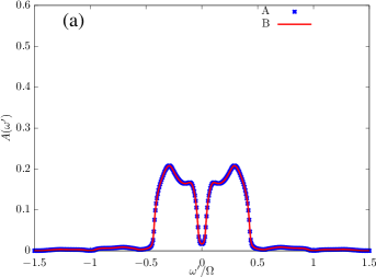
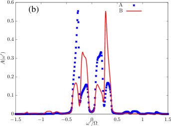
Figure 1: Spectral functions $A\left(\omega^{\prime}\right)=-\frac{1}{\pi}\mathrm{Im}G^{R}_{nn}\left(\omega\right)$ with $\omega^{\prime}=\omega+n\Omega$ for the case without staggered potential in (a), and the case with staggered potential $\Omega\sum_{l}\lambda_{l}n_{l}$ in (b). The unit of the spectral function is [TL^-2]. For both panels, the driving frequency $\Omega=7J$, $\frac{K}{\Omega}=1.28$, and $\Delta=0$. Bath parameters are $\Gamma=T=0.05J$.

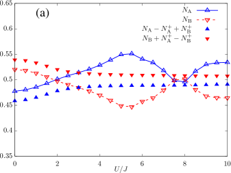
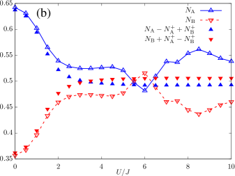
Figure 2: Charge density wave (CDW) for (a) $\Delta=-0.6J$ and (b) $\Delta=0$ versus interactions $U$ for a two-dimensional hexagonal optical lattice with $9\times 9$ unit cells and periodic boundary conditions in both $x$ and $y$ directions. For both panels, the driving frequency $\Omega=7J$ and $\frac{K}{\Omega}=1.28$. Bath parameters are $\Gamma=T=0.05J$. $N_{\mathrm{A}\left(\mathrm{B}\right)}^{+}$ is shown in Fig. 3.

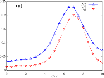
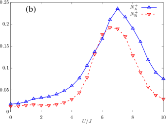
Figure 3: Charge density with positive frequency induced by resonant tunneling for (a) $\Delta=-0.6J$ and (b) $\Delta=0$, plotted versus interactions $U$. The peak is due to one-photon resonant tunneling when $U=\Omega$. Other parameters are the same as in Fig. 2.

There is a rich relation between charge density and interactions. We show the charge density $N_{\mathrm{A}\left(\mathrm{B}\right)}$ (lines with empty up triangle and empty down triangle) with increasing interactions in Fig. 2. (i) When $U=0$, the detuning $\Delta$ is the factor that affects occupation of A and B sites, and one can tune the occupations by changing $\Delta$. (ii) We next discuss the case where $0<U\apprle 3J$. The repulsive interaction $U$ counteracts the effect of $\Delta$, and the density difference is reduced. In this region, the resonant tunneling is suppressed because the bandwidth is smaller than the driving frequency. We show the spectral functions for $U=3J$ in Fig. 1(b), and we observe that the band width is approximately $\Omega$. The bandwidth is smaller than $\Omega$ for a smaller $U.$ (iii) When $U\apprge 3J$, resonant tunneling plays an important role. We define $N_{\mathrm{B}\left(\mathrm{A}\right)}^{+}=\frac{1}{2\pi}\int_{-\Omega/2}^{\Omega/2}d\omega\sum_{n,\omega+n\Omega>0}\mathrm{Im}G_{nn,\mathrm{B}\left(\mathrm{A}\right)}^{<}\left(\omega\right)$, which corresponds to the fraction of atoms occupying the upper Mott band. The reason for these excitations is the resonant tunneling induced by the hopping $\left\langle F\right|e^{i\tilde{\theta}_{\mathrm{B}\mathrm{A}}\left(t\right)}c_{\mathrm{B}}^{\dagger}c_{\mathrm{A}}\left|I\right\rangle$ between A and B sites in the correlated regime. If there were no such resonant tunneling, the fraction of atoms on A site would be estimated as $N_{\mathrm{A}}-N_{\mathrm{A}}^{+}+N_{\mathrm{B}}^{+}$, and similarly for B site it would be $N_{\mathrm{B}}+N_{\mathrm{A}}^{+}-N_{\mathrm{B}}^{+}$. If the estimation were accurate, we would have $N_{\mathrm{A}}-N_{\mathrm{A}}^{+}+N_{\mathrm{B}}^{+}\approx N_{\mathrm{B}}+N_{\mathrm{A}}^{+}-N_{\mathrm{B}}^{+}\approx 0.5$ for interactions $U\apprge 3$. As shown in Fig. 2(a) and (b), we note that both $N_{\mathrm{A}}-N_{\mathrm{A}}^{+}+N_{\mathrm{B}}^{+}$ (solid up triangle) and $N_{\mathrm{B}}+N_{\mathrm{A}}^{+}-N_{\mathrm{B}}^{+}$ (solid down triangle) are close to 0.5 when $U\apprge 3J$. This demonstrates that the resonant tunneling between A and B sites is the main contribution to the difference between the atom densities on A and B sites when $U$ is relatively large. This shows the characteristic difference between the NESS and an equilibrium state. On the other hand, it offers a way to estimate the resonant tunneling. Suppose it is possible to measure the charge density $N_{A}$ and $N_{B}$ for different interactions. One can then estimate the contribution of the resonant tunneling by calculating $N_{\mathrm{A}}-0.5$ or $0.5-N_{\mathrm{B}}$ for $U\apprge 3J$. (iii) There is some deviation from 0.5 for $N_{\mathrm{A}}-N_{\mathrm{A}}^{+}+N_{\mathrm{B}}^{+}$ and $N_{\mathrm{B}}+N_{\mathrm{A}}^{+}-N_{\mathrm{B}}^{+}$. It shows that there are high-order contributions, from the hopping A-B-A (or equivalently, B-A-B), to $N_{\mathrm{A}}^{+}$and $N_{\mathrm{B}}^{+}$. These contributions do not affect the number of atoms on A and B sites, but create excitations. This is also evidence for that the next-nearest neighbor hopping is effectively generated by lattice shaking, even though in this calculation we cannot show that it comes with a phase in this calculation.

We have a short comment regarding the case in Fig. 1(a). When the staggered potential is absent, there are still resonant tunnelings. However, they are the same for A and B sites, in contrast to the case with staggered potentials.

In Fig. 3, the charge density with positive frequency ($N_{\mathrm{A}\left(\mathrm{B}\right)}^{+}=\frac{1}{2\pi}\int_{-\Omega/2}^{\Omega/2}d\omega\sum_{n,\omega+n\Omega>0}\mathrm{Im}G_{nn,\mathrm{A}\left(\mathrm{B}\right)}^{<}\left(\omega\right)$) is shown. It is corresponding to the effect of resonant tunneling Qin and Hofstetter (2018). The peak is at $U=\Omega=7J$, where the one-photon resonant tunneling is dominant. As we have discussed above, the contribution $N_{\mathrm{A}}^{+}$ ($N_{\mathrm{B}}^{\dagger}$) is due to the direct hopping from B (A) sites, plus higher-order contributions from A (B) sites. Generally, $N_{\mathrm{A}}^{+}>N_{\mathrm{B}}^{+}$, and atoms prefer to hop to A sites due to the higher staggered potential on B sites.

III.2 Edge states

In this section, we present topological properties of a circularly shaken hexagonal optical lattice. We investigate edge states in a cylinder geometry of a hexagonal optical lattice, with a flux $\Phi$ insertion (Fig. 4) Wang et al. (2014); Grushin et al. (2015); Zaletel et al. (2014). This is the setup in the Laughlin gedanken experiment Laughlin (1981). The insertion of flux is equivalent to a twisted boundary condition in the direction with periodic boundary condition Niu et al. (1985); Qi et al. (2006). It is a general setup with the potential to be generalized to disordered cases Qi et al. (2006).

With insertion of one flux quantum, we demonstrate the change of topological properties of the system. Edge states are hallmarks of nontrivial topological properties. Using real-space Floquet DMFT, we study the interplay between interactions and edge states. We show the spectral functions in Fig. 5. For finite detuning $\Delta$, the cylinder geometry can host edge states (lines around $\omega^{\prime}=0$ in Fig. 5(a)) when $U=0$. With increasing interactions, the edge states as a function of the inserted flux $\Phi$ are smeared out as can be seen in Fig. 5(b)-(d). This corresponds to a finite lifetime of quasiparticles. The sharp spectral peak of a quasiparticle is gradually expanded due to increasing interactions. When $U=3J$, we see a simple Mott gap (Fig. 5(f)). We observe three different phases: Chern insulator with edge states present, pseudogap metallic phase with gap closed, and Mott insulator with gap open again. According to the effective Hamiltonian Tarnowski et al. (2017), the ratio between the next-nearest neighbor hopping $t_{2}$ and nearest neighbor hopping $t_{1}$ is $|t_{2}/t_{1}|=0.1$ with $|t_{1}|=0.5J$. The pseudogap metallic phase exists approximately when $U\approx 2J$. This is consistent with DMFT calculations in Ref. Nguyen and Tran (2013) for the Haldane-Falicov-Kimball model. The difference is that here we are considering a non-equilibrium driven system connected to a bath. The largest interaction $U=3J$ we have shown is much smaller than driving frequency $\Omega=7J$. It can therefore be expected that resonant tunneling is greatly suppressed. The dissipation rate $\Gamma$ into the bath has effects on the spectral functions especially for small $U$. It introduces an $i\Gamma$ correction to the self-energy and this term is equivalent to an interaction effect.

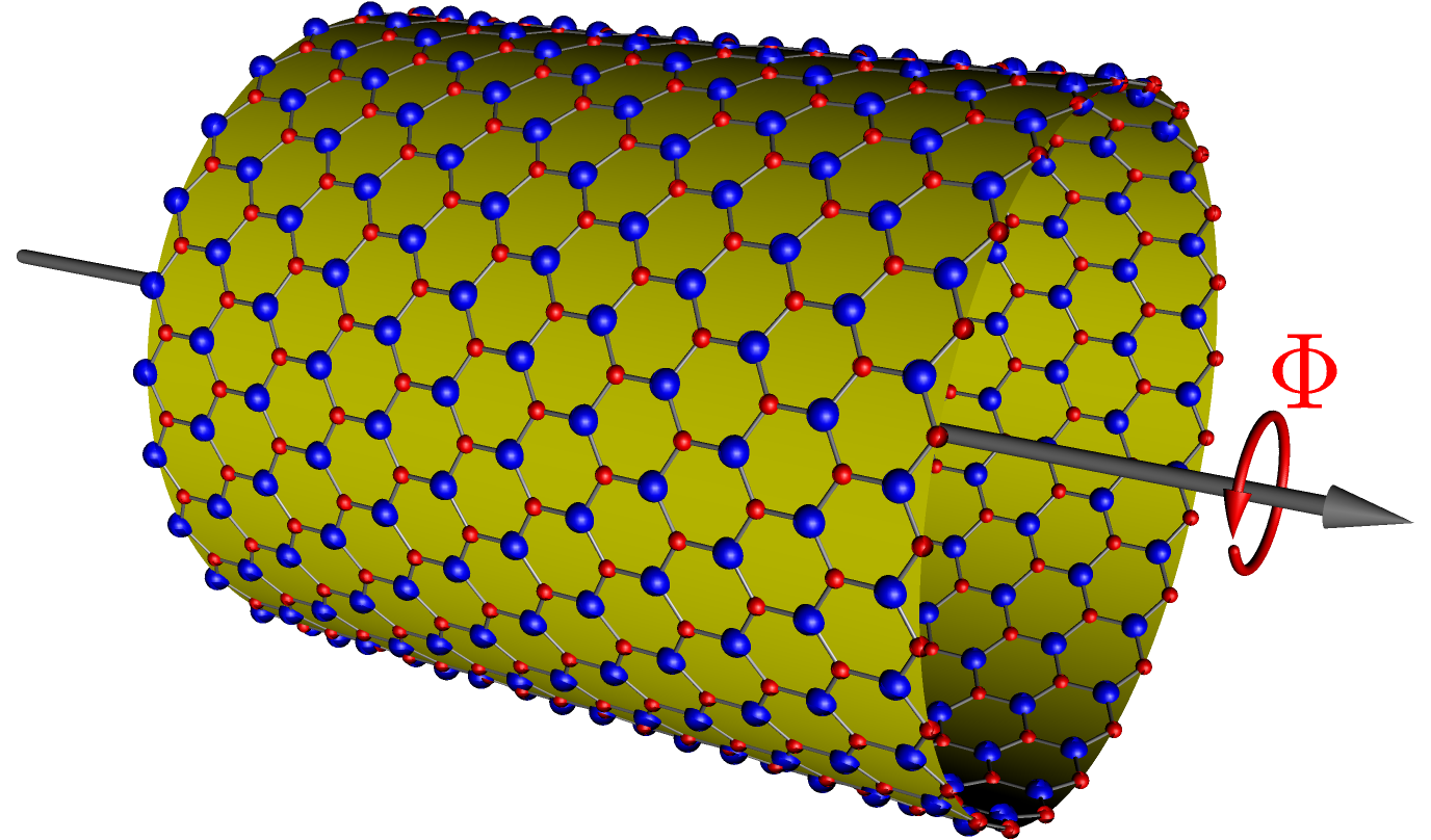
Figure 4: A cylinder geometry of a circularly shaken hexagonal optical lattice consisting of A (big blue sphere) and B (small red sphere) atoms with a flux $\Phi$ insertion. This is the setup in the Laughlin gedanken experiment Laughlin (1981). The zigzag boundary condition is used in the calculation. When there are well-defined edge states, they are expected to be present in the left and the right edges.

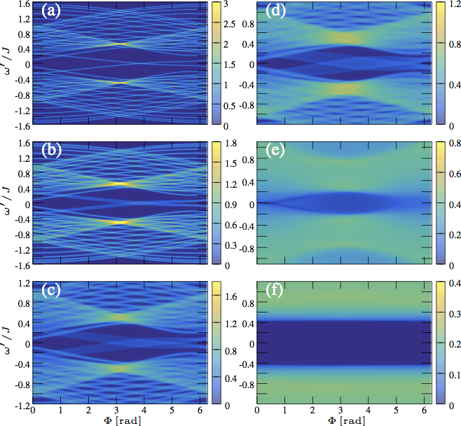
Figure 5: Spectral functions (with unit [TL^-2]) versus the flux $\Phi$ for different interactions. Explicitly, (a) $U=0$, (b) $U=0.1J$, (c) $U=0.2J$, (d) $U=0.3J$, (e) $U=0.7J$, and (f) $U=3J$. It shows interaction effects on edge states in a cylinder geometry of $3\times 10$ unit cells with $3$ unit cells in the direction with a periodical boundary condition. Other parameters are $\Omega=7J$, $\frac{K}{\Omega}=1.28$, and $\Delta=-0.35J$. Bath parameters are $\Gamma=0.005J$ and $T=0.01J$. $\omega^{\prime}$ indicates a general frequency which can be outside the first Brillouin zone of $\Omega$.

III.3 Charge pump

A second topological quantity which can be investigated in Laughlin’s setup is the charge pump, which is closely related to edge states. For an equilibrium system, when well-defined edge states are present in the cylinder geometry of a hexagonal optical lattice, a change of one flux quantum will induce an integer number of atoms to transfer from one edge of the cylinder to the other Laughlin (1981). The number of transferred atoms depends on the number of edge states. An integer charge pump is a signature of non-trivial topological phase. Following Ref. Wang et al. (2014), we define the charge pump with insertion of flux $\Phi$ as

$$Q_{\Phi}=Q_{\mathcal{R},\Phi}-Q_{\mathcal{L},\Phi}$$ (19)

which is the charge density difference between two halves of the cylinder (see Fig. 6: left (shading) and right (unshading) halves of the cylinder). $Q_{\alpha,\Phi}=\frac{1}{2\pi}\int_{-\Omega/2}^{\Omega/2}d\omega\sum_{i\in\alpha,n}\mathrm{Im}G_{i,\Phi,nn}^{<}\left(\omega\right)$ with $\alpha=\mathcal{R},\mathcal{L}$, and Floquet index $n$. $\mathrm{Im}G_{i,\Phi,nn}^{<}\left(\omega\right)=\frac{1}{2}\mathrm{Im}\left[G_{i,\Phi,nn}^{K}\left(\omega\right)-G_{i,\Phi,nn}^{R}\left(\omega\right)+G_{i,\Phi,nn}^{A}\left(\omega\right)\right]$, where $i$ is the site index in the left or right half. The flux is implemented according to Ref. Zaletel et al. (2014). Using the sum rule $-\frac{1}{\pi}\int_{-\Omega/2}^{\Omega/2}d\omega\mathrm{Im}\sum_{n}G_{i,\Phi,nn}^{R(A)}=1(-1)$, we have

$$Q_{\Phi}=\int_{-\Omega/2}^{\Omega/2}d\omega\sum_{n}\frac{1}{2\pi}\mathrm{Im}\left[G_{\mathcal{R},\Phi,nn}^{K}\left(\omega\right)-G_{\mathcal{L},\Phi,nn}^{K}\left(\omega\right)\right].$$ (20)

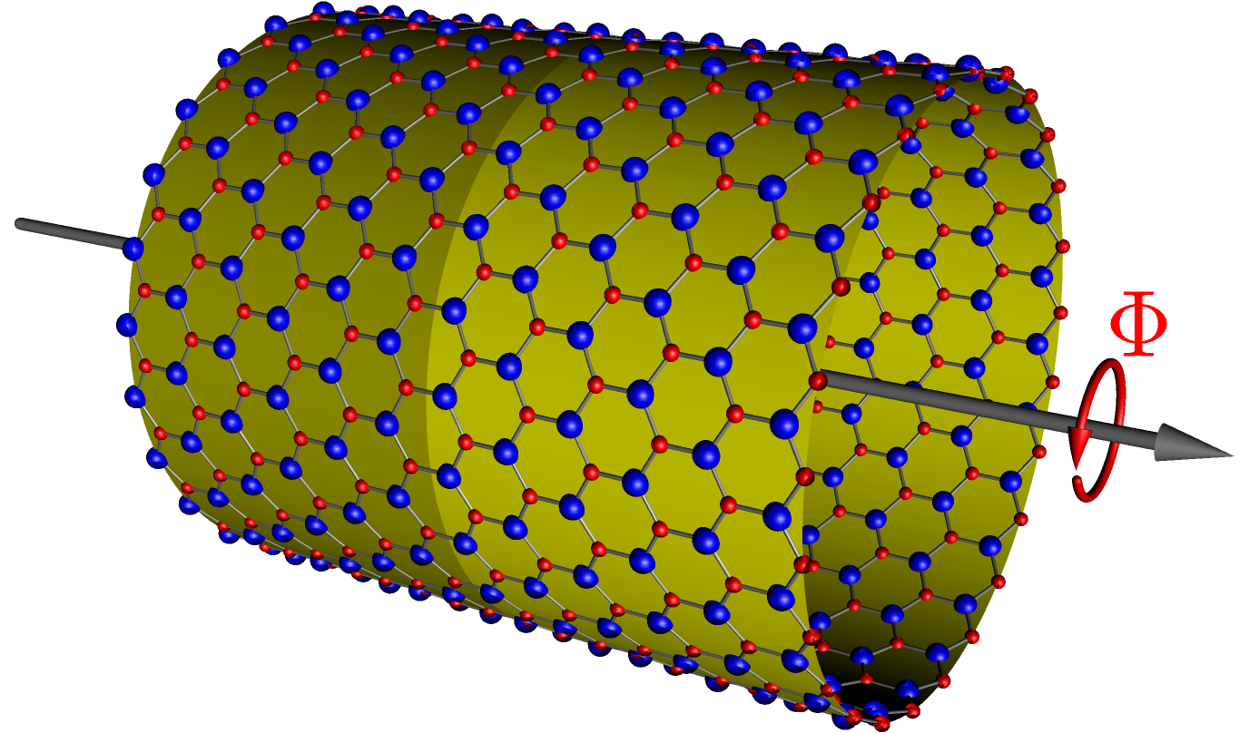
Figure 6: The charge pump with insertion of a flux $\Phi$ is defined as charge density difference $Q_{\Phi}=Q_{\mathcal{R},\Phi}-Q_{\mathcal{L},\Phi}$ between the two halves of the cylinder, as indicated by different background colors (shading and unshading).

III.3.1 An isolated equilibrium system

We show that $Q$ can indeed be a topological invariant to distinguish non-trivial and trivial topological phases for an non-interacting equilibrium state. For this case, no bath is needed for energy dissipation. We can determine the Keldysh Green’s function using the fluctuation-dissipation theorem Rammer (2007): $G^{K}\left(\omega\right)=\tanh\frac{\beta_{0}\omega}{2}\left(G^{R}\left(\omega\right)-G^{A}\left(\omega\right)\right)$, where $\beta_{0}=\frac{1}{k_{B}T_{0}}$ with $T_{0}$ the equilibrium temperature of the system. We choose $T_{0}$ as a very small number close to 0. The charge pump can be calculated as:

$$Q_{\Phi}= -\frac{1}{\pi}\mathrm{Im}\int_{-\Omega/2}^{\Omega/2}d\omega\sum_{n}f\left(\omega+n\Omega\right)$$

$$\times\mathrm{Im}\left[G_{\mathcal{R},\Phi,nn}^{R}\left(\omega\right)-G_{\mathcal{L},\Phi,nn}^{R}\left(\omega\right)\right].$$ (21)

$Q_{\Phi}$ can be calculated directly or using the technique of the contour integral. In Fig. 7, we show the charge pump versus flux insertion $\Phi$ for topologically non-trivial and trivial cases. In Fig. 7(a), we observe a sharp jump of the charge density difference $Q$ at the point $\Phi$, where two edge states intersect each other. It means that one atom is transferred from one edge of the cylinder to the other. In contrast, in the topologically trivial case (Fig. 7(b)), we only observe a smooth change in the charge density. Therefore, $Q_{\Phi}$ can serve as a topological invariant for distinguishing topologically non-trivial and trivial cases.

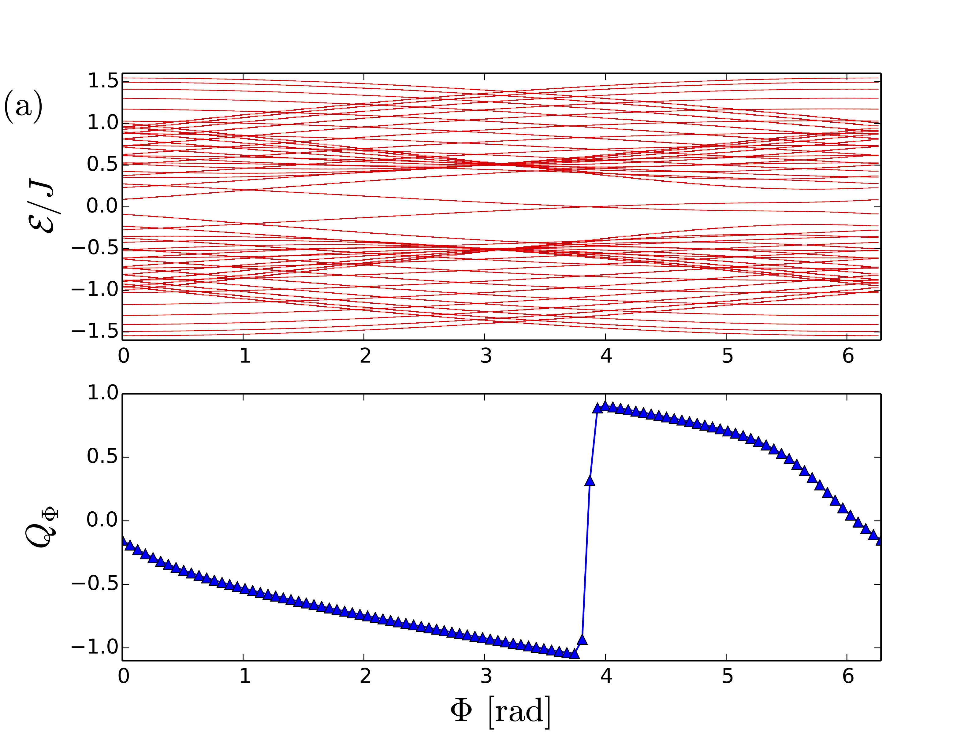
Figure 7: Energy spectrum $\mathcal{E}$ and charge pump $Q_{\Phi}$ with insertion of a flux for a cylinder hexagonal lattice with $3\times 10$ unit cells in an non-interacting equilibrium state. There are 3 unit cells in the direction with periodic boundary conditions. Other parameters are $\Omega=7J$, $\frac{K}{\Omega}=1.28$, $\Delta=-0.35J$ (panel (a)), and $\Delta=0.35J$ (panel (b)).

III.3.2 System coupled to a free fermion bath

We present the charge pump $Q$ for a NESS obtained from the real-space Floquet DMFT in Fig. 8. Corresponding to edge states in Fig. 5, we show that there is a jump in the charge pump in Fig. 8. However, the jump is not an integer even for very small interactions. With increasing interactions, the jump becomes very smooth. We explain why the jump is not integer even for $U=0$ (line with solid down triangle). It does not contradict to what we show in Fig. 7. In real-space Floquet DMFT, there is a bath coupled to every lattice site. With the approximation of constant DOS of the bath, the dissipation into the bath introduces a finite self-energy to the system. This is equivalent to an interaction effect. In fact, it is this effective interaction which destroys the integer charge pump when $U=0$. When the system couples to the environment (the bath) and becomes open, the unavoidable dissipation plays a role in the topological properties. Even though the dissipation is rather small, the interaction effect induced by it can be pronounced because the effective hopping is heavily dressed by the driving.

A connection can be made between the charge pump and CDW in Sec. III.1 Grusdt and Höning (2014). We observe a jump in both Figs. 8 and 9 for $U=0$, which signals a possible relationship. For the cylinder geometry threaded by flux, we can describe the CDW $Q_{\mathrm{A}}-Q_{\mathrm{B}}=Q_{\mathcal{R},\mathrm{A}}+Q_{\mathcal{L},\mathrm{A}}-Q_{\mathcal{R},\mathrm{B}}-Q_{\mathcal{L},\mathrm{B}}$, which is the total density difference between site A and B. The charge pump is defined by $Q_{\mathcal{R}}-Q_{\mathcal{L}}=Q_{\mathcal{R},\mathrm{A}}+Q_{\mathcal{R},\mathrm{B}}-Q_{\mathcal{L},\mathrm{A}}-Q_{\mathcal{L},\mathrm{B}}$. A simple comparison shows that the difference lies in the part $Q_{\mathcal{L},\mathrm{A}}-Q_{\mathcal{R},\mathrm{B}}$. In Fig. 9 we note that charge density difference between A and B exists at $\Phi=0$ due to CDW, and we see a clear jump when $\Phi\approx 3.8\mathrm{[rad]}$ for $U=0$ (line with solid down triangle), exactly where the jump happens for the charge pump in Fig. 8. For the equilibrium case, see Ref. Sup . Therefore, for a pronounced charge pump, there must be a dominated hopping process from A to B or from B to A, which can lead to a significant density redistribution between A and B. Furthermore, our discussion in Sec. III.1 shows that the weak interaction counteracts the effects of staggered potentials, and makes the density difference between A and B smaller. Consistently, in Fig. 9 we see that changes in charge density difference versus $\Phi$ becomes smaller with increasing interactions.

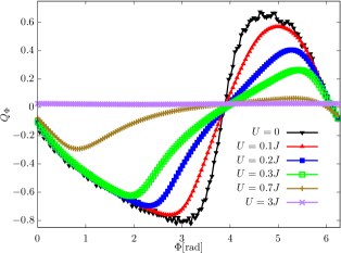
Figure 8: Charge pump $Q_{\Phi}$ with insertion of a flux $\Phi$ for a cylinder hexagonal lattice, obtained by real-space Floquet DMFT for different interactions. The parameters are the same as those in Fig. 5. For the non-interacting case, we obtain the charge pump by a direct calculation of the non-interacting Floquet Green’s function with the bath corrections. It is different from the method of rate equations in Sec. III.3.3.

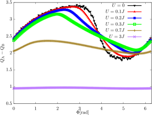
Figure 9: The total charge density difference $Q_{A}-Q_{B}$ on a cylinder hexagonal lattice for the (interacting) Floquet case coupled to a bath. The parameters are the same as those in Fig. 5. A jump is observed for $U=0$ (line with solid down triangle).

III.3.3 System coupled to a heat bath

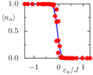
(a)

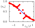
(b)

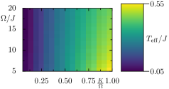
(c)

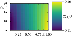
(d)

Figure 10: NESS that forms when the system is coupled to an ohmic heat bath (no cutoff, $E_{c}=\infty$) at $T=0.001J$. (a, b) We obtain effective temperatures by fitting the distribution $\langle n_{a}\rangle$ (red dots) of the NESS with a Fermi-Dirac distribution with temperature $T_{\mathrm{eff}}$ (blue solid line), where (a) $\Delta=-0.1J$, $\Omega=5J$, $K/\Omega=0.05$ and (b) $\Delta=-0.3J$, $\Omega=13.33J$, $K/\Omega=1$. (c, d) $T_{\mathrm{eff}}$ as a function of driving parameters, for (c) $\Delta=-0.1J$ and (d) $\Delta=-0.3J$. We show states for a $3\times 7$ lattice, but we observe that $T_{\mathrm{eff}}$ is almost independent of the size of the lattice.

To further identify the role of dissipation to the bath in the charge pump for a non-interacting system, we here study the NESS that forms when the driven system at half filling is coupled to an ohmic heat bath, using the rate equations.

Similar to the fermionic reservoir, we couple one heat bath at temperature $T$ to every site of the lattice. This is mediated by a coupling operator $v_{(l)}=c^{\dagger}_{l}c_{l}$ for a given site $l$. Note that we assume this form of the coupling for the direct frame. However, if we transform the coupling to the co-moving frame, it still obeys the same form since the unitary rotation $\mathcal{U}$ commutes with the coupling $c^{\dagger}_{l}c_{l}$. From Eq. (14) one then infers rates $R^{(l)}_{ab}$ that result from coupling this site $l$ to the heat bath. The total rates for coupling the system globally to an external heat bath result from the incoherent sum of all of these processes, implying $R_{ab}=\sum_{l}R^{(l)}_{ab}$.

With these rates we solve the kinetic equation (18) for the NESS. Just to remind the reader, the resulting state is the long-time steady state that results when the system is under a constant driving and weakly coupled to the bath, meaning that the coupling constant is small when compared to all quasi-energy splittings in the system, $\sqrt{\Gamma}\ll(\varepsilon_{k}-\varepsilon_{q})$, for $k\neq q$.

We observe that for frequencies $\Omega$ which are large when compared to the bandwidth, the distributions $\langle n_{a}\rangle$ that we observe in the NESS are still close to thermal distributions with an effective temperature $T_{\mathrm{eff}}$, cf. the examples in Fig. 10(a) and (b). This effective temperature is obtained by fitting the closest thermal distribution to the occupations such that $\langle n_{a}\rangle\approx 1/(\mathrm{e}^{(\varepsilon_{a}-\mu)/T_{\mathrm{eff}}}+1)$, and therefore assuming what was called a “Floquet-Gibbs” state in the literature Shirai et al. (2016). Note that in Fig. 10, the temperature of the bath is $T=0.001J$, but still, due to the driving, in the long-time limit the system heats up to quite high temperatures that are on the order of $T_{\mathrm{eff}}\approx 0.1J$ as shown in Fig. 10(c) and (d) for a heat bath with ohmic spectral density and no spectral cutoff, $J(E)\propto E$. Interestingly, in this frequency regime, the effective temperature of the steady state seems to depend only on the relative strength $K/\Omega$ of the driving. Note that this is in contrast to the analytic formula that was presented in Ref. Iadecola et al. (2015), where in addition to the $K/\Omega$ dependence they find a term that scales as $1/\Omega^{d}$ (where $d$ is the exponent of the spectral density). In our calculations we also observe that $T_{\mathrm{eff}}$ is practically independent of the size of the lattice.

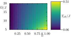
(a)

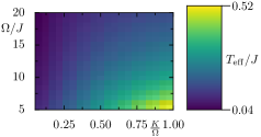
(b)

Figure 11: As in Figure 10(d), but (a) with $J(E)\propto E^{0.5}$ and (b) with $J(E)\propto E\exp(-E/5J)$.

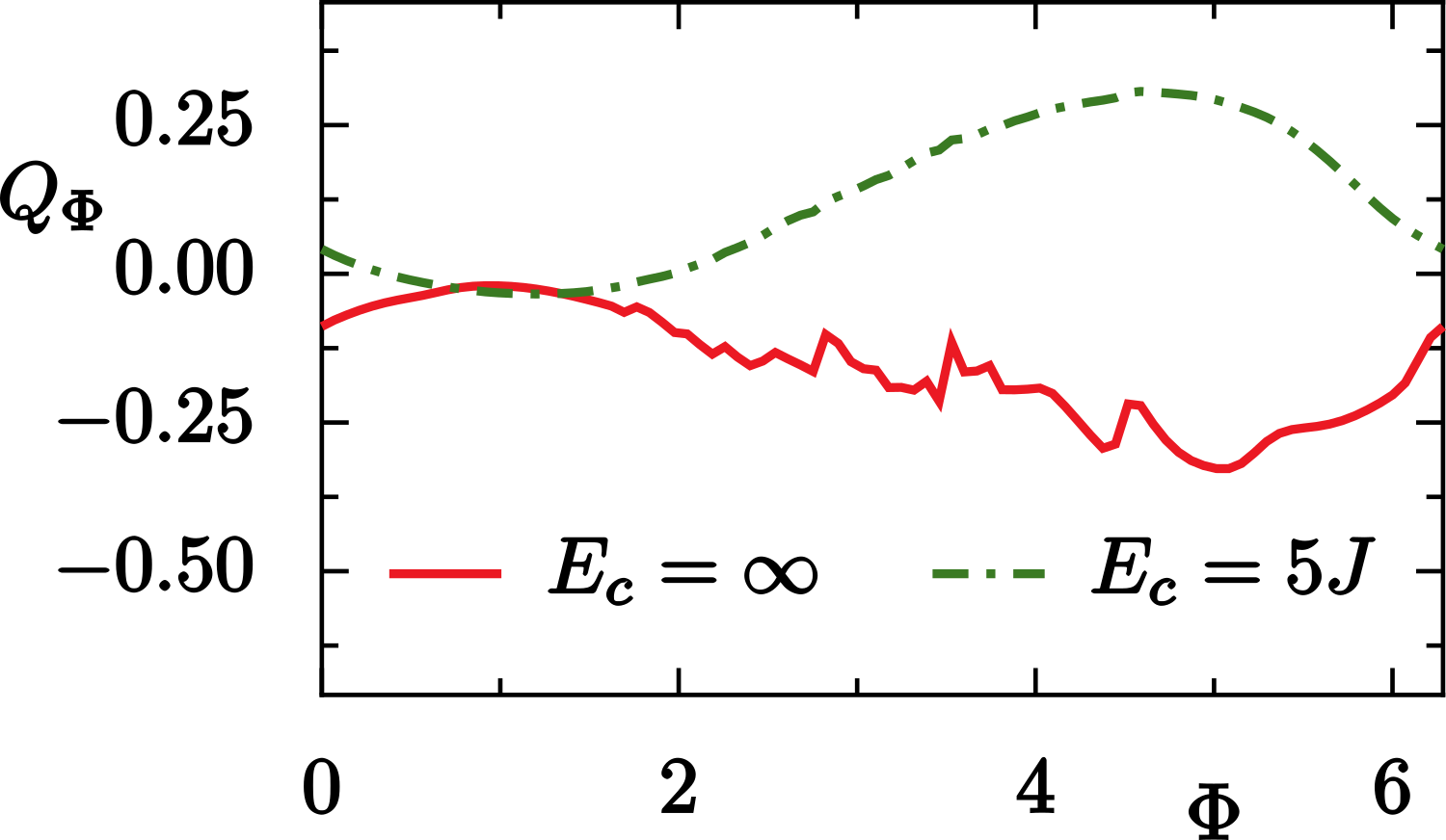
(a)

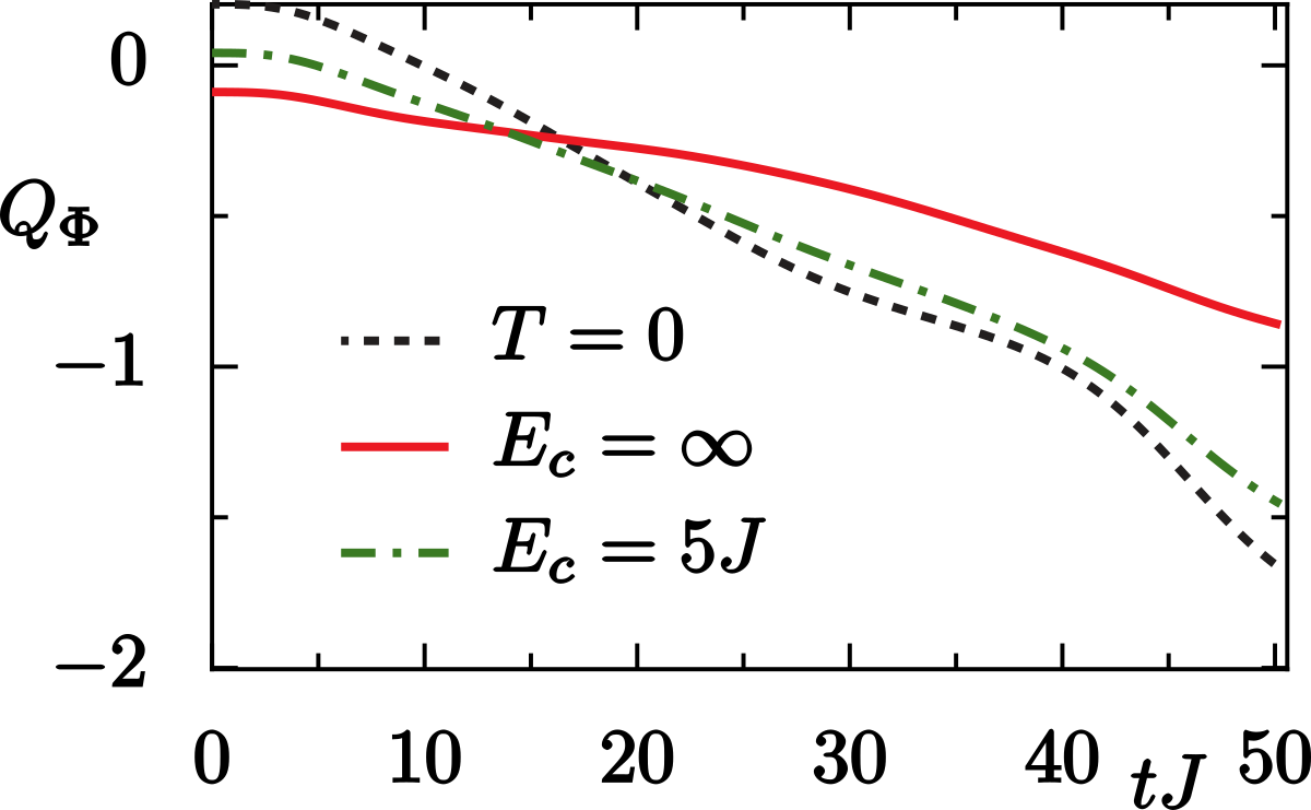
(b)

Figure 12: (a) Charge Pump $Q_{\Phi}$ with insertion of a flux $\Phi$ for parameters $\Omega=20J,\Delta=-0.1J,K/\Omega=0.25$ in a $3\times 10$ lattice where we expect the system to be topological. For given flux $\Phi$ we let the system relax to the NESS in presence of a heat bath with $J(E)\propto E\exp(-E/E_{c})$ and $T=0.001J$. For the green dash-dotted curve there is a spectral cutoff $E_{c}=5J$, the red solid curve is for ohmic bath. Using this procedure the signal is very weak, even though the effective temperature in the NESS are quite low. (b) However, there is a large transport signal if we prepare the NESS at $\Phi=0$ and then ramp (at constant speed) one flux quantum within a finite ramp time $\tau\approx 50/J$. Here, the red solid and green dash-dotted lines show snapshots of the system at integer multiples of $\mathcal{T}$ neglecting the micromotion. The green dash-dotted line (with some cutoff in the spectral density) features a relatively large charge transport that is close to the (almost) integer transport behavior that we expect for hypothetic thermal $T=0$ populations of the quasienergies (black dashed line).

Even by further decreasing the temperature $T$ of the bath, we are not able to reach lower effective temperatures $T_{\mathrm{eff}}$. We checked this by comparing to the NESS for a hypothetic $T=0$ bath, where there are no bath occupations $n_{B}=0$, so that there is only spontaneous emission. These relatively large effective temperatures are detrimental for the observation of quantized charge pumping, since they correspond to a significant occupation of the “upper” Floquet band. An extremely low temperature is vital for the exactness of the integer quantum Hall effect Giuliani and Vignale (2005). A finite temperature excites the particles across the gap, while a low temperature can make this probability exponentially low.

Note that this heating is due to the population transfer between Floquet states that is induced due to the presence of the coupling to the higher Floquet sidebands. As was pointed out in the literature Seetharam et al. (2015); Iadecola et al. (2015); Dehghani et al. (2015), this heating can be suppressed by engineering the bath such that the spectral density $J(E)$ at large quasi-energy differences becomes smaller. For example if we suppose the bath is sub-ohmic with $J(E)\propto E^{0.5}$, as shown in Fig. 11(a), then at large frequencies $\Omega$ we find that heating is suppressed, leading to lower effective temperatures $T_{\mathrm{eff}}$ in the NESS. Similar suppression of heating is found in Fig. 11(b) for an ohmic bath, but with a finite cutoff $E_{c}=5J$ in the spectral density $J(E)\propto E\exp(-E/E_{c})$. Note that it has been argued in the literature that in the limit $\Omega\gg E_{c}$ resonances are suppressed and one expects an effectively thermalized “Floquet-Gibbs” state Shirai et al. (2016). Such a finite frequency cutoff is the manifestation of bath correlation times $\tau_{R}\propto 1/E_{c}$ that are on the order of the time scales of the system dynamics $\tau_{S}\propto 1/J$. Note that such finite correlation times are tunable e.g. in the case where the bath is a weakly interacting Bose-Einstein condensate in a trap. There, excitations are nicely described by Bogoliubov quasiparticles (phonons) Ozeri et al. (2005) and the bath correlation times can be controlled by the trap frequency Klein and Fleischhauer (2005); Ostmann and Strunz (2017). Also, sympathetic cooling of fermions in Bose-Einstein condensates is a well established experimental technique, however there, typically a relatively strong coupling $\Gamma$ is favorable, while here we target weak couplings.

If we now use a NESS that was prepared in presence of such a heat bath, one again may ask whether one can observe the underlying topological nature of the model. Similar to the DMFT calculations in presence of the fermionic reservoir, in Fig. 12(a) we show the charge difference $Q_{\Phi}$ of the right and lefthand side of the system in the NESS that was prepared for a given value of the flux $\Phi$. However, even though for these parameters the model is topological and the effective temperatures are relatively low, especially in the case with a finite cutoff in the spectral density (green dash-dotted line), we do not see a pronounced peak in the charge difference.

In order to overcome this problem, we propose a different strategy to probe topology in the model. Namely, in Fig. 12(a) it is assumed that the ramp time $\tau$ is big when compared to the relaxation times $\tau_{R}$, i.e. we follow the system adiabatically in the thermodynamic sense. Here, since we are in the weak coupling regime where $\tau_{R}$ is large, we propose to perform a ramp on a much shorter time scale $\tau\ll\tau_{R}$, such that during the ramp one may neglect the action of the bath. However, this ramp should still be slow when compared to system time scales $\tau_{s}\ll\tau$, which one might call adiabatic in the closed system (without the presence of the bath). The red solid and green dash-dotted lines in Fig. 12(b) show the charge transport that one observes in such a procedure, where we start with a NESS that is prepared without the presence of an external field, $\Phi_{\mathrm{NESS}}=0$. There, the values are quite high, for the ohmic bath with a cutoff. The density difference between two halves of the cylinder $Q_{\Phi}$ is up to about 1.4 (green dash-dotted line), corresponding to $0.7$ of a charge is transported, which is very close to the quantized value that we expect for such a ramp if we assume a $T=0$ population of the quasi-energies (black dashed line).

III.4 Experimental relevance

We discuss the possibilities to observe the physical quantities we have explored in an experiment. To detect the CDW, one can measure the local densities on A and B sites either in situ in a quantum gas microscope, after time of flight via adiabatic band mapping techniques, or via the double occupancy Messer et al. (2015). For the charge pump, one needs to compare the local particle density between two parts of the cylinder geometry. The extra flux, in fact, relaxes the requirement to have a periodic boundary condition in one direction. For a hexagonal lattice which is finite in both directions, if it is possible to connect the sites at the ends of one direction with a complex long-range hopping, we can realize this cylinder geometry with a flux. This might be easier using a synthetic dimension Boada et al. (2015). A second possible way is discussed in Ref. Łącki et al. (2016). It proposes to use Laguerre-Gauss beams to create a cylinder optical lattice. Another possibility is to engineer a ring shaped system with the central hole pierced by a tunable magnetic flux, as it can be realized using the scheme proposed in Ref. Wang et al. (2018). For the charge pump measurement, as we have shown for the non-interacting case with rate equations, there is the possibility to couple the system weakly to a low-temperature heat bath to prepare the system in a state close to equilibrium. Bath engineering can be used to reach sufficiently low effective temperatures in the NESS. Then, the flux can be adiabatically ramped up to have a pronounced charge pump.

The Falicov-Kimball interaction can be realized in different possible ways Eckstein (2009); Jotzu et al. (2015). By introducing two species of atoms to the optical lattice, one species of atoms can be localized by a deep optical lattice depth Eckstein (2009). The localized atoms are in annealed disorder state for the Falicov-Kimball model, in contrast to the quenched disorder realized in ultracold atoms. It may be possible to be realized by switching off the hopping of the localized atoms slowly. A second possibility is presented in Ref. Jotzu et al. (2015) where the hopping of one species can be turnt off by tuning the driving amplitude because different species experience different driving amplitudes.

We have a comment on the bath. To study NESS in a driven system, it is necessary to connect the system to a bath to dissipate the extra energy. Most setups for cold atoms in optical lattices are isolated systems, but they can be in the prethermal regime when the driving frequency is sufficiently large. We may expect that the NESS in our setup may share some similarities for an isolated system in the prethermal regime Else et al. (2017); Kuwahara et al. (2016); Mori et al. (2016).

IV Conclusion

In conclusion, we have studied the charge density wave and charge pump of fermions with Falicov-Kimball interactions in a circularly shaken hexagonal optical lattice. We show that the charge density wave is induced by the staggered potential and is dramatically changed because of resonant tunneling. We also show interaction effects on the topological properties. An increase of the Falicov-Kimball interaction tends to smear out the edge states, and finally makes the system enter the Mott insulator phase.

Furthermore, we study non-equilibrium steady states in a Laughlin charge pump setup which is coupled to either a fermionic reservoir or a heat bath. In the interacting case, we show that the charge pump is not integer for insertion of one flux quantum. Also for the non-interacting case, we find that it is not integer due to dissipation into a bath. We confirm this by detailed calculations via rate equations based on the Floquet-Born-Markov approximation. Moreover, we explored possibilities to lower the effective temperature characterizing the NESS of the driven system by engineering the spectral properties of the bath. Our calculations suggest that in theory one can indeed use the presence of a bath to cool down the system, e.g. after a quench where in the closed system typically there are excitations in the upper band, and also to some extent one can overcome the heating that is inherent in the interacting Floquet system. We propose an experimentally feasible procedure to ramp up the flux for the measurement of the charge pump.

In the future, the approaches developed here can also be applied to the Haldane-Hubbard model, where both spin states are mobile, and which is naturally realized with cold atoms in optical lattices.

V Acknowledgments

This work is supported by the Deutsche Forschungsgemeinschaft via DFG FOR 2414 and the high-performance computing center LOEWE-CSC. The authors acknowledge useful discussions and communication with M. Eckstein, K. Le Hur, and N. Tsuji.

Supplementary material

V.1 Impurity solver for the Falicov-Kimball model

We outline how to include the Falicov-Kimball interaction in the impurity part following Refs. Eckstein and Kollar (2008) and (Eckstein, 2009, chapter 5.2) in the formalism of nonequilibrium DMFT.

1. In DMFT, for a given site, local correlation functions are obtained from an effective single-site problem with action

   $$\mathcal{S}= \mathcal{S}_{\mathrm{loc}}+\mathcal{S}_{\mathrm{hyb}}$$ (S1)

   $$\mathcal{S}_{\mathrm{loc}}= -i\int_{\mathcal{C}}dtH_{\mathrm{loc}}\left(t\right)-i\mu\sum_{\sigma}\int_{\mathcal{C}}dtc_{\sigma}^{\dagger}\left(t\right)c_{\sigma}\left(t\right)$$ (S2)

   $$\mathcal{S}_{\mathrm{hyb}}= -i\sum_{\sigma\sigma^{\prime}}\int_{\mathcal{C}}dt\int_{\mathcal{C}}dt^{\prime}c_{\sigma}^{\dagger}\left(t\right)\Lambda_{\sigma\sigma^{\prime}}\left(t,t^{\prime}\right)c_{\sigma^{\prime}}\left(t^{\prime}\right)$$ (S3)

   where $\mathcal{S}_{\mathrm{loc}}$ contains the dynamics induced due to the local Hamiltonian $H_{\mathrm{loc}}\left(t\right)=U\left(t\right)n_{\uparrow}\left(t\right)n_{\downarrow}\left(t\right)$. For the Falicov-Kimball interaction, one can imagine one spin species as the $f$-particle.

2. For the Falicov-Kimball model, in DMFT there is an important simplification for the action $\mathcal{S}$ due to the immobility of the $f$-particles: $\Lambda_{ff}\left(t,t^{\prime}\right)=0$. In fact, $\Lambda_{ff}\left(t,t^{\prime}\right)$ describes temporal fluctuations of the $f$-particle density. We can replace the density operator $f^{\dagger}\left(t\right)f\left(t\right)$ by the time independent operator $n_{f}$ in the action, and we have the local Green’s function for a general time-dependent interaction $U\left(t\right)$:

   $$G\left(t,t^{\prime}\right)= -i\frac{\mathrm{Tr}_{c,f}\left[e^{-\beta H_{0}}\mathrm{T}_{\mathcal{C}}\exp\left(\mathcal{S}\left[n_{f}\right]\right)c\left(t\right)c^{\dagger}\left(t^{\prime}\right)\right]}{\mathrm{Tr}_{c,f}\left[e^{-\beta H_{0}}\mathrm{T}_{\mathcal{C}}\exp\left(\mathcal{S}\left[n_{f}\right]\right)\right]}$$ (S4)

   $$\mathcal{S}\left[n_{f}\right]= -i\int_{\mathcal{C}}d\bar{t}\int_{\mathcal{C}}d\bar{t}^{\prime}c^{\dagger}\left(\bar{t}\right)\Lambda\left(\bar{t},\bar{t}^{\prime}\right)c\left(\bar{t}^{\prime}\right)-in_{f}\int_{\mathcal{C}}d\bar{t}U\left(\bar{t}\right)c^{\dagger}\left(\bar{t}\right)c\left(\bar{t}\right)+\left(E_{f}-\mu\right)n_{f}$$ (S5)

   where $H_{0}=\mu c^{\dagger}c$, $\mathrm{Tr}_{c,f}$ means trace over $c$ and $f$ degrees of freedom, and $\mathcal{C}$ denotes Keldysh contour. We introduce the definition

   $$Z_{n_{f}}=\mathrm{Tr}_{c}\left[e^{-\beta H_{0}}\mathrm{T}_{\mathcal{C}}\exp\left(\mathcal{S}\left[n_{f}\right]\right)\right]$$ (S6)

   with $n_{f}=0,1$. Tracing over the $f$ degrees of freedom, we have

   $$G\left(t,t^{\prime}\right)=w_{0}Q\left(t,t^{\prime}\right)+w_{1}R\left(t,t^{\prime}\right)$$ (S7)

   where

   $$Q\left(t,t^{\prime}\right)= -i\frac{\mathrm{Tr}_{c}\left[e^{-\beta H_{0}}\mathrm{T}_{\mathcal{C}}\mathcal{S}\left[0\right]c\left(t\right)c^{\dagger}\left(t^{\prime}\right)\right]}{Z_{0}},$$ (S8)

   $$R\left(t,t^{\prime}\right)= -i\frac{\mathrm{Tr}_{c}\left[e^{-\beta H_{0}}\mathrm{T}_{\mathcal{C}}\mathcal{S}\left[1\right]c\left(t\right)c^{\dagger}\left(t^{\prime}\right)\right]}{Z_{1}},$$ (S9)

   and

   $$w_{1}=1-w_{0}=\frac{Z_{1}}{Z_{0}+Z_{1}}$$ (S10)

   is in fact the definition for $f$-particle density (exactly in the sense of statistical average). Generally, $w_{1}$ depends on the $c$-particle configuration and $E_{f}$ by Eqs. (S6) and (S10) in a very complicated way and is not known a priori. We focus on the homogeneous phase of $f$-particles. For the half-filling we have investigated, we simply have $w_{1}=w_{0}=\frac{1}{2}$.

3. To obtain $Q\left(t,t^{\prime}\right)$ and $R\left(t,t^{\prime}\right)$, one can investigate them by equations of motion. Then we transform all the Green’s functions in Eq. (S7) into the Floquet space. Finally, we obtain Eq. (10) presented in the manuscript.

V.2 Charge pump and charge density wave for the equilibrium case

For the equilibrium case, we make a connection between charge pump and charge density wave (CDW) Grusdt and Höning (2014). As we argued in the main text, the difference between charge pump and CDW lies in the part $Q_{\mathcal{L},\mathrm{A}}-Q_{\mathcal{R},\mathrm{B}}$. We show in Fig. 1 the charge pump (Fig. 1.(a)) and CDW (Fig. 1.(b)) for a non-interacting, dissipationless and topologically non-trivial case. We observe a jump in both cases, which signals a possible relationship. For a pronounced integer charge pump, there must be a dominated process from A to B or from B to A, which leads to a significant density redistribution between A and B. As shown in Fig. 1.(d), the dominated process is from A to B when $\Phi\approx 3.8\mathrm{[rad]}$. It is because the density on A site is higher than that on B site (Fig. 1.(b)) due to CDW. Therefore, we can see that a significant CDW favors charge pump.

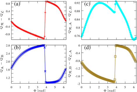
Figure 1: Charge pump $Q_{\mathcal{R}}-Q_{\mathcal{L}}$ and charge density wave $Q_{A}-Q_{B}$ for the non-interacting equilibrium and topological non-trivial case without dissipation. The parameters are the same as the panel (a) of Fig. 7 in the manuscript.

References

- Eckardt (2017) A. Eckardt, Rev. Mod. Phys. 89, 011004 (2017).
- Goldman et al. (2016) N. Goldman, J. C. Budich, and P. Zoller, Nat. Phys. 12, 639 (2016).
- Aidelsburger et al. (2013) M. Aidelsburger, M. Atala, M. Lohse, J. T. Barreiro, B. Paredes, and I. Bloch, Phys. Rev. Lett. 111, 185301 (2013).
- Miyake et al. (2013) H. Miyake, G. A. Siviloglou, C. J. Kennedy, W. C. Burton, and W. Ketterle, Phys. Rev. Lett. 111, 185302 (2013).
- Aidelsburger et al. (2015) M. Aidelsburger, M. Lohse, C. Schweizer, M. Atala, J. T. Barreiro, S. Nascimbene, N. R. Cooper, I. Bloch, and N. Goldman, Nat. Phys. 11, 162 (2015).
- Jotzu et al. (2014) G. Jotzu, M. Messer, R. Desbuquois, M. Lebrat, T. Uehlinger, D. Greif, and T. Esslinger, Nature 515, 237 (2014).
- Fläschner et al. (2016) N. Fläschner, B. S. Rem, M. Tarnowski, D. Vogel, D. S. Lühmann, K. Sengstock, and C. Weitenberg, Science 352, 1091 (2016).
- Fläschner et al. (2017) N. Fläschner, D. Vogel, M. Tarnowski, B. S. Rem, D. S. Lühmann, M. Heyl, J. C. Budich, L. Mathey, K. Sengstock, and C. Weitenberg, Nat. Phys. 14, 265 (2017).
- Lu et al. (2016) H.-I. Lu, M. Schemmer, L. M. Aycock, D. Genkina, S. Sugawa, and I. B. Spielman, Phys. Rev. Lett. 116, 200402 (2016).
- Lohse et al. (2016) M. Lohse, C. Schweizer, O. Zilberberg, M. Aidelsburger, and I. Bloch, Nat. Phys. 12, 350 (2016).
- Nakajima et al. (2016) S. Nakajima, T. Tomita, S. Taie, T. Ichinose, H. Ozawa, L. Wang, M. Troyer, and Y. Takahashi, Nat. Phys. 12, 296 (2016).
- Lohse et al. (2018) M. Lohse, C. Schweizer, H. M. Price, O. Zilberberg, and I. Bloch, Nature 553, 55 (2018).
- Hauke et al. (2014) P. Hauke, M. Lewenstein, and A. Eckardt, Phys. Rev. Lett. 113, 045303 (2014).
- Tarnowski et al. (2017) M. Tarnowski, F. N. Ünal, N. Fläschner, B. S. Rem, A. Eckardt, K. Sengstock, and C. Weitenberg, arXiv: 1709.01046 (2017).
- Wang et al. (2017) C. Wang, P. Zhang, X. Chen, J. Yu, and H. Zhai, Phys. Rev. Lett. 118, 185701 (2017).
- Bukov et al. (2015a) M. Bukov, L. D’Alessio, and A. Polkovnikov, Adv. Phys. 64, 139 (2015a).
- D’Alessio and Rigol (2014) L. D’Alessio and M. Rigol, Phys. Rev. X 4, 041048 (2014).
- Lazarides et al. (2014a) A. Lazarides, A. Das, and R. Moessner, Phys. Rev. E 90, 012110 (2014a).
- Ponte et al. (2015) P. Ponte, Z. Papić, F. m. c. Huveneers, and D. A. Abanin, Phys. Rev. Lett. 114, 140401 (2015).
- Lazarides et al. (2015) A. Lazarides, A. Das, and R. Moessner, Phys. Rev. Lett. 115, 030402 (2015).
- Lazarides et al. (2014b) A. Lazarides, A. Das, and R. Moessner, Phys. Rev. Lett. 112, 150401 (2014b).
- Bukov et al. (2015b) M. Bukov, S. Gopalakrishnan, M. Knap, and E. Demler, Phys. Rev. Lett. 115, 205301 (2015b).
- Weidinger and Knap (2017) S. A. Weidinger and M. Knap, Sci. Rep. 7, 45382 (2017).
- Weinberg et al. (2015) M. Weinberg, C. Ölschläger, C. Sträter, S. Prelle, A. Eckardt, K. Sengstock, and J. Simonet, Phys. Rev. A 92, 043621 (2015).
- Görg et al. (2018) F. Görg, M. Messer, K. Sandholzer, G. Jotzu, R. Desbuquois, and T. Esslinger, Nature 553, 481 (2018).
- Reitter et al. (2017) M. Reitter, J. Näger, K. Wintersperger, C. Sträter, I. Bloch, A. Eckardt, and U. Schneider, Phys. Rev. Lett. 119, 200402 (2017).
- Goldman and Dalibard (2014) N. Goldman and J. Dalibard, Phys. Rev. X 4, 031027 (2014).
- Eckardt and Anisimovas (2015) A. Eckardt and E. Anisimovas, New J. Phys. 17, 093039 (2015).
- Zheng et al. (2015) W. Zheng, H. Shen, Z. Wang, and H. Zhai, Phys. Rev. B 91, 161107 (2015).
- Plekhanov et al. (2017) K. Plekhanov, G. Roux, and K. Le Hur, Phys. Rev. B 95, 045102 (2017).
- Anisimovas et al. (2015) E. Anisimovas, G. Žlabys, B. M. Anderson, G. Juzeliūnas, and A. Eckardt, Phys. Rev. B 91, 245135 (2015).
- Bukov et al. (2016) M. Bukov, M. Kolodrubetz, and A. Polkovnikov, Phys. Rev. Lett. 116, 125301 (2016).
- Freericks et al. (2006) J. K. Freericks, V. M. Turkowski, and V. Zlatić, Phys. Rev. Lett. 97, 266408 (2006).
- Tsuji et al. (2008) N. Tsuji, T. Oka, and H. Aoki, Phys. Rev. B 78, 235124 (2008).
- Joura et al. (2008) A. V. Joura, J. K. Freericks, and T. Pruschke, Phys. Rev. Lett. 101, 196401 (2008).
- Freericks and Joura (2008) J. K. Freericks and A. V. Joura, “Nonequilibrium density of states and distribution functions for strongly correlated materials across the mott transition,” in Electron Transport in Nanosystems, edited by J. Bonča and S. Kruchinin (Springer Netherlands, Dordrecht, 2008) pp. 219–236.
- Aoki et al. (2014) H. Aoki, N. Tsuji, M. Eckstein, M. Kollar, T. Oka, and P. Werner, Rev. Mod. Phys. 86, 779 (2014).
- Laughlin (1981) R. B. Laughlin, Phys. Rev. B 23, 5632 (1981).
- Sohal and Eckardt (2016) R. Sohal and A. Eckardt, Draft (2016).
- Tsuji (2010) N. Tsuji, Theoretical Study of Nonequilibrium Correlated Fermions Driven by ac Fields, Ph.D. thesis, Department of Physics, University of Tokyo (2010).
- Qin and Hofstetter (2017) T. Qin and W. Hofstetter, Phys. Rev. B 96, 075134 (2017).
- Tsuji et al. (2009) N. Tsuji, T. Oka, and H. Aoki, Phys. Rev. Lett. 103, 047403 (2009).
- Rammer (2007) J. Rammer, Quantum Field Theory of Non-equilibrium States (Cambridge University Press, 2007).
- Brandt and Mielsch (1989) U. Brandt and C. Mielsch, Z. Phys. B Cond. Matt. 75, 365 (1989).
- Eckstein and Kollar (2008) M. Eckstein and M. Kollar, Phys. Rev. Lett. 100, 120404 (2008).
- (46) See supplementary material for details of the nonequilibrium impurity solver for the Falicov-Kimball model, and analysis on the relation between CDW and charge pump for equilibrium case.
- Breuer and Petruccione (2002) H. Breuer and F. Petruccione, The Theory of Open Quantum Systems (Oxford University Press, Oxford & New York, 2002).
- Kohler et al. (1998) S. Kohler, R. Utermann, P. Hänggi, and T. Dittrich, Phys. Rev. E 58, 7219 (1998).
- Hone et al. (2009) D. W. Hone, R. Ketzmerick, and W. Kohn, Phys. Rev. E 79, 051129 (2009).
- Cohen-Tannoudji (1994) C. Cohen-Tannoudji, Atoms in electromagnetic fields, Vol. 1 (World scientific, 1994).
- Vorberg et al. (2013) D. Vorberg, W. Wustmann, R. Ketzmerick, and A. Eckardt, Phys. Rev. Lett. 111, 240405 (2013).
- Vorberg et al. (2015) D. Vorberg, W. Wustmann, H. Schomerus, R. Ketzmerick, and A. Eckardt, Phys. Rev. E 92, 062119 (2015).
- Chen et al. (2003) L. Chen, J. K. Freericks, and B. A. Jones, Phys. Rev. B 68, 153102 (2003).
- Matveev et al. (2008) O. P. Matveev, A. M. Shvaika, and J. K. Freericks, Phys. Rev. B 77, 035102 (2008).
- Nguyen and Tran (2013) H.-S. Nguyen and M.-T. Tran, Phys. Rev. B 88, 165132 (2013).
- Qin and Hofstetter (2018) T. Qin and W. Hofstetter, Phys. Rev. B 97, 125115 (2018).
- Wang et al. (2014) L. Wang, H.-H. Hung, and M. Troyer, Phys. Rev. B 90, 205111 (2014).
- Grushin et al. (2015) A. G. Grushin, J. Motruk, M. P. Zaletel, and F. Pollmann, Phys. Rev. B 91, 035136 (2015).
- Zaletel et al. (2014) M. P. Zaletel, R. S. K. Mong, and F. Pollmann, J. Stat. Mech. Theory. Exp. 2014, P10007 (2014).
- Niu et al. (1985) Q. Niu, D. J. Thouless, and Y.-S. Wu, Phys. Rev. B 31, 3372 (1985).
- Qi et al. (2006) X.-L. Qi, Y.-S. Wu, and S.-C. Zhang, Phys. Rev. B 74, 045125 (2006).
- Grusdt and Höning (2014) F. Grusdt and M. Höning, Phys. Rev. A 90, 053623 (2014).
- Shirai et al. (2016) T. Shirai, J. Thingna, T. Mori, S. Denisov, P. Hänggi, and S. Miyashita, New J. Phys. 18, 053008 (2016).
- Iadecola et al. (2015) T. Iadecola, T. Neupert, and C. Chamon, Phys. Rev. B 91, 235133 (2015).
- Giuliani and Vignale (2005) G. Giuliani and G. Vignale, Quantum theory of the electron liquid (Cambridge University Press, 2005).
- Seetharam et al. (2015) K. I. Seetharam, C.-E. Bardyn, N. H. Lindner, M. S. Rudner, and G. Refael, Phys. Rev. X 5, 041050 (2015).
- Dehghani et al. (2015) H. Dehghani, T. Oka, and A. Mitra, Phys. Rev. B 91, 155422 (2015).
- Ozeri et al. (2005) R. Ozeri, N. Katz, J. Steinhauer, and N. Davidson, Rev. Mod. Phys. 77, 187 (2005).
- Klein and Fleischhauer (2005) A. Klein and M. Fleischhauer, Phys. Rev. A 71, 033605 (2005).
- Ostmann and Strunz (2017) P. Ostmann and W. T. Strunz, arXiv: 1707.05257 (2017).
- Messer et al. (2015) M. Messer, R. Desbuquois, T. Uehlinger, G. Jotzu, S. Huber, D. Greif, and T. Esslinger, Phys. Rev. Lett. 115, 115303 (2015).
- Boada et al. (2015) O. Boada, A. Celi, J. Rodríguez-Laguna, J. I. Latorre, and M. Lewenstein, New J. Phys. 17, 045007 (2015).
- Łącki et al. (2016) M. Łącki, H. Pichler, A. Sterdyniak, A. Lyras, V. E. Lembessis, O. Al-Dossary, J. C. Budich, and P. Zoller, Phys. Rev. A 93, 013604 (2016).
- Wang et al. (2018) B. Wang, F. N. Ünal, and A. Eckardt, arXiv: 1802.06815 (2018).
- Eckstein (2009) M. Eckstein, Nonequilibrium dynamical mean-field theory, Ph.D. thesis, University Augsburg (2009).
- Jotzu et al. (2015) G. Jotzu, M. Messer, F. Görg, D. Greif, R. Desbuquois, and T. Esslinger, Phys. Rev. Lett. 115, 073002 (2015).
- Else et al. (2017) D. V. Else, B. Bauer, and C. Nayak, Phys. Rev. X 7, 011026 (2017).
- Kuwahara et al. (2016) T. Kuwahara, T. Mori, and K. Saito, Ann. Phys. 367, 96 (2016).
- Mori et al. (2016) T. Mori, T. Kuwahara, and K. Saito, Phys. Rev. Lett. 116, 120401 (2016).

References

- Eckstein and Kollar (2008) M. Eckstein and M. Kollar, Phys. Rev. Lett. 100, 120404 (2008).
- Eckstein (2009) M. Eckstein, Nonequilibrium dynamical mean-field theory, Ph.D. thesis, University Augsburg (2009).
- Grusdt and Höning (2014) F. Grusdt and M. Höning, Phys. Rev. A 90, 053623 (2014).