Human-Guided Data Exploration

Abstract.

The outcome of the explorative data analysis (EDA) phase is vital for successful data analysis. EDA is more effective when the user interacts with the system used to carry out the exploration. In the recently proposed paradigm of iterative data mining the user controls the exploration by inputting knowledge in the form of patterns observed during the process. The system then shows the user views of the data that are maximally informative given the user’s current knowledge. Although this scheme is good at showing surprising views of the data to the user, there is a clear shortcoming: the user cannot steer the process. In many real cases we want to focus on investigating specific questions concerning the data. This paper presents the Human Guided Data Exploration framework, generalising previous research. This framework allows the user to incorporate existing knowledge into the exploration process, focus on exploring a subset of the data, and compare different complex hypotheses concerning relations in the data. The framework utilises a computationally efficient constrained randomisation scheme. To showcase the framework, we developed a free open-source tool, using which the empirical evaluation on real-world datasets was carried out. Our evaluation shows that the ability to focus on particular subsets and being able to compare hypotheses are important additions to the interactive iterative data mining process.

1. Introduction

Explorative data analysis (EDA) has a long history and an established position in the data analysis community, dating back to the 1970s (tukey:1977, ). Tools for visual EDA are designed to present data in such a way that humans can use their innate pattern recognition skills when exploring the data. Visual exploration of data becomes more powerful when the user can interact with the system used to explore the data; such systems have also been around for a long time (fisherkeller, ) and the issue of combining interactive visualisations and advanced data analysis methods still remains open (vismasterbook, ).

Some of the main goals of data exploration is to allow the user to gain insight into the data and discover new, interesting aspects of the data. The limitation of most traditional systems is, however, that they do not allow the user to incorporate his or her background knowledge into the data analysis workflow. Recently, a new paradigm for iterative data mining has been proposed (hanhijarvi:2009, ; debie:2011a, ; debie:2011b, ; debie2013, ), in which the user iteratively explores the data, inputting his or her knowledge in the form of patterns during exploration. The identified patterns are taken into account in the further iterative data exploration steps. The iterative data mining approach has also been successfully applied in visual EDA (puolamaki:2016, ; kang:2016b, ; puolamaki2017, ).

In the iterative data mining framework, the knowledge that the user has about the data is modelled through a probability distribution (the background distribution), over the datasets conforming to the user’s knowledge. As the user learns more about the data, new knowledge is incorporated as patterns that constrain the distribution of possible datasets. Initially it is assumed that the user has no knowledge of the data, in which case the starting distribution is uninformative, e.g., a maximum entropy distribution or an empirical distribution obtained by permutations. In this work we use as a background distribution a uniform distribution over all permutations over the data set. The user inputs knowledge to the distribution in the form of constraints (lijffijt2014, ), formalised here as tiles.

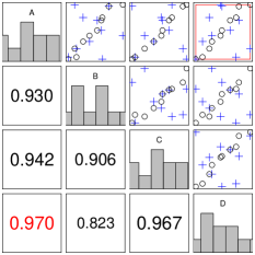
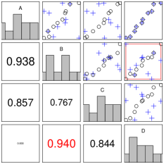
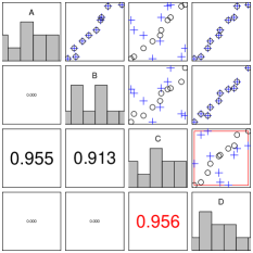
(a)	(b)	(c)
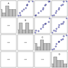
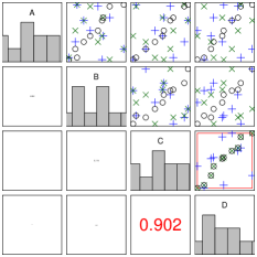
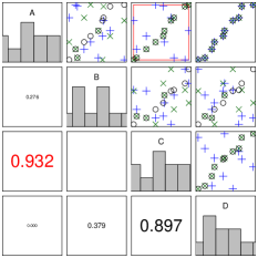
(d)	(e)	(f)

Figure 1. Example of visual data exploration with a toy data of 10 items. See the text for discussion.

Example of iterative data mining Consider the process in Fig. 1 showcasing a simple example of exploring a 4-dimensional data set of 10 items with attributes given by $A$, $B$, $C$, and $D$, respectively. The data set—shown with black hollow circles—exhibits a simple linear correlation structure in all dimensions. Initially, however, the user is unaware of the correlation structure and in his or her background model the attributes are uncorrelated. A sample of the initial background model obtained by permuting all columns independently at random, is shown with blue plus-signs in Fig. 1a. The goal of the system is to present the user with a maximally informative view of the data given the user’s current knowledge, i.e., the view in which the data and the background distribution differ the most. In this example, the possible views are given by 6 scatterplots over pairs of attributes ($AB$, $AC$, etc.).

In our example $AD$ is the most informative view. As the measure of informativeness in this example, we used the difference of the linear correlation between the actual data and the background distribution: if the user thinks two attributes are unrelated and observes that they are in fact correlated, it is both surprising and interesting to the user. The system presents the view $AD$, leading the user to update his or her internal model accordingly as shown in Fig. 1b, where columns $A$ and $D$ have been permuted together with the same permutation. Now, $BD$ is the most informative view. This is again absorbed by user, leading to Fig. 1c where columns $A$, $B$, and $D$ are permuted together with the same permutation. After the user has absorbed the information in view $CD$, he or she has assimilated all relations in the data after three views and the data and the background model match perfectly, as shown in Fig. 1d. Note that permuting the data (in contrast to other methods of modelling the data) preserves the marginal distributions in the columns, as evidenced by the histograms on the diagonals in Fig. 1.

Human-guided data exploration A clear shortcoming in the above described iterative data mining process is the fact that it cannot be guided by the user, since the system always tries to show the user the view in which the background distribution differs the most from the actual data. In other words, the user can only give feedback in the form of known or observed patterns, but the user cannot direct the exploration process to answer specific questions and the results are unpredictable, because—by definition!—the user is a priori unaware of which parts of the data that differ the most from his or her assumptions.

The fundamental question is then: how can the user focus the search on a specific hypothesis of his or her choice? Our insight is, instead of comparing the background distribution and the observed data, to compare two different hypothesis distributions both formed using the same background distribution, find the views where the hypothesis distributions differ most, and show how the data behaves in these views. In this way the user can establish which of the hypothesis is broken and by which data patterns (which the user can then add to the background knowledge). For example, the user might want to study whether two groups of attributes are independent. To this purpose the system would find views that most prominently show the differences between the two hypotheses, taking the already observed patterns into account (i.e., the user would not need to see the same information twice).

Consider again the toy example in Fig. 1. Let us assume that the user is interested only in the nature of the relation between attributes $C$ and $D$. A natural choice is to take the current background distribution and formulate two new distributions: one in which the relation between $C$ and $D$ is fully broken and one in which it is maintained, and then to find out which views are most informative concerning this relation.

If the user has not yet observed the data, the user’s background model is as shown in Fig. 1a. We can form Hypothesis 2 in which the relation between $C$ and $D$ is broken; in this case this implies the initial background model. In Hypothesis 1 attributes $C$ and $D$ are permuted together and their relation is preserved. Samples from these two hypotheses are shown in Fig. 1e, Hypothesis 2 with blue plus-signs and Hypothesis 1 with green crosses. Not surprisingly, the hypotheses differ most in the view $CD$ which the system then shows the user. Looking at the view $CD$ the user absorbs the fact that Hypothesis 2 is visually quite different from the data and hence he or she absorbs the relation of $C$ and $D$.

Assume now that the user has observed the view $AD$ and the background model is thus as shown in Fig. 1b. Hypothesis 2 corresponds to a model where attributes $A$ and $D$ are permuted together and $B$ and $C$ independently, and hypothesis 1 to a model where $A$, $C$, and $D$ are permuted together (if $A$ and $D$ are permuted together, and $C$ and $D$ are permuted together, then $A$, $C$, and $D$ must all be permuted together) and $B$ independently. Fig. 1f shows these two hypotheses. Now, the view $AC$ gives slightly more information than $CD$ about the relation of attributes $C$ and $D$! The explanation for this counterintuitive behaviour is that because the user knows that $A$ and $D$ are correlated, then the observation of correlation between $A$ and $C$ would reveal that $C$ and $D$ must be correlated. Therefore the system could choose to show the user the view $AC$ as well.

As this simple example shows, the constrained randomisation framework can be used to guide data exploration. In the simplest case (Fig. 1e) this guidance leads to predictable results (to learn about correlation between two attributes it is useful to look at the scatterplot of these attributes). However, if we take the user’s background knowledge into account we already obtain non-trivial insights, as shown by the informativeness of the view $AC$ in Fig. 1f. The situation becomes even more non-trivial when the background model is more complex (here the constraint is applied to whole views, but in practice the user might not absorb the view as a whole but only parts of it, e.g., cluster structures or outliers), instead of looking at relations of single variables we look at relations between groups of variables (a single view cannot show all relations between groups of many variables), and when the user is focusing only on a subset of data items. As an added bonus, we show later that the above described earlier iterative process in Figs. 1a–d is in fact a special case of our general framework.

Our framework has three important properties. (i) It is possible to incorporate existing and new information into the user’s background model, guiding the exploration, i.e., we maintain the property that the system tries to provide the user with maximally informative views of the data. (ii) It is possible to focus on exploring aspects in a subset of the data items and attributes. (iii) The framework allows the user to compare hypotheses concerning the data, so that specific questions can be answered. Notice that while we concentrate on two-dimensional scatterplots as the views to the data in this paper, the framework is totally general. The data types and the views can be anything.

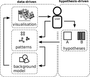
Figure 2. Human-Guided Data Exploration.

The basic high-level workflow in the EDA framework is shown in Fig. 2. The above described iterative exploration paradigm (explore) is described on the left side in the figure and is termed data-driven exploration. By augmenting the data-driven exploration by the hypothesis-driven exploration (shown on the right in the figure), we get the focus-oriented framework presented in this paper.

Related work This work is motivated by (puolamaki:2016, ) in which a similar system was constructed using constrained randomisation but without user guidance, see (DLS:16, ; kang2016, ; puolamaki2017, ) for approaches using the Maximum Entropy distribution. The Maximum Entropy method has been proposed (debie:2011a, ; debie2013, ) for modelling the user’s knowledge by a background distribution and it has been studied in the context of dimensionality reduction and EDA (DLS:16, ; kang2016, ; puolamaki2017, ). To the best of our knowledge, the framework presented in this paper is the first instance in which this background distribution can be updated both with direct interaction and user guidance, thus providing a principled method of EDA.

Many other special-purpose methods have been developed for active learning in diverse settings, e.g., in classification and ranking, as well as explicit models for user preferences. As these approaches are not targeted at data exploration, we do not review them here. Several special-purpose methods have been developed for visual iterative data exploration in specific contexts, e.g., for item-set mining and subgroup discovery (boley2013, ; dzyuba2013, ; vanleeuwen2015, ; paurat2014, ), information retrieval (ruotsalo2015, ), and network analysis (chau2011, ), also see (vismasterbook, ) for a summary.

Finally, the system presented here can also be considered an instance of visually controllable data mining (puolamaki2010, ), where the objective is to implement advanced data analysis methods understandable and efficiently controllable by the user. Our approach satisfies the properties of a visually controllable data mining method (puolamaki2010, , Sec. II B): (VC1) the data and the model space are presented visually, (VC2) there are intuitive visual interactions allowing the user to modify the model space, and (VC3) the method is fast enough for visual interaction.

Contributions We make the following contributions. (i) We present a novel framework for focused interactive iterative exploratory data analysis. The framework extends previous research by generalising the paradigm of iterative data mining to be user-focusable in terms of specific hypotheses specified by the user. (ii) We present an implementation of a free open source software tool (MIT license) realising the framework presented in this paper. Using the tool it is possible to interactively explore data, and all experiments in this paper are carried out using this tool. (iii) We demonstrate the three use-cases of exploring, focusing and comparing (with an emphasis on the latter two) using different datasets.

Outline In Sec. 2, we introduce the methods, and in Sec. 3, we present our novel framework for exploratory data analysis. In Sec. 4, we present our experimental evaluation together with an overview of our tool. We present both investigations carried out on real datasets and an evaluation of the scalability of our framework for EDA. We conclude with a discussion in Sec. 5.

2. Methods

We introduce the theory and methods related to the constrained randomisation of data matrices using tiles in this section.

Let $X$ be an $n\times m$ data matrix (data set) sampled from a distribution $P$. Here $X(i,j)$ denotes the $i$th element in column $j$. Each column $X(\cdot,j),\ j\in[m]$, is an attribute in the dataset, where we used the shorthand $[m]=\{1,\ldots,m\}$. Let $D$ be a finite set of domains (e.g., quantitative or categorical) and let $D(j)$ denote the domain of $X(\cdot,j)$. Also let $X(i,j)\in D(j)\textrm{ for all }i\in[n],\ j\in[m]$, i.e., all elements in a column belong to the same domain, but different columns can have different domains.

We define a permutation $\widehat{X}$ of the data matrix $X$ as follows.

Definition 2.1 (Permutation).

Let ${\mathcal{P}}$ denote the set of permutation functions of length $n$ such that $\pi:[n]\mapsto[n]$ is a bijection for all $\pi\in{\mathcal{P}}$, and denote by $\left(\pi_{1},\ldots,\pi_{m}\right)\in{\mathcal{P}}^{m}$ the vector of column-specific permutations. A permutation of the data matrix $X$ is then given as $\widehat{X}(i,j)=X(\pi_{j}(i),j)$.

We express the relations in the data matrix $X$ by tiles.

Definition 2.2 (Tile).

A tile is a tuple $t=(R,C)$, where $R\subseteq[n]$ and $C\subseteq[m]$.

The tiles considered here are combinatorial (in contrast to geometric), meaning that rows and columns in the tile do not need to be consecutive. In our illustrations in this paper we, however, use geometric tiles for clarity of presentation. In an unconstrained case, there are $(n!)^{m}$ allowed vectors of permutations. The tiles constrain the set of allowed permutations as follows.

Definition 2.3 (Tile constraint).

Given a tile $t=(R,C)$, the vector of permutations $\left(\pi_{1},\ldots,\pi_{m}\right)\in{\mathcal{P}}^{m}$ is allowed by $t$ iff the following condition is true for all $i\in[n]$, $j\in[m]$, and $j^{\prime}\in[m]$:

(1) $$i\in R\wedge j\in C\wedge j^{\prime}\in C\implies\pi_{j}(i)\in R\wedge\pi_{j}(i)=\pi_{j^{\prime}}(i).$$

Given a set of tiles $T$, a set of permutations is allowed iff it is allowed by all $t\in T$.

A tile defines a subset of rows and columns, and the rows in this subset are permuted by the same permutation function in each column in the tile. In other words, the relations between the columns inside the tile are preserved. Notice that the identity permutation is always an allowed permutation.

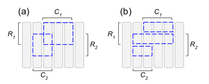
Figure 3. (a) A set of tiles, and (b) an equivalent tiling.

Our main problem is to draw samples from the uniform distribution over allowed permutations, defined as follows.

Definition 2.4 (Sampling problem).

Given a set of tiles $T$, the sampling problem is to draw samples uniformly at random from vectors of permutations in ${\mathcal{P}}^{m}$ such that the vectors of permutations are allowed by $T$.

The sampling problem is trivial when the tiles are non-overlapping. However, in the case of overlapping tiles, multiple constraints can affect the permutation of the same subset of rows and columns and this issue must be resolved. To this end, we need to define the equivalence of two sets of tiles.

Definition 2.5 (Equivalence of sets of tiles).

Let $T$ and $T^{\prime}$ be two sets of tiles. Let $P\subseteq\mathcal{P}^{m}$ be the vector of permutations allowed by $T$ and $P^{\prime}\subseteq\mathcal{P}^{m}$ be the vector of permutations allowed by $T^{\prime}$, respectively. We say that $T$ is equivalent to $T^{\prime}$ iff $P=P^{\prime}$.

Equivalence of sets of tiles hence means that the same constraints are enforced on the permutations.

We say that a set of tiles $\mathcal{T}$ such that no tiles overlap, is a tiling (we denote tilings using calligraphic letters). Next, we show that there always exists a tiling equivalent to a set of tiles.

Theorem 2.6 (Merging of tiles).

Given a set of (possibly overlapping) tiles $T$, there exists a tiling $\mathcal{T}$ that is equivalent to $T$.

Proof.

Let $t_{1}=(R_{1},C_{1})$ and $t_{2}=(R_{2},C_{2})$ be two overlapping tiles, as in Fig. 3(a). Each tile describes a set of constraints on the allowed permutations of the rows in their respective column sets $C_{1}$ and $C_{2}$. A tiling $\{t^{\prime}_{1},t^{\prime}_{2},t^{\prime}_{3}\}$ equivalent to $\{t_{1},t_{2}\}$ is given by:

$$t^{\prime}_{1}=(R_{1}\setminus R_{2},C_{1}),\qquad t^{\prime}_{2}=(R_{1}\cap R_{2},C_{1}\cup C_{2}),\qquad t^{\prime}_{3}=(R_{2}\setminus R_{1},C_{2}),$$

as shown in Fig. 3(b). Tiles $t^{\prime}_{1}$ and $t^{\prime}_{3}$ represent the non-overlapping parts of $t_{1}$ and $t_{2}$ and the permutation constraints by these parts can be directly met. Tile $t^{\prime}_{2}$ takes into account the combined effect of $t_{1}$ and $t_{2}$ on their intersecting row set, in which case the same permutation constraints must apply to the union of their column sets. It follows that these three tiles are non-overlapping and enforce the combined constraints of tiles $t_{1}$ and $t_{2}$. Hence, a tiling can be constructed by iteratively resolving overlap in a set of tiles until no tiles overlap. ∎

Notice that merging overlapping tiles leads to tiles with larger column sets (wider tiles) but smaller row sets (lower tiles). The limiting case is a fully-constrained situation where each row is a separate tile and only the identify permutation is allowed.

2.1. Algorithm for merging tiles

Merging a new tile into a tiling where, by definition, all tiles are non-overlapping, can be done efficiently using the Alg. 1, since we only need to consider the overlap between the new tile and the existing tiles in the tiling. This is similar to merging statements in (kalofolias:2016, ). Our algorithm has two steps and works as follows.

We first initialise a hash map (line 1). We then iterate over each row in $R$ for tile $t=(R,C)$ (lines 2–11). Each such row represents the IDs of the tiles with which the new tile overlaps at that row. For each row we check if this row has been seen before, i.e., if the row is a key in $S$ (line 4). If this is the first time this row is seen, we initialise $S(K)$ to be a tuple (line 5). We refer to the elements in the tuple by name as $S(K)_{\mathrm{rows}}$, and on line 6 we store the current row index in the tuple. On line 7 we store the unique tile IDs in the tuple $S(K)_{\mathrm{id}}$. If the row has been seen before, we update the row set associated with these tile IDs (line 9). After this step, $S$ contains tuples of the form (rows, id): id specifies the IDs of the tiles with which $t$ overlaps at the rows specified by rows.

We then proceed to update the tiling (lines 12–16). We first determine the currently largest tile ID in use (line 12), after which we iterate over the tuples in $S$. For each of the tuples we must update the tiles having IDs of $S(K)_{\mathrm{id}}$, and we therefore find the columns associated with these tiles on line 14. After this, we update the ID of the affected overlapping tiles on line 15, and increment the tile ID counter. Finally, we return the updated tiling on line 17. The time complexity of this algorithm is $\mathcal{O}{(nm)}$.

1

input : (1) A tiling $\mathcal{T}$ ($n\times m$ data matrix where each element is the ID of the tile it belongs to)

(2) A new tile $t=(R,C)$.

output : The tiling $\mathcal{T}$, where $t$ has been merged with $\mathcal{T}$.

2

3$S\leftarrow\texttt{HashMap}$;

4

5for $i\in R$ do

6       $K\leftarrow\mathcal{T}(i,C)$;

7       if  $K\notin\texttt{keys}(S)$ then

8             $S(K)\leftarrow\texttt{Tuple}$;

9             $S(K)_{\mathrm{rows}}\leftarrow\{i\}$;

10             $S(K)_{\textrm{id}}\leftarrow\texttt{unique}(\mathcal{T}(i,C))$;

11            

12       else

13             $S(K)_{\textrm{rows}}\leftarrow S(K)_{\textrm{rows}}\cup\{i\}$;

14            

15       end if

16      

17 end for

18

19$p_{\mathrm{max}}\leftarrow\max(\mathcal{T}(R,C))$;

20 for $K\in\texttt{keys}(S)$ do

21       $C^{\prime}=\left\{c\mid\mathcal{T}(S(K)_{\mathrm{rows}},c)\in S(K)_{\textrm{id}}\right\}$ ;

22       $\mathcal{T}\left(S(K)_{\textrm{rows}},C^{\prime}\right)\leftarrow p_{\mathrm{max}}+1$;   $p_{\mathrm{max}}\leftarrow p_{\mathrm{max}}+1$;

23      

24 end for

25return $\mathcal{T}$

Algorithm 1 Merging tiles. The function HashMap denotes a hash map. The value in a hash map $H$ associated with a key $x$ is $H(x)$ and $\texttt{keys}(H)$ gives the keys of $H$. The function Tuple creates a (named) tuple. An element $a$ in a tuple $w=(\mathrm{a},\mathrm{b})$ is accessed as $w_{\mathrm{a}}$. The function unique returns the unique elements of an array.

3. Exploration Framework

The task of the user in the exploratory framework shown in Fig. 2 is to compare two data samples, corresponding to different hypotheses, and draw conclusions based on this. In this section we present how the background model and these hypotheses are formed and their relation to typical exploratory data mining tasks.

Background model. The user’s knowledge concerning relations in the data are described by tiles (Def. 2.3). As the user views the data the user can highlight relations he or she has absorbed by tiles. For example, the user can mark an observed cluster structure with a tile involving the data points in the cluster and the relevant dimensions. We denote the set of user-defined tiles by ${\mathcal{T}}_{u}$. A sample from the background model is defined by first sampling a permutation vector uniformly from the set of permutation vectors allowed by the tiling ${\mathcal{T}}_{u}$ (Def. 2.4) and then obtaining the permuted data set (Def. 2.1).

Hypothesis. The hypothesis tilings specify the hypotheses that the user is investigating and provide a flexible method for investigating different questions concerning relations in the data.

Definition 3.1 (Hypothesis tilings).

Given a subset of rows $R\subseteq[n]$, a subset of columns $C\subseteq[m]$, and a $k$-partition of the columns given by $C_{1},\ldots,C_{k}$, such that $C=\cup_{i=1}^{k}{C_{k}}$ and $C_{i}\cap C_{j}=\emptyset$ if $i\neq j$, a hypothesis tiling is given by $\mathcal{T}_{H_{1}}=\{(R,C)\}$ and $\mathcal{T}_{H_{2}}=\cup_{i=1}^{k}{\{(R,C_{i})\}}$, respectively.

Because a hypothesis tiling defines a question about the data it can be specified before observing any data points.

The hypothesis tiling defines the items and attributes of interest and the relations between the attributes that the user is interested in. In our general framework, the user compares samples from two distributions, each sample corresponding to a hypothesis. These two samples are obtained by sampling permutations consistent with $\mathcal{T}_{1}=\mathcal{T}_{u}+\mathcal{T}_{H_{1}}$ and $\mathcal{T}_{2}=\mathcal{T}_{u}+\mathcal{T}_{H_{2}}$, respectively. We here use ’$+$’ with a slight abuse of notation to denote the operation of merging tilings into an equivalent tiling (Alg. 1). Hypothesis 1 ($\mathcal{T}_{1}$) corresponds to a hypothesis where all relations in $(R,C)$ are preserved, and hypothesis 2 ($\mathcal{T}_{2}$) to a hypothesis where there are no unknown (in addition to those relations in the background model) relations between attributes in the partitions $C_{1},\ldots,C_{k}$ of $C$. Views that show differences between these two hypotheses are most informative in describing how the data set differs with respect to these two hypotheses.

For example, if the columns are partitioned into two groups $C_{1}$ and $C_{2}$ the user is interested in relations between attributes in $C_{1}$ and $C_{2}$, but not in relations within $C_{1}$ or $C_{2}$. On the other hand, if the partition is full, i.e., $k=|C|$ and $|C_{i}|=1$ for all $i\in[k]$, then the user is interested in all relations between the attributes. In the latter case, the special case of $R=[n]$ and $C=[m]$ indeed reduces to the unguided iterative data mining in Figs. 1a–d. We define the following special cases of hypotheses.

Exploration is the data-driven scenario on the left in Fig. 2, where the user explores the data in order to discover interesting relations, without directing the search in any way. This is accomplished by comparing the original data with a sample corresponding to the user tiling. This is realised using the following hypothesis tilings: $\mathcal{T}_{H_{1}}=\{([n],[m])\}$ and $\mathcal{T}_{H_{2}}=\{([n],\{j\})\mid j\in[m]\}$. See Fig. 1a–d for an example.

Focusing means that the user wants to explore features in the data limited to a subset of items and attributes. As described in the introduction, it is often beneficial to focus on the interesting aspects in the data instead of removing the data outside one’s focus. Hence, this is a convenient way to focus on exploring a subset of the data. This is realised using the following hypothesis tilings: $\mathcal{T}_{H_{1}}=\{(R,C\}$ and $\mathcal{T}_{H_{2}}=\{(R,\{j\})\mid j\in C\}$, where $R$ and $C$ are the sets of rows and columns, respectively, of interest. See Fig. 1e–f for an example.

Most informative view. The only remaining problem to solve is how to find a view in which the distributions defined by the two hypotheses $\mathcal{T}_{1}$ and $\mathcal{T}_{2}$ differ the most. The answer to this question depends on the type of data and the visualisation chosen. For example, the visualisations or measures of difference would be different for categorical or real valued data. For real valued data we can use projections that mix attributes (such as principal components). In this work we consider only views that involve two attributes and can be shown as scatterplots over these attributes. The problem then reduces to finding the most informative of these views specified by a pair of attributes.

Here we use the following measure of interestingness to choose the maximally informative view presented to the user.

Definition 3.2 (Maximally informative view).

Given two data samples $X_{1}$ and $X_{2}$, the maximally informative view is given by columns $i$ and $j$ subject to

$$\operatorname*{arg\,max}_{i,j\in[m],\;i\neq j}|\mathrm{cor}(X_{1}(\cdot,i),X_{1}(\cdot,j))^{2}-\mathrm{cor}(X_{2}(\cdot,i),X_{2}(\cdot,j))^{2}|,$$

where $\mathrm{cor}$ denotes Pearson’s correlation.

While we have here chosen to use correlation due to ease of interpretability for the user when considering two-dimensional data projections, it should be noted that also other measures of distance between distributions can be used.

4. Experiments

In this section we first describe a software tool showcasing our method. We then continue with a discussion of the scalability of the method presented in this paper. Finally, we consider use of the tool in the exploration of real-world datasets.

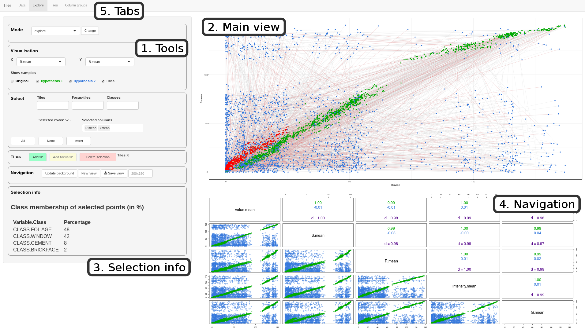
Figure 4. The main user interface of the software tool.

$n$	$m$	$k$	$t_{\mathrm{init}}$ ($s$)	$t_{\mathrm{permute}}$ ($s$)	$t_{\mathrm{max,add}}$ ($s$)
$5000$	$50$	$25$	$0.04$	$0.01$	$0.06$
$5000$	$50$	$50$	$0.04$	$0.02$	$0.07$
$5000$	$50$	$100$	$0.03$	$0.02$	$0.08$
$5000$	$100$	$25$	$0.08$	$0.03$	$0.09$
$5000$	$100$	$50$	$0.08$	$0.04$	$0.18$
$5000$	$100$	$100$	$0.07$	$0.03$	$0.12$
$10000$	$50$	$25$	$0.07$	$0.04$	$0.14$
$10000$	$50$	$50$	$0.08$	$0.06$	$0.20$
$10000$	$50$	$100$	$0.07$	$0.06$	$0.41$
$10000$	$100$	$25$	$0.34$	$0.10$	$0.21$
$10000$	$100$	$50$	$0.15$	$0.14$	$0.34$
$10000$	$100$	$100$	$0.15$	$0.07$	$0.53$

Table 1. Scalability of the algorithm. The columns show the number of rows ($n$) and columns ($m$) in the tiling and the number of user tiles ($k$). The other columns show the time in seconds to initialise the tiling, permute the data matrix, and the maximum time for adding a tile.

4.1. Software tool

We developed an interactive tool to demonstrate the use of the above presented randomisation approach for exploratory data analysis of generic data sets containing real-valued and categorical attributes. The tool runs in a web browser and is developed in R (Rproject, ) using shiny (shiny, ). The tool is released as free software under the MIT license. Fig. 4 shows the main user interface of the software tool.

The tool supports the full framework described in Sec. 3, including the special cases exploration (the original iterative data mining framework) and focusing. The tool is interactive and selection of data items can be made by brushing. Different hypotheses can be formed by grouping columns. Tiles can both be added and removed and different data projections can be chosen by the user. The tool models the two hypotheses being compared by the user and shows the data points belonging to samples from these models in different colours (Hypothesis 1 in green and Hypothesis 2 in blue). The tool also suggests the maximally informative view (Def. 3.2). For simplicity we here chose to use scatterplots of attribute pairs, but it would be straightforward to supplement it with visualisations using, e.g., projections as in (puolamaki:2016, ; puolamaki2017, ). To help the user understand the data better, class information of selected points (for data having classes) is shown. Finally, a scatterplot matrix shows a few of the most interesting variables in the data, which helps the user to quickly get an overview of the data and to discover patterns

4.2. Scalability

We here investigate the performance of the tiling algorithm in terms of wall-clock running time for interactive use. The experiments were run on a MacBook Pro laptop with a 2.5 GHz Intel Core i7 processor and R 3.4.3 (Rproject, ).

The results are presented in Tab. 1. We initialise a tiling to have $n\in\{5000,10000\}$ rows and $m\in\{50,100\}$ columns (this gives $t_{\mathrm{init}}$). We then add $k\in\{25,50,100\}$ randomly created tiles (the dimensions of the tile are 10% of the row and column space of the data matrix, respectively) to the tiling and permute the data, giving $t_{\mathrm{permute}}$. The maximum time needed to add a tile to a tiling (essentially running Alg. 1) is given by $t_{\mathrm{max,add}}$.

We note that the initialisation time and time needed to permute the data is negligible. The time needed to add a tile increases with the size of the data. The method is clearly fast enough for interactive use, since even for a dataset with a million elements addition of a new tile and permutation of the data can be done in less than a second. It should also be noted that large datasets can typically be downsampled, if needed, without loss of characteristics for visual exploration, because usually it is not possible to visualise millions of data points anyway.

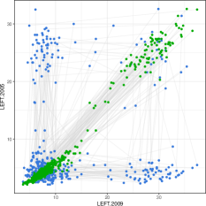
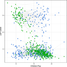
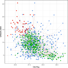
(a)	(b)	(c)

Figure 5. German Socio-Economic Data. (a) Task 1, the first and (b) the tenth view. (c) Task 2, the third view.

4.3. German Socio-Economic Data

The German socio-economic dataset (boley2013, ; kang:2016a, ) consists of records from 412 administrative districts in Germany. Each district is represented by 46 attributes including socio-economic and political attributes in addition to attributes such as type of the district (rural/urban), area name/code, state, region and the geographic coordinates of each district center. The socio-ecologic attributes include, e.g., population density, age and education structure, economic indicators (e.g., GDP growth, unemployment, income), and structure of the labour market in terms of workforce in different sectors. The political attributes include election results of the five major political parties (CDU/CSU,e SPD, FDP, Green, and Left) for the German federal elections of 2005 and 2009, respectively, as well as the election participation.

Task 1: Exploration As we start without any prior knowledge our first task is to explore the data using our tool to gain insight into the main features in the data. The first view provided by the tool is shown in Fig. 5a. The green points correspond to Hypothesis 1 maintaining all correlations between attributes, while blue points correspond to Hypothesis 2 breaking the correlations. The locations of the actual data points, not shown in this view, match the sample from Hypothesis 1. The view reveals, not surprisingly, that there is a strong positive association between the election results for the Left party in 2005 and 2009. We also see that the points in the sample from Hypothesis 1 (and thus in the data as well) are clustered into two groups (corresponding to different areas). We note these observations by adding two constraints in the form of tiles that (i) connect attributes Left 2005 and Left 2009 , and (ii) connect the points in one of the observed clusters. After updating the background distributions, the samples from both hypotheses look similar, i.e., our constraints capture the structure of the data wrt. the attributes in this view. Next, we request a new view.

The next view shows a strong negative association between service and production workforce. We add a tile constraint for all data points and the attributes in this view and update the background distribution. Subsequent iterations reveal further dependencies (association between votes for the Green party (resp. SDP, CDU, FDP, and the election participation) in 2005 and 2009, unemployment and youth unemployment, as well as, manufacturing and production workforce). All these views increase our understanding of the data, although they are not very surprising.

The tenth view reveals something more interesting (Fig.  5b). We notice that the data points separate into two groups, mainly on the attribute Left 2009 , though the group with higher values of Left 2009 has lower values for Children population . We add a tile constraint for the set of districts in the upper left corner, and update the background distribution. The next view of Left 2009 and Unemployment shows a similar separation. We use our tool to show the points in the tile added in the previous view and observe, that the same sets of points are clustered also in this view. Furthermore, the clustered sets of districts coincide almost perfectly with the sets of clustered districts from the first view. We further investigate this by changing the projection in the main view to geographical coordinates, noticing that the districts in the former East Germany together with a couple of districts in Saarland separate in terms of more votes for the Left. Upon further analysis, it becomes apparent that the most visible effect in the data is the division into East and West Germany, reflected mostly in the popularity of the Left party, but visible in, e.g., the age structure and economic indicators, too.

Task 2: Focusing on weaker signals When exploring the data, we observed several characteristics separating the former East and West Germany. Now, we want to focus on relations between other attributes, i.e., we want to discover relations that do not reflect the historical division between East and West Germany.

We choose the Focus-mode in our tool and define a focus tile covering all districts and the following attributes: CDU 2009 , FDP 2009 , Green 2009 , SDP 2009 , Election participation 2009 , Population density , all age structure-related attributes, Income , GDP growth 2009 , Unemployment , and the geographical coordinates (16 attributes in total). Thus, we focus on the 2009 election results while leaving the correlated 2005 elections result attributes outside the focus. Furthermore, we leave Left 2009 outside the focus area, due to its now known strong effect.

After defining the focus area into the tool, we obtain a view where we observe a negative association between Unemployment and Children population . We add a tile constraining this observation and proceed. The next view shows a negative association between Unemployment and Election participation 2009 and after adding a tile constraining this we proceed. The third view (Fig. 5c) shows Old population and Green 2009 . Here we see that there are roughly two kinds of outliers. In the lower right corner districts have a larger old population and vote less for the Green party. These correspond mainly to districts in Eastern Germany. The other set of outliers are the districts with few old people and voting more for the Green (the red selection in Fig. 5c). We add a tile constraint for both of these outlier sets and the set of remaining districts (i.e., we partition the districts in three sets and add a tile constraint for each set separately). When proceeding further we are shown Middle-aged population and Green 2009 . Here we see again outliers with a high support for the Green party. We observe that these outliers coincide almost perfectly with the outliers with high support of the Green party from the previous step. There is hence a set of districts characterised by a high support of the Green party, and a large middle-aged and small old population. Upon further inspection, we observe that these are mainly urban districts including the largest cities in Germany.

In addition to discovering the distinction between East and West Germany, we identified a subset of urban districts that are outliers in terms of their support for the Green party and, e.g., the age distribution of the population. The associations we discovered in a straight-forward manner using visual EDA, are among the ones found in (boley2013, ) with a method using pattern mining techniques.

4.4. UCI Image Segmentation data

As a second use case, we consider the Image Segmentation dataset from the UCI machine learning repository (Lichman:2013, ) with 2310 samples, 19 real-valued attributes and one class attribute.

Task 3: Focusing During Exploration We know apriori that the dataset contains several correlated attributes. We, however, start by exploring the data and observe from the first view (and the scatterplot matrix of the tool) that there is a set of 330 points (belonging to the class sky ) in the upper-right corner clearly separated in terms of value , B , G , R , and Intensity (Fig. 6a). We add a tile constraining all these attributes and proceed. The next view shows us that, in fact, the same set of points also cluster in terms of value and excess-R . We add another tile constraining this.

Having defined two tile constraints for the set of points from the class sky , we want to focus our exploration on other points, while keeping the already defined tiles. Thus, we define a hypothesis tiling as follows. We select the 1980 points outside the class sky as our focus rows $R$. For the attributes, we choose a grouping $C=C_{1}\cup C_{2}\cup C_{3}$ in which the attributes related to RGB-values are grouped into a single group $C_{1}=\{\texttt{\scalebox{0.7}[1.0]{value}},\texttt{\scalebox{0.7}[1.0]{B}},\texttt{\scalebox{0.7}[1.0]{G}},\texttt{\scalebox{0.7}[1.0]{R}},\texttt{\scalebox{0.7}[1.0]{Intensity}},\texttt{\scalebox{0.7}[1.0]{excess-B}},$ $\texttt{\scalebox{0.7}[1.0]{excess-G}},\texttt{\scalebox{0.7}[1.0]{excess-R}}\}$, and $C_{2}=\{\texttt{\scalebox{0.7}[1.0]{saturation}}\}$ and $C_{3}=\{\texttt{\scalebox{0.7}[1.0]{hue}}\}$ form individual groups. After updating our hypotheses, we are shown the view with attributes hue and excess-G (Fig. 6b). In this view, the set of points in the upper right (belonging to the class grass ) form a clear cluster, and 48 points from the classes window and foliage are outliers with hue at 0 in the middle. We add tile constraints for these sets of points, update the background distributions and request a new view. The next view then (Fig. 6c) shows further structure in terms of saturation and R .

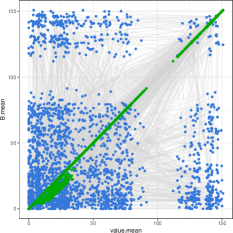
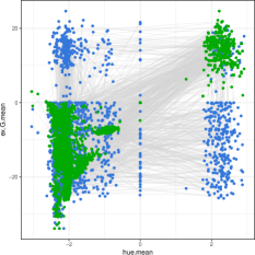
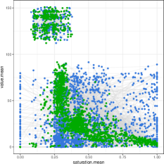
(a)	(b)	(c)

Figure 6. Segmentation data. (a) Exploration-mode, the first view. (b) Comparison-mode, the first and (c) the second view.

5. Conclusions

In this paper we presented the Human-Guided Data Exploration (HGDE) framework, generalising and extending previous research in the field of iterative data mining.

The user can direct the exploration process to relations of interest, so that specific questions (posed as hypotheses in the framework) can be answered. This places the iterative data mining process on an informed basis, as the user is able to steer the process and can hence better anticipate where the process leads. This is in contrast to prior work where no control was possible and the data mining process was unpredictable. It should be noted that sometimes we do want to be surprised, though, and this uninformed exploration is indeed a special case of the general framework presented here.

The HGDE framework is based on constrained randomisation of the data, and the knowledge of the user is communicated by constraints on permutations of the data. We formalise these constraints, describing relations between the data items and the data attributes, as tiles (subsets of rows and columns). The tiles are conceptually simple and they are parametrised by a subset of rows and attributes of the data: a tile means that the user has absorbed the relations of the data points in the respective attributes. We demonstrated empirically that our method is feasible for interactive use also with large datasets.

Although the constrained permutation scheme is conceptually simple, it is also computationally efficient, which is an advantage over other modelling techniques in many cases. Also, permutation of the data using the scheme used here is a non-parametric method with very few distributional assumptions, keeping the column margins intact (since no new values are introduced, they are only re-ordered). This ensures that the user is not surprised due to spurious modelling errors, instead, any observed structure (or lack thereof) relates to the internal relationships between the attributes. A further advantage of the permutation scheme is that it is agnostic with regards to the domain of the data attributes, i.e., since the data items are shuffled within each column it does not matter what the domains of the columns are.

To showcase the interactive use of the method, we developed a free open-source tool to demonstrate these concepts, using which we also performed the empirical evaluation in this paper. Using real-world datasets, we demonstrated the utility of being able to focus the data exploration process, so that novel aspects of the data are revealed, taking into account those features of the data the user has already assimilated.

The HGDE framework presented in this paper, and realised in the form of the tool, has several potential applications in explorative data analysis tasks. Explorative data analysis is crucial for successful data analysis and mining. The framework presented here provides a simple and functional approach to allowing the user to direct his or her interest towards answering complex hypotheses concerning the data. While there are methods for the same objectives, ours is the first to present the task of exploration in a principled way such that: (i) the user’s background knowledge is modelled and the user is always shown informative views, (ii) the user can ask specific questions of the data using the same framework, and (iii) the problem is solvable using an efficient permutation sampling methodology, as demonstrated by the open source application published in conjunction with this paper.

The power of human-guided data exploration stems from the fact that typical data sets have a huge number of interesting patterns. However, the patterns that are interesting for a user depend on the task at hand. A non-interactive data mining method is therefore restricted to either show generic features of data (which may be obvious to an expert) or then output unusably many patterns (a typical problem, e.g., in frequent pattern mining: there are easily too many patterns for the user to absorb). Our framework is a solution to this problem: by integrating the human background knowledge and focus—formulated as a mathematically defined hypothesis—we can at the same time guide the search towards topics interesting to the user at any particular moment and take the user’s prior knowledge into account in an understandable and efficient way.

While we have demonstrated our approach on real-valued and categorical data sets and the views used are scatterplot over pairs of attributes, the approach is generic and can be used for different data types and different views of the data. An interesting future problem would be to generalise this work to other data types, such as time series, networks etc. It would also be interesting to study how these approaches could be used to explore the model spaces of machine learning algorithms such as classifiers (henelius2014, ).

Acknowledgements This work has been supported by the Academy of Finland (decisions 288814 and 313513).

References

- [1] M. Boley, M. Mampaey, B. Kang, P. Tokmakov, and S. Wrobel. One click mining—interactive local pattern discovery through implicit preference and performance learning. In KDD-IDEA, pages 27–35, 2013.
- [2] W. Chang, J. Cheng, J. Allaire, Y. Xie, and J. McPherson. shiny: Web Application Framework for R, 2017. R package version 1.0.5.
- [3] D. Chau, A. Kittur, J. Hong, and C. Faloutsos. Apolo: making sense of large network data by combining rich user interaction and machine learning. In CHI, pages 167–176, 2011.
- [4] T. De Bie. An information theoretic framework for data mining. In KDD, pages 564–572, 2011.
- [5] T. De Bie. Maximum entropy models and subjective interestingness: an application to tiles in binary databases. Data Min. Knowl. Discov., 23(3):407–446, 2011.
- [6] T. De Bie. Subjective interestingness in exploratory data mining. In IDA, pages 19–31, 2013.
- [7] T. De Bie, J. Lijffijt, R. Santos-Rodriguez, and B. Kang. Informative data projections: a framework and two examples. In ESANN, pages 635 – 640, 2016.
- [8] V. Dzyuba and M. van Leeuwen. Interactive discovery of interesting subgroup sets. In IDA, pages 150–161, 2013.
- [9] M. A. Fisherkeller, J. H. Friedman, and J. W. Tukey. Prim-9: An interactive multidimensional data display and analysis system. Technical report, Princeton University, 1974.
- [10] S. Hanhijärvi, M. Ojala, N. Vuokko, K. Puolamäki, N. Tatti, and H. Mannila. Tell me something i don’t know: randomization strategies for iterative data mining. In KDD, pages 379–388, 2009.
- [11] A. Henelius, K. Puolamäki, H. Boström, L. Asker, and P. Papapetrou. A peek into the black box: exploring classifiers by randomization. Data Mining and Knowledge Discovery, 28(5–6):1503–1529, 2014.
- [12] J. Kalofolias, E. Galbrun, and P. Miettinen. From sets of good redescriptions to good sets of redescriptions. In ICDM, pages 211–220, 2016.
- [13] B. Kang, J. Lijffijt, R. Santos-Rodríguez, and T. De Bie. Subjectively interesting component analysis: Data projections that contrast with prior expectations. In KDD, pages 1615–1624, 2016.
- [14] B. Kang, J. Lijffijt, R. Santos-Rodríguez, and T. De Bie. Subjectively interesting component analysis: Data projections that contrast with prior expectations. In KDD, pages 1615–1624, 2016.
- [15] B. Kang, K. Puolamäki, J. Lijffijt, and T. De Bie. A tool for subjective and interactive visual data exploration. In ECML-PKDD, pages 3–7, 2016.
- [16] D. Keim, J. Kohlhammer, G. Ellis, and F. Mansmann, editors. Mastering the Information Age: Solving Problems with Visual Analytics. EG Association, 2010.
- [17] M. Lichman. UCI machine learning repository, 2013.
- [18] J. Lijffijt, P. Papapetrou, and K. Puolamäki. A statistical significance testing approach to mining the most informative set of patterns. DMKD, 28(1):238–263, 2014.
- [19] D. Paurat, R. Garnett, and T. Gärtner. Interactive exploration of larger pattern collections: A case study on a cocktail dataset. In KDD-IDEA, pages 98–106, 2014.
- [20] K. Puolamäki, B. Kang, J. Lijffijt, and T. De Bie. Interactive visual data exploration with subjective feedback. In ECML-PKDD, pages 214–229, 2016.
- [21] K. Puolamäki, E. Oikarinen, B. Kang, J. Lijffijt, and T. D. Bie. Interactive visual data exploration with subjective feedback: An information-theoretic approach, 2017. arXiv:1710.08167 [stat.ML].
- [22] K. Puolamäki, P. Papapetrou, and J. Lijffijt. Visually controllable data mining methods. In ICDMW, pages 409–417, 2010.
- [23] R Core Team. R: A Language and Environment for Statistical Computing. R Foundation for Statistical Computing, Vienna, Austria, 2018.
- [24] T. Ruotsalo, G. Jacucci, P. Myllymäki, , and S. Kaski. Interactive intent modeling: Information discovery beyond search. CACM, 58(1):86–92, 2015.
- [25] J. W. Tukey. Exploratory data analysis. Addison-Wesley.
- [26] M. van Leeuwen and L. Cardinaels. Viper — visual pattern explorer. In ECML-PKDD, pages 333–336, 2015.