Seesaw Dirac neutrino mass through dimension-6 operators

Abstract

In this paper, a followup of CentellesChulia:2018gwr , we describe the many pathways to generate Dirac neutrino mass through dimension-6 operators. By using only the Standard Model Higgs doublet in the external legs one gets a unique operator $\frac{1}{\Lambda^{2}}\,\bar{L}\,\bar{\Phi}\,\bar{\Phi}\,\Phi\,\nu_{R}$. In contrast, the presence of new scalars implies new possible field contractions, which greatly increase the number of possibilities. Here we study in detail the simplest ones, involving $SU(2)_{L}$ singlets, doublets and triplets. The extra symmetries needed to ensure the Dirac nature of neutrinos can also be responsible for stabilizing dark matter.

I Introduction

Elucidating the nature of neutrinos constitutes a key open challenge in particle physics. The detection of neutrinoless double-beta decay - ${0\nu}\beta\beta$ - would establish the Majorana nature of at least one neutrino Schechter:1981bd So far, however, the experimental searches KamLAND-Zen:2016pfg ; GERDA:2018 ; MAJORANA:2008 ; CUORE:2018 ; EXO-2018 ; Arnold:2016bed for ${0\nu}\beta\beta$ have not borne a positive result, leaving us in the dark concerning whether neutrinos are their own anti-particles or not. One should stress that, although Dirac neutrinos are not generally expected within a gauge theoretic framework Schechter:1980gr , they arise in models with extra dimensions Chen:2015jta ; Addazi:2016xuh , where the $\nu_{R}$ states are required for the consistent high energy completion of the theory. Dirac neutrinos also emerge in conventional four dimentional gauge theories with an adequate extra symmetry. One appealing possibility is the quarticity symmetry, which was originally suggested in Chulia:2016ngi ; Chulia:2016giq ; CentellesChulia:2017koy . This mechanism uses a version of $U(1)_{L}$ lepton number symmetry broken into its subgroup $Z_{4}$.

In summary, there has been recently a growing interest in Dirac neutrinos Heeck:2013rpa ; Abbas:2013uqh ; Ma:2014qra ; Okada:2014vla ; Ma:2015rxx ; Ma:2015raa ; Ma:2015mjd ; Valle:2016kyz ; Bonilla:2016zef ; Bonilla:2016diq ; Chulia:2016ngi ; Chulia:2016giq ; Reig:2016ewy ; Ma:2016mwh ; Wang:2016lve ; Borah:2016zbd ; Abbas:2016qbl ; Yao:2017vtm ; Ma:2017kgb ; CentellesChulia:2017koy ; Borah:2017leo ; Wang:2017mcy ; Bonilla:2017ekt ; Hirsch:2017col ; Srivastava:2017sno ; Borah:2017dmk ; Yao:2018ekp ; Chen:2015jta ; Addazi:2016xuh ; CentellesChulia:2017sgj ; Fonseca:2018ehk ; Helo:2018bgb ; Reig:2018mdk . The many pathways to generate Dirac neutrino mass through generalized dimension-5 operators a la Weinberg have been described in Ref. CentellesChulia:2018gwr . It has been shown that the symmetry responsible for “Diracness” can always be used to stabilize a WIMP Dark Matter candidate, thus connecting the Dirac nature of neutrinos with the stability of Dark Matter.

In this letter we take the point of view that neutrinos are Dirac fermions, extending the results of CentellesChulia:2018gwr to include the analysis of seesaw operators that lead to Dirac neutrino mass at dimension 6 level. Using only the Standard Model Higgs doublet in the external legs one is lead to a unique operator $\frac{1}{\Lambda^{2}}\,\bar{L}\,\bar{\Phi}\,\bar{\Phi}\,\Phi\,\nu_{R}$. However the presence of new scalar bosons beyond the standard Higgs doublet implies many new possible field contractions. We also notice that, also here and quite generically, the extra symmetries needed to ensure the Dirac nature of neutrinos can also be made responsible for stability of dark matter.

The paper is organized as follows. In Section II we discuss the various dimension-6 operators that can give rise to Dirac neutrinos. For simplicity we restrict ourselves to the simplest cases of scalar singlets ($\chi$), doublets ($\Phi$) and triplets ($\Delta$) of $SU(2)_{L}$. We also discuss the Ultra-Violet (UV) complete theories associated to each operator. All these completions fall under one of the five distinct topologies, which we discuss, along with the associated generic neutrino mass estimate. In Section III we explicitly construct and discuss all the UV-complete dimension-6 models involving only Standard Model fields. In Section IV we discuss the various UV-completions of the dimension-6 operators involving only $SU(2)_{L}$ singlet $\chi$ and doublet $\Phi$ scalars. In Section V we consider the possible UV-completions of the dimension-6 seesaw operators involving all three types of Higgs scalars, singlet $\chi$, doublet $\Phi$ and triplet $\Delta$. In Section VI we discuss the UV-completion of the dimension-6 operator involving the doublet $\Phi$ and triplet $\Delta$ scalars. In Section VII we present a short summary and discussion.

II Operator Analysis

We begin our discussion by looking at the possible dimension-6 operators that can lead to naturally small Dirac neutrino masses. In order to cut down the number of such operators in this work we will limit our discussion only to operators involving scalar singlet ($\chi$), doublet ($\Phi$) and triplet ($\Delta$) representations of the weak gauge group $SU(2)_{L}$. The discussion can be easily extended to other higher $SU(2)_{L}$ multiplets. The general form of such dimension-6 operators is given by

$$\frac{1}{\Lambda^{2}}\,\bar{L}\otimes X\otimes Y\otimes Z\otimes\nu_{R}$$ (1)

where $L=(\nu_{L},e_{L})^{T}$ is the lepton doublet, $\nu_{R}$ are the right handed neutrinos which are singlet under Standard Model gauge group and $X,Y,Z$ denote scalar fields which are singlets under $SU(3)_{c}$, transforming under $SU(2)_{L}$ and carrying appropriate $U(1)_{Y}$ charges such that the operator is invariant under the full Standard Model gauge symmetry. Moreover, $\Lambda$ is the cutoff scale above which the full UV-complete theory must be taken into account. For sake of simplicity, throughout this work we will suppress all flavor indices of the fields. The $\mathrm{SU(3)_{C}\otimes SU(2)_{L}\otimes U(1)_{Y}}$ symmetry is broken by the vacuum expectation values (vev) of the scalars. After symmetry breaking the neutrinos acquire naturally small Dirac masses.

Invariance under $\mathrm{SU(3)_{C}\otimes SU(2)_{L}\otimes U(1)_{Y}}$ dictates that, if $X$ transforms as a $n$-plet under $SU(2)_{L}$, then $Y\otimes Z$ must transform either as a $n+1$-plet or a $n-1$-plet. This leaves many possible choices for the scalars $X,Y,Z$, as we now discuss.

For example, if we take $X$ to be a singlet $\chi$, then $Y\otimes Z$ should transform as a doublet of $SU(2)_{L}$. Restricting ourselves only to representations up to triplets of $SU(2)_{L}$ , one possibility is $Y\otimes Z\equiv\chi\otimes\bar{\Phi}$, where $\bar{\Phi}$ denotes a scalar doublet of $SU(2)_{L}$ but with hypercharge opposite to that of $\Phi$. It can be either $\Phi^{\dagger}$ or $\Phi^{c}$, depending on the particular $SU(2)_{L}$ contraction. The only other option is $Y\otimes Z\equiv\bar{\Phi}\otimes\Delta_{0}$ or $Y\otimes Z\equiv\Phi\otimes\Delta_{-2}$ where $\Delta_{i}$; $i=0,-2$ is a scalar triplet of $SU(2)_{L}$. Note that here, depending on the choice of $\Phi$ or $\bar{\Phi}$, there are two possible $U(1)_{Y}$ charge assignments for $\Delta_{i}$ i.e. $\Delta_{0}$ with $U(1)_{Y}=0$ and $\Delta_{-2}$ with $U(1)_{Y}=-2$.

Taking $X$ as a doublet $\bar{\Phi}$ or $\Phi$, then $Y\otimes Z$ must transform either as a singlet or a triplet under $SU(2)_{L}$ symmetry. Thus we could have $Y\otimes Z\equiv\chi\otimes\chi$ which is only allowed if $X=\bar{\Phi}$. The other option is to have $Y\otimes Z\equiv\chi\otimes\Delta_{i}$; $i=0,-2$. These operators are the same as already discussed for $X=\chi$ case . Apart from these, as far as transformation under $SU(2)_{L}$ is concerned, there are two new possibilities, namely $Y\otimes Z\equiv\Delta\otimes\Delta$ and $Y\otimes Z\equiv\bar{\Phi}\otimes\Phi$. The latter is the only dimension-6 operator which can be written down with only Standard Model scalar fields . For the operator $Y\otimes Z\equiv\Delta\otimes\Delta$ there are several possibilities depending on the hypercharge of $\Delta$, as listed in Table 1. If $X\sim 3$ under $SU(2)_{L}$ symmetry, it is easy to see that, restricting up to triplet representations of $SU(2)_{L}$, no new operator can be written. Each of these operators can lead to different possible $SU(2)_{L}$ contractions which in turn select the type of new fields needed in a UV-complete model . The resulting dimension-6 operators along with the number of possible UV-completions in each of the cases are summarized in Table 1.

$X$	$Y$	$Z$	Operator	Diagrams	$X$	$Y$	$Z$	Operator	Diagrams
$\mathbf{1}$	$\mathbf{1}$	$\mathbf{2}$	$\bar{L}\,\chi\,\chi\,\bar{\Phi}\,\nu_{R}$	$10$	$\mathbf{2}$	$\mathbf{2}$	$\mathbf{2}$	$\bar{L}\,\bar{\Phi}\,\bar{\Phi}\,\Phi\,\nu_{R}$	$15$
$\mathbf{1}$	$\mathbf{2}$	$\mathbf{3}$	$\bar{L}\,\chi\,\bar{\Phi}\,\Delta_{0}\,\nu_{R}$	$16$	$\mathbf{1}$	$\mathbf{1}$	$\mathbf{2}$	$\bar{L}\,\bar{\chi}\,\chi\,\bar{\Phi}\,\nu_{R}$	$15$
$\mathbf{1}$	$\mathbf{2}$	$\mathbf{3}$	$\bar{L}\,\chi\,\Phi\,\Delta_{-2}\,\nu_{R}$	$16$	$\mathbf{2}$	$\mathbf{3}$	$\mathbf{3}$	$\bar{L}\,\bar{\Phi}\,\bar{\Delta}_{0}\,\Delta_{0}\,\nu_{R}$	$31$
$\mathbf{2}$	$\mathbf{3}$	$\mathbf{3}$	$\bar{L}\,\bar{\Phi}\,\Delta_{0}\,\Delta_{0}\,\nu_{R}$	$16$	$\mathbf{2}$	$\mathbf{3}$	$\mathbf{3}$	$\bar{L}\,\bar{\Phi}\,\bar{\Delta}_{-2}\,\Delta_{-2}\,\nu_{R}$	$26$
$\mathbf{2}$	$\mathbf{3}$	$\mathbf{3}$	$\bar{L}\,\Phi\,\Delta_{0}\,\Delta_{-2}\,\nu_{R}$	$27$

Table 1: Possible $SU(2)_{L}$ assignments for the scalars $X$, $Y$, $Z$; the allowed operators and number of associated UV-complete models in each case. Here $\bar{\Phi}$ denotes either $\Phi^{\dagger}$ or $\Phi^{c}$, depending on the particular $SU(2)_{L}$ contractions. Note that the hypercharge of $\bar{\Phi}$ has the opposite sign than the hypercharge of $\Phi$. Similar notation is used for other scalar multiplets.

It is important to notice that the dimension-6 operators listed in Table 1 will give the leading contribution to neutrino mass only in scenarios where other lower dimensional operators are forbidden by some symmetry. Such scenarios can arise in context of many symmetries ranging from $U(1)_{X}$ symmetries Ma:2014qra ; Ma:2015mjd to abelian discrete $Z_{n}$ symmetries Chulia:2016ngi ; Bonilla:2016zef ; Bonilla:2016diq ; Reig:2016ewy ; Reig:2018mdk up to various types of more complex flavor symmetries containing non-abelian groups Chulia:2016giq ; CentellesChulia:2017koy ; Bonilla:2017ekt . Keeping this in mind, Table 1 is divided into two columns. The operators in the left column are those for which the lower dimensional operators can be forbidden by $U(1)_{X}$ or $Z_{n}$ symmetries. The operators in the right column will not be leading operators for neutrino mass in such case, but will require, for example, a soft breaking of such symmetries. Another appealing possibility is to have two copies of the scalars involved. Alternatively, one may use more involved symmetries involving non-abelian discrete flavor symmetries. We will further discuss this issue in latter sections.

Also, notice that the number of UV-complete models for similar type of operators e.g. $\bar{L}\,\chi\,\chi\,\bar{\Phi}\,\nu_{R}$ and $\bar{L}\,\bar{\chi}\,\chi\,\bar{\Phi}\,\nu_{R}$ are different. This is because, while counting the number of models, we have also taken into account the possible differences under the symmetry forbidding lower dimensional operators. Apart from Hermitian conjugated (h.c.) counterparts which are not listed, there are also other possibilities beyond the operators listed in Table 1, where one or more hypercharge neutral fields i.e. $\chi_{0}$ or $\Delta_{0}$, is replaced by the corresponding $\bar{\chi}$ or $\bar{\Delta}_{0}$. These possibilities are not listed here as they do not give rise to new operators, as far as only Standard Model symmetries are concerned. However, they can be potentially differentiated by other symmetries such as those forbidding the lower dimensional operators. We will also briefly discuss such possibilities in latter sections whenever they arise.

We find that all possible UV-completions of the operators listed in Table 1 can be arranged into five distinct topologies for the Feynman diagrams of neutrino mass generation. For lack of better names, we are calling these five topologies as $T_{i}$, $i\in\{1,2,3,4,5\}$. These topologies are shown in Fig. 1.

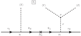
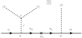
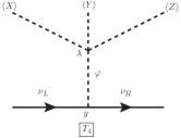
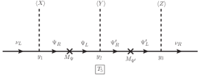
Figure 1: Feynman diagrams representing the five different topologies, $T_{1}$, $T_{2}$, $T_{3}$, $T_{4}$, $T_{5}$, respectively.

Each topology involves new “messenger fields” which can be either new scalars ($\varphi$), new fermions ($\Psi$) or both. The masses of these heavy messenger fields lying typically at or above the cutoff scale $\Lambda$ of the dimension-6 operators. The first topology $T_{1}$ involves two messenger fields, a scalar ($\varphi$) and a Dirac fermion ($\Psi$). The scalar $\varphi$ gets a small induced vev through its trilinear coupling with $Y$ and $Z$ scalars. Topology $T_{2}$ is very similar to $T_{1}$ and also involves two messenger fields, a scalar $\varphi$ and a Dirac fermion $\Psi$. However, the small vev of $\varphi$ in $T_{2}$ is induced by its trilinear coupling with $X$ and $Y$ scalars. The third topology $T_{3}$ is distinct from the first two and only involves scalar messengers $\varphi$ and $\varphi^{\prime}$. The scalar $\varphi^{\prime}$ gets a small induced vev through its trilinear coupling with $Y$ and $Z$ scalars. The other scalar $\varphi$ subsequently gets a “doubly-induced vev” through its trilinear coupling with $\varphi^{\prime}$ and $X$ scalars. The fourth topology $T_{4}$ only involves a single messenger scalar $\varphi$ which gets an induced vev through its quartic coupling with scalars $X$, $Y$ and $Z$. The final fifth topology involves only fermionic Dirac messengers $\Psi$ and $\Psi^{\prime}$, as shown in Fig. 1. The $SU(2)_{L}\otimes U(1)_{Y}$ charges of the messenger fields in all topologies will depend on the details of the operator under consideration and the contractions involved. We will discuss all such possibilities in the following sections. Each topology leads to different estimates for the associated light neutrino mass generated in each case, neglecting the three generation structure of the various Yukawa coupling matrices in family space. The resulting formulas for the neutrino masses are listed in Table 2.

Topology	Messenger Fields	Neutrino Mass Estimate
T1	$\Psi$, $\varphi$	$\frac{\mu y_{1}y_{2}\,v_{X}v_{Y}v_{Z}}{M_{\psi}M^{2}_{\varphi}}$
T2	$\Psi$, $\varphi$	$\frac{\mu y_{1}y_{2}\,v_{X}v_{Y}v_{Z}}{M_{\psi}M^{2}_{\varphi}}$
T3	$\varphi$, $\varphi^{\prime}$	$\frac{\mu_{1}\mu_{2}y\,v_{X}v_{Y}v_{Z}}{M^{2}_{\varphi}M^{2}_{\varphi^{\prime}}}$
T4	$\varphi$	$\frac{y\lambda\,v_{X}v_{Y}v_{Z}}{M^{2}_{\varphi}}$
T5	$\Psi$, $\Psi^{\prime}$	$\frac{y_{1}y_{2}y_{3}\,v_{X}v_{Y}v_{Z}}{M_{\psi}M_{\psi^{\prime}}}$

Table 2: Possible topologies and messengers leading to light neutrino masses, and the associated estimates for each topology.

Having discussed the various possible dimension-6 operators for Dirac neutrino mass generation and the various topologies involved in the UV- complete-models, in the following sections we discuss the various operators and topologies in more detail. To clarify the notation used in upcoming sections we list, as an illustration, all possible $SU(2)$ contractions of $\Phi$ and $\bar{\Phi}$ explicitly in Table 3.

Field 1	Field 2	Implicit contraction	Explicit contraction
$\Phi$	$\Phi$	$\underbrace{\Phi\otimes\Phi}_{1}$	$\Phi^{\alpha}\epsilon_{\alpha\beta}\Phi^{\beta}=0$
$\Phi$	$\bar{\Phi}$	$\underbrace{\Phi\otimes\bar{\Phi}}_{1}$	$\Phi^{\alpha}\delta_{\alpha}^{\beta}\Phi^{*}_{\beta}$
$\Phi$	$\Phi$	$\underbrace{\Phi\otimes\Phi}_{3}$	$\Phi^{\alpha}(\tau^{a})_{\alpha}^{\,\,\,\,\beta}\epsilon_{\beta\sigma}\Phi^{\sigma}$
$\Phi$	$\bar{\Phi}$	$\underbrace{\Phi\otimes\bar{\Phi}}_{3}$	$\Phi^{\alpha}(\tau^{a})_{\alpha}^{\,\,\,\,\beta}\Phi^{*}_{\beta}$
$\bar{\Phi}$	$\bar{\Phi}$	$\underbrace{\bar{\Phi}\otimes\bar{\Phi}}_{1}$	$\Phi^{*}_{\alpha}\epsilon^{\alpha\beta}\Phi^{*}_{\beta}=0$
$\bar{\Phi}$	$\bar{\Phi}$	$\underbrace{\bar{\Phi}\otimes\bar{\Phi}}_{3}$	$\Phi^{*}_{\alpha}\epsilon^{\alpha\sigma}(\tau^{a})_{\sigma}^{\,\,\,\,\beta}\Phi^{*}_{\beta}$

Table 3: The possible $SU(2)_{L}$ contractions of $\Phi$ and $\bar{\Phi}$, where $\tau^{a}=\tau^{+},\tau^{3},\tau^{-}$ are the three $SU(2)_{L}$ generators.

Similar notation will be used for contractions of other field multiplets in upcoming sections. For the sake of brevity we will not write them explicitly, though the contractions involved should be clear from the context. The UV-complete models arising from the operators listed in Table 1 will all involve certain new bosonic and/or fermionic messengers. These fields will be heavy, with masses close to the cutoff scale $\Lambda$. All relevant messenger fields will be singlet under $SU(3)_{C}$, while their transformation under $SU(2)_{L}\otimes U(1)_{Y}$ will vary. For quick reference we list all such messenger fields, their Lorentz transformation and $SU(2)_{L}$ and $U(1)_{Y}$ charges are given in the Table. 4. Everywhere, except for Standard Model fields, the subscript denotes the hypercharge. To make the notation lighter this is not done for Standard Model fields. In contrast to $\chi_{0}$, $\Phi$ and $\Delta_{i}$, which are the external scalars that acquire vevs, we denote as $\chi^{\prime}_{0}$ the messenger singlets which develop only an induced vev. The corresponding doublets will be denoted as $\sigma_{1}\equiv\Phi^{\prime}$ and the triplets are denoted as $\Delta_{i}^{\prime}$. The electric charge conservation implies that all the components appearing in the diagrams must be electrically neutral.

Messenger Field	Lorentz	$SU(2)_{L}$	$U(1)_{Y}$
$\chi^{\prime}_{0}$	Scalar	$1$	$0$
$N_{L,0},N_{R,0}$	Fermion	$1$	$0$
$\sigma_{1}$	Scalar	$2$	$1$
$E_{L,1},E_{R,1}$	Fermion	$2$	$1$
$E_{L,-1},E_{R,-1}$	Fermion	$2$	$-1$
$\Delta^{\prime}_{0}$	Scalar	$3$	$0$
$\Delta^{\prime}_{2}$	Scalar	$3$	$2$
$\Delta^{\prime}_{-2}$	Scalar	$3$	$-2$
$\Sigma_{L,0},\Sigma_{R,0}$	Fermion	$3$	$0$
$\Sigma_{L,2},\Sigma_{R,2}$	Fermion	$3$	$2$
$\Sigma_{L,-2},\Sigma_{R,-2}$	Fermion	$3$	$-2$
$\Xi_{1}$	Scalar	$4$	$1$
$Q_{L,-1},Q_{R,-1}$	Fermion	$4$	$-1$

Table 4: Messengers transform under $SU(2)_{L}$ and $U(1)_{Y}$ as given, they are color singlets and we are using the convention $Q=T_{3}+\frac{Y}{2}$. See text for the explanation of the notation used.

Note that certain messenger fields e.g $\Delta^{\prime}_{2}$ and $\Delta^{\prime}_{-2}$ are related with each other, for example $\bar{\Delta}^{\prime}_{2}\equiv\Delta^{\prime}_{-2}$. We have chosen to give them different symbols to avoid any confusion and also for aesthetics reasons. The notation and transformation properties of these messenger fields as listed in Table. 4 will be used throughout the rest of the paper.

III Operator Involving only the Standard Model Doublet

We begin our discussion with the operator involving only Standard Model scalar doublet $\Phi$ and discuss the various possible UV-complete models for this case. As has been argued in CentellesChulia:2018gwr , for Dirac neutrinos, after the Yukawa term, the lowest dimensional operator involving only the Standard Model scalar doublet appears at dimension-6 and is given by

$$\frac{1}{\Lambda^{2}}\bar{L}\otimes\bar{\Phi}\otimes\bar{\Phi}\otimes\Phi\otimes\nu_{R}$$ (2)

where $L$ and $\Phi$ denote the lepton and Higgs doublets, $\nu_{R}$ is the right-handed neutrino field and $\Lambda$ represents the cutoff scale. Above $\Lambda$ the Ultra-Violet (UV) complete theory is at play, involving new “messenger” fields, whose masses lie close to the scale $\Lambda$. Recently, this operator has also been studied in Yao:2017vtm and our results agree with those obtained in that work.

Before starting our systematic classification of the UV-complete seesaw models emerging from this operator, we stress that, in order for this operator to give the leading contribution to Dirac neutrino masses, the lower dimensional Yukawa term $\bar{L}\bar{\Phi}\nu_{R}$ should be forbidden. This can happen in many scenarios involving flavor symmetries Chulia:2016ngi ; Chulia:2016giq ; CentellesChulia:2017koy and/or additional $U(1)_{B-L}$ symmetries with unconventional charges for $\nu_{R}$ Ma:2014qra ; Ma:2015mjd . If this dimension-4 operator is forbidden by a simple $U(1)$ or $Z_{n}$ symmetry, then it is easy to see that the dimension-6 operator will also be forbidden. However, the dimension-4 operator can be forbidden in other ways. As a first possibility, one could have a softly broken symmetry, such as $Z_{3}$ Yao:2017vtm . Alternatively, one can add a new Higgs doublet $\Phi_{2}$ transforming as the Standard Model Higgs under the gauge group. One can show that, in such a two-doublet Higgs model (2HDM) the imposition of a $Z_{3}$ symmetry, under with the two Higgses transform non-trivially, is sufficient. The diagrams and discussion of this section will be identical for the 2HDM case, except that a label $\Phi_{1}$ or $\Phi_{2}$ should be added instead of simply $\Phi$. Finally, one may invoke non-abelian discrete symmetries such as $S_{4}$ Yao:2017vtm .

The operator in (2) can lead to several different UV-complete seesaw models, depending on the field contractions involved. There are fifteen inequivalent ways of contracting these fields, each of which will require different types of messenger fields for UV-completion. Out of these, one is similar to type I Dirac seesaw but with induced vev for the singlet scalar. Three of them are type-II-like, with induced vevs for the messenger scalars. Five of them are analogous to the three type-III Dirac seesaws discussed in CentellesChulia:2018gwr , with induced vevs for either the singlet or the triplet, while the other six are new diagrams. We now look at these possibilities one by one.

III.1 Type I seesaw mechanism with induced vev

One of the simplest contractions for the dimension-6 operator of (2) is as follows:

$$\underbrace{\underbrace{\underbrace{\bar{L}\otimes\bar{\Phi}}_{1}\otimes\underbrace{\bar{\Phi}\otimes\Phi}_{1}}_{1}\otimes\underbrace{\nu_{R}}_{1}}_{\textnormal{Type I with induced vev Fig.\leavevmode\nobreak\ \ref{DT1}}}$$ (3)

In (3) the under-brace denotes a $SU(2)_{L}$ contraction of the fields involved, whereas the number given under it denotes the transformation of the contracted fields under $SU(2)_{L}$ (note that the other possible contraction in which $\bar{\Phi}\otimes\bar{\Phi}$ goes to a singlet is simply $0$). Although not made explicit, we take it for granted that the global contraction leading to a UV-complete model where the neutrino mass is generated by the diagram shown in Fig. 2 should always be an $SU(2)_{L}$ singlet.

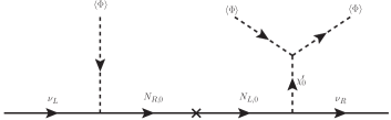
Figure 2: Feynman diagram representing the Dirac Type-I seesaw with an induced vev for $\chi^{\prime}_{0}$.

The diagram in Fig. 2 belongs to the topology $T_{1}$ and involves two messenger fields, a vector-like neutral fermion $N_{0}$ and a scalar $\chi^{\prime}_{0}$, both of which are singlet under the $\mathrm{SU(3)_{C}\otimes SU(2)_{L}\otimes U(1)_{Y}}$ gauge group. As listed in Table 2, the light neutrino mass is doubly suppressed first by the mass of the fermion $N_{0}$ and also by the small induced vev for $\chi^{\prime}_{0}$. In contrast to the type I Dirac seesaw diagram of Ref. CentellesChulia:2018gwr , here the messenger field $\chi^{\prime}_{0}$ required for the UV-completion gets a small induced vev via its cubic coupling with the Standard Model Higgs doublet.

III.2 Type II seesaw mechanism with induced vev

The three possibilities for this case are shown in (4).

$$\underbrace{\underbrace{\underbrace{\bar{L}\otimes\nu_{R}}_{2}\otimes\underbrace{\bar{\Phi}\otimes\Phi}_{1}}_{2}\otimes\underbrace{\bar{\Phi}}_{2}}_{\textnormal{Type II with induced vev Fig.\leavevmode\nobreak\ \ref{DT2}}},\hskip 14.22636pt\underbrace{\underbrace{\underbrace{\bar{L}\otimes\nu_{R}}_{2}\otimes\underbrace{\bar{\Phi}\otimes\Phi}_{3}}_{2}\otimes\underbrace{\bar{\Phi}}_{2}}_{\textnormal{Type II with induced vev Fig.\leavevmode\nobreak\ \ref{DT2}}},\hskip 14.22636pt\underbrace{\underbrace{\underbrace{\bar{L}\otimes\nu_{R}}_{2}\otimes\underbrace{\bar{\Phi}\otimes\bar{\Phi}_{3}}_{2}}\otimes\underbrace{\Phi}_{2}}_{\textnormal{Type II with induced vev Fig.\leavevmode\nobreak\ \ref{DT2}}}$$ (4)

These three contraction possibilities lead to three different UV-completions, as illustrated in Fig. 3.

,    ,    ,

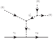
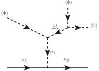
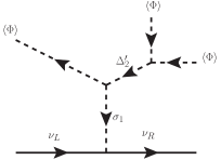
Figure 3: Feynman diagrams representing the three realizations of the Dirac Type-II seesaw with an induced vev for $\chi^{\prime}_{0}$ or $\Delta^{\prime}_{i}$.

All diagrams in Fig. 3 belong to the $T_{3}$ topology, and require two scalar messengers. The diagram on the left requires a $SU(2)_{L}$ singlet $\chi^{\prime}_{0}$ and a new doublet $\sigma_{1}$ (different from the Standard Model Higgs doublet) with $U(1)_{Y}=1$. The middle one requires an $SU(2)_{L}$ triplet $\Delta^{\prime}_{0}$ (with $U(1)_{Y}=0$) and an $SU(2)_{L}$ doublet $\sigma_{1}$ (with $U(1)_{Y}=1$) scalar messengers. The third diagram is identical to the second, exchanging $\Phi\leftrightarrow\bar{\Phi}$ in two external legs. Note that the hypercharges of the intermediate fields $\Delta^{\prime}_{0}$ and $\Delta^{\prime}_{2}$ are different so that, although the UV-completions share the same topology, the underlying models are different. The associated light neutrino mass estimate is given in Table 2.

III.3 Type III seesaw mechanism with induced vevs

The operator of (2) also leads to five distinct type-III like seesaw possibilities with induced vevs . The various possible contractions leading to such possibilities as shown in (5).

$$\underbrace{\underbrace{\underbrace{\bar{L}}_{2}\otimes\underbrace{\bar{\Phi}\otimes\Phi}_{1}}_{2}\otimes\underbrace{\bar{\Phi}\otimes\nu_{R}}_{2}}_{\textnormal{Type III with induced vev Fig.\leavevmode\nobreak\ \ref{DT3}}},\hskip 14.22636pt\underbrace{\underbrace{\underbrace{\bar{L}}_{2}\otimes\underbrace{\bar{\Phi}\otimes\Phi}_{3}}_{2}\otimes\underbrace{\bar{\Phi}\otimes\nu_{R}}_{2}}_{\textnormal{Type III with induced vev Fig.\leavevmode\nobreak\ \ref{DT3}}},\hskip 14.22636pt\underbrace{\underbrace{\underbrace{\bar{L}}_{2}\otimes\underbrace{\bar{\Phi}\otimes\bar{\Phi}}_{3}}_{2}\otimes\underbrace{{\Phi}\otimes\nu_{R}}_{2}}_{\textnormal{Type III with induced vev Fig.\leavevmode\nobreak\ \ref{DT3}}}$$

$$\underbrace{\underbrace{\underbrace{\bar{L}\otimes\bar{\Phi}}_{3}\otimes\underbrace{\bar{\Phi}\otimes\Phi}_{3}}_{1}\otimes\underbrace{\nu_{R}}_{1}}_{\textnormal{Type III with induced vev Fig.\leavevmode\nobreak\ \ref{DT3}}},\hskip 14.22636pt\underbrace{\underbrace{\underbrace{\bar{L}\otimes{\Phi}}_{3}\otimes\underbrace{\bar{\Phi}\otimes\bar{\Phi}}_{3}}_{1}\otimes\underbrace{\nu_{R}}_{1}}_{\textnormal{Type III with induced vev Fig.\leavevmode\nobreak\ \ref{DT3}}}$$ (5)

The UV-completions of each of these possible contractions involve different messenger fields, leading to five inequivalent models. The neutrino mass generation in these models is shown diagrammatically in Figure 4.

,    ,    ,    ,   

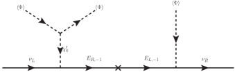
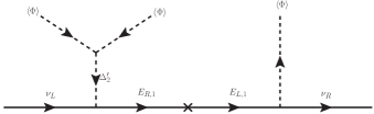
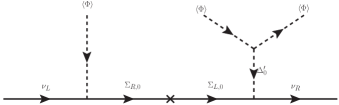
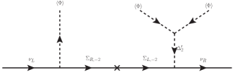
Figure 4: Feynman diagram representing the five realizations of the Dirac Type-III seesaw with an induced vev for $\chi^{\prime}_{0}$ or $\Delta^{\prime}_{i}$.

The first diagram in Figure 4 involves, as messenger fields, scalar singlet $\chi^{\prime}_{0}$ and vector-like fermions $E_{-1}$ transforming as an $SU(2)_{L}$ doublet with $U(1)_{Y}=-1$. The second diagram involves hypercharge-less $SU(2)_{L}$ triplet scalars $\Delta^{\prime}_{0}$ and the same $SU(2)_{L}$ doublet vector-like fermion $E_{-1}$ as messenger fields. The third diagram is identical to the second one, but with exchange $\Phi\leftrightarrow\bar{\Phi}$ in the external legs. This leads to a different hypercharge $U(1)_{Y}=2$ for the intermediate scalar triplet $\Delta^{\prime}_{2}$, as well as for the $SU(2)_{L}$ doublet vector fermion $E_{1}$, with $U(1)_{Y}=1$. The fourth and fifth diagrams again are related to each other by exchanging $\Phi\leftrightarrow\bar{\Phi}$ in two external legs. They involve, as messenger fields, $SU(2)_{L}$ triplet scalars $\Delta^{\prime}_{i}$; $i=0,2$ together with vector-like $SU(2)_{L}$ triplet fermions $\Sigma_{i}$; $i=0,-2$. The hypercharges of $\Delta_{i}^{\prime}$ are $U(1)_{Y}=0,2$ and of $\Sigma_{i}$ are $U(1)_{Y}=0,-2$ respectively. The first three diagrams belong to $T_{2}$ topology, while the fourth and fifth diagrams have the topology $T_{1}$ and the associated light neutrino masses for $T_{1}$ and $T_{2}$ are given in Table 2. Notice that, in contrast to the type III like Dirac seesaw diagrams discussed in CentellesChulia:2018gwr , here the $\chi^{\prime}_{0}$ and $\Delta^{\prime}_{i}$ both get induced vevs from their cubic interaction terms with the Standard Model Higgs doublet.

III.4 New diagrams

Apart from the above diagrams, there are also six new ones which have no dimension-5 analogues listed in Ref. CentellesChulia:2018gwr . The first of these possibilities arise from the field contraction shown in (6).

$$\underbrace{\underbrace{\bar{L}\otimes\nu_{R}}_{2}\otimes\underbrace{\bar{\Phi}\otimes\Phi\otimes\bar{\Phi}}_{2}}_{\textnormal{Fig. \ref{DT2new}}},\hskip 14.22636pt$$ (6)

This particular contraction of the operators leads to a UV-complete model where the neutrino mass arises from the Feynman diagram shown in Fig. 5 involving a single scalar messenger field $\sigma_{1}$ transforming as $SU(2)_{L}$ doublet with $U(1)_{Y}=1$.

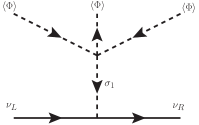
Figure 5: Feynman diagram representing the new possible UV completion belonging to topology $T_{4}$.

The field $\sigma_{1}$ gets a small induced vev through its quartic coupling with the Standard Model Higgs doublet. This diagram belongs to the $T_{4}$ topology and the resulting light neutrino mass estimate is given in Table 2.

Finally, there are five other field contractions of the dimension-6 operator, as shown in (7) and (8).

$$\underbrace{\underbrace{\underbrace{\bar{L}\otimes\bar{\Phi}}_{1}\otimes\underbrace{\bar{\Phi}}_{2}}_{2}\otimes\underbrace{\Phi\otimes\nu_{R}}_{2}}_{\textnormal{Fig. \ref{DN1}}},\hskip 14.22636pt\underbrace{\underbrace{\underbrace{\bar{L}\otimes\bar{\Phi}}_{1}\otimes\underbrace{\Phi}_{2}}_{2}\otimes\underbrace{\bar{\Phi}\otimes\nu_{R}}_{2}}_{\textnormal{Fig. \ref{DN1}}}$$ (7)

$$\underbrace{\underbrace{\underbrace{\bar{L}\otimes\bar{\Phi}}_{3}\otimes\underbrace{\bar{\Phi}}_{2}}_{2}\otimes\underbrace{\Phi\otimes\nu_{R}}_{2}}_{\textnormal{Fig. \ref{DN1}}},\hskip 14.22636pt\underbrace{\underbrace{\underbrace{\bar{L}\otimes\bar{\Phi}}_{3}\otimes\underbrace{\Phi}_{2}}_{2}\otimes\underbrace{\bar{\Phi}\otimes\nu_{R}}_{2}}_{\textnormal{Fig. \ref{DN1}}},\hskip 14.22636pt\underbrace{\underbrace{\underbrace{\bar{L}\otimes\Phi}_{3}\otimes\underbrace{\bar{\Phi}}_{2}}_{2}\otimes\underbrace{\bar{\Phi}\otimes\nu_{R}}_{2}}_{\textnormal{Fig. \ref{DN1}}}$$ (8)

Notice that the UV-completions of these five field contractions lead to the neutrino mass generation through topology $T_{5}$ , as shown diagrammatically in Fig. 6.

,    ,
,    ,   

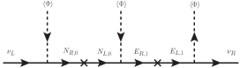
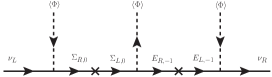
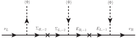
Figure 6: Feynman diagram representing the five realizations of the topology $T_{5}$ diagrams.

All these UV complete models only involve fermionic messengers. One sees that two different types of fermionic messengers are needed. In the first and second diagrams the $N_{0}$ is a vector-like gauge singlet fermion, whereas the vector fermions $E_{1}$ or $E_{-1}$ are $SU(2)_{L}$ doublets. In the first diagram the field $E_{1}$ carries a hypercharge $U(1)_{Y}=1$ while in the second diagram $E_{-1}$ carries a hypercharge $U(1)_{Y}=-1$. The last three diagrams in Fig. 6 also involve two types of fermionic messengers the vector-like fermions $E_{1}$ or $E_{-1}$ are $SU(2)_{L}$ doublets, while the vector-like fermions $\Sigma_{i}$ transform as triplet under the $SU(2)_{L}$ symmetry. In the third diagram $\Sigma_{0}$ carries no hypercharge while $E_{1}$ has $U(1)_{Y}=1$. In the fourth diagram $\Sigma_{0}$ carries no hypercharge, but $E_{-1}$ has $U(1)_{Y}=-1$. In the fifth diagram $\Sigma_{-2}$ has hypercharge $U(1)_{Y}=-2$, while $E_{-1}$ again has $U(1)_{Y}=-1$. The light neutrino mass expected for all these diagrams is the same as that given in Table 2 for $T_{5}$ topology.

IV Operators Involving Only Singlet ($\chi$) and Doublet ($\Phi$)

Having discussed the dimension-6 operator involving only the Standard Model Higgs doublet, we now move on to discuss other dimension-6 operators listed in Table 1 and their UV completions. We start our discussion with the relatively simpler operator $\bar{L}\otimes\chi_{0}\otimes\chi_{0}\otimes\bar{\Phi}\otimes\nu_{R}$ which, apart from the Standard Model Higgs doublet $\Phi$, also has a vev carrying singlet $\chi_{0}$. It is clear that the $\chi_{0}$ should not carry any $U(1)_{Y}$ charge, otherwise its vev will spontaneously break the electric charge conservation.

If $\chi_{0}$ is a complex field then, apart from h.c. of above operator, one can also write down two other operators namely $\bar{L}\otimes\bar{\chi_{0}}\otimes\bar{\chi_{0}}\otimes\bar{\Phi}\otimes\nu_{R}$ and $\bar{L}\otimes\bar{\chi_{0}}\otimes\chi_{0}\otimes\bar{\Phi}\otimes\nu_{R}$. In this section we will focus on the $\bar{L}\otimes\chi_{0}\otimes\chi_{0}\otimes\bar{\Phi}\otimes\nu_{R}$ case, since the other operator contractions and UV-completions are very similar and can be treated analogously. The operator $\bar{L}\otimes\chi_{0}\otimes\chi_{0}\otimes\bar{\Phi}\otimes\nu_{R}$ will give the leading contribution to neutrino masses only if similar operators of equal or lower dimensionality are forbidden by some symmetry. Thus lower dimensional operators allowed by $SU(2)_{L}\otimes U(1)_{Y}$ gauge symmetry, such as $\bar{L}\bar{\Phi}\nu_{R}$, $\bar{L}\bar{\Phi}\chi_{0}\nu_{R}$ and $\bar{L}\bar{\Phi}\bar{\chi_{0}}\nu_{R}$, should be forbidden. It is also desirable that this operator provides the sole contribution to neutrino masses, avoiding other dimension-6 operators such as $\bar{L}\bar{\Phi}\bar{\Phi}\Phi\nu_{R}$. A consistent scenario can arise in many ways with different symmetries. For example one of the simplest symmetries can be a $Z_{4}$ symmetry (distinct from quarticity symmetry) under which the fields transform as

$$\bar{L}\otimes\nu_{R}\sim z^{2},\hskip 5.69054pt\chi_{0}\sim z,\hskip 5.69054pt\Phi\sim 1,$$ (9)

Note that under these charge assignments the operator $\bar{L}\otimes\bar{\chi_{0}}\otimes\chi_{0}\otimes\bar{\Phi}\otimes\nu_{R}$ is forbidden though both $\bar{L}\otimes\chi_{0}\otimes\chi_{0}\otimes\bar{\Phi}\otimes\nu_{R}$ and $\bar{L}\otimes\bar{\chi_{0}}\otimes\bar{\chi_{0}}\otimes\bar{\Phi}\otimes\nu_{R}$ are allowed. Hence, in principle they can simultaneously contribute to neutrino mass generation, as long as they have consistent UV-completions. Here we will only discuss the first operator, though the other may be present in some cases. Moreover, note that the masses of charged leptons and quarks can be generated through the usual Yukawa terms, i.e. $\bar{L}\Phi l_{R}$, $\bar{Q}\Phi d_{R}$ and $\bar{Q}\bar{\Phi}u_{R}$ can be trivially allowed by this symmetry with appropriate $Z_{4}$ charges of $Q$, $l_{R}$, $u_{R}$ and $d_{R}$.

Moving on to the operator contractions and UV completions, there are ten different ways of contracting this operator. Each of the topologies $T_{1}$, $T_{2}$ and $T_{3}$ appears twice, while one diagram belongs to the $T_{4}$ topology and the three others belong to the $T_{5}$ topology. The operator contractions which lead to diagrams with $T_{1}$ or $T_{2}$ topologies are listed in (10), and the corresponding diagrams are shown in Fig. 7.

$$\underbrace{\underbrace{\bar{L}\otimes\chi_{0}}_{2}\otimes\underbrace{\bar{\Phi}\otimes\chi_{0}}_{2}}_{1}\otimes\underbrace{\nu_{R}}_{1},\hskip 14.22636pt\underbrace{\underbrace{\bar{L}\otimes\bar{\Phi}}_{1}\otimes\underbrace{\chi_{0}\otimes\chi_{0}}_{1}}_{1}\otimes\underbrace{\nu_{R}}_{1},\hskip 14.22636pt\underbrace{\underbrace{\bar{L}}_{2}\otimes\underbrace{\chi_{0}\otimes\chi_{0}}_{1}}_{2}\otimes\underbrace{\bar{\Phi}\otimes\nu_{R}}_{2},\hskip 14.22636pt\underbrace{\underbrace{\bar{L}}_{2}\otimes\underbrace{\bar{\Phi}\otimes\chi_{0}}_{2}}_{1}\otimes\underbrace{\chi_{0}\otimes\nu_{R}}_{1}$$ (10)

,    ,    ,   

Figure 7: Diagrams showing the $T_{1}$ and $T_{2}$ topologies of the operator $\bar{L}\chi_{0}\chi_{0}\bar{\Phi}\nu_{R}$

As before, the UV completion of these diagrams will involve new messenger fields. In all of the cases shown in Fig. 7 there is a scalar ($\chi_{0}^{\prime}$ or $\sigma_{1}$) and a vector-like lepton ($N_{0}$ or $E_{i}$) messenger involved. Notice that $\chi^{\prime}_{0}$ cannot be identified with $\chi_{0}$ as in that case lower dimension-5 operators would be allowed. Thus, they must carry different charges under the symmetry forbidding lower dimensional operators (e.g $Z_{4}$ mentioned above).

UV-completion lead to other possible contractions with the $T_{3}$ and $T_{4}$ topology, as shown in Fig. 8.

$$\underbrace{\underbrace{\bar{L}\otimes\nu_{R}}_{2}\otimes\underbrace{\chi_{0}}_{1}}_{2}\otimes\underbrace{\chi_{0}\otimes\bar{\Phi}}_{2},\hskip 14.22636pt\underbrace{\underbrace{\bar{L}\otimes\nu_{R}}_{2}\otimes\underbrace{\bar{\Phi}}_{2}}_{1}\otimes\underbrace{\chi_{0}\otimes\chi_{0}}_{1},\hskip 14.22636pt\underbrace{\underbrace{\bar{L}\otimes\nu_{R}}_{2}\otimes\underbrace{\bar{\Phi}\otimes\chi_{0}\otimes\chi_{0}}_{2}}_{1}$$ (11)

,    ,   

Figure 8: Diagrams showing the $T_{3}$ and $T_{4}$ topologies of the operator $\bar{L}\chi_{0}\chi_{0}\bar{\Phi}\nu_{R}$

All the three diagrams in Fig. 8 involve only scalar messenger fields which can be either $\chi^{\prime}_{0}$ or $\sigma_{1}$. The last diagram was realized in the Diracon model of Ref. Bonilla:2016zef . Notice that in the first diagram the messengers $\sigma_{1}$ and $\sigma_{1}^{\prime}$ must be different fields, since they will transform differently under the symmetry forbidding lower dimensional operators (e.g $Z_{4}$ of (9)). Likewise, $\chi^{\prime}_{0}$ has to be distinct from $\chi_{0}$ and $\sigma_{1}$ and $\sigma_{1}^{\prime}$ must be different from $\Phi$.

Finally three other possible contractions lead to the $T_{5}$-type UV-completion. These diagrams are shown in Fig. 9.

$$\underbrace{\underbrace{\bar{L}\otimes\bar{\Phi}}_{1}\otimes\underbrace{\chi_{0}}_{1}}_{1}\otimes\underbrace{\chi_{0}\otimes\nu_{R}}_{1},\hskip 14.22636pt\underbrace{\underbrace{\bar{L}\otimes\chi_{0}}_{2}\otimes\underbrace{\bar{\Phi}}_{2}}_{1}\otimes\underbrace{\chi_{0}\otimes\nu_{R}}_{1},\hskip 14.22636pt\underbrace{\underbrace{\bar{L}\otimes\chi_{0}}_{2}\otimes\underbrace{\chi_{0}}_{1}}_{2}\otimes\underbrace{\bar{\Phi}\otimes\nu_{R}}_{2}$$ (12)

,    ,   

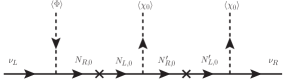
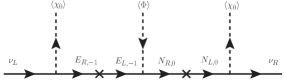
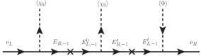
Figure 9: Diagrams showing the $T_{5}$ topology of the operator $\bar{L}\chi_{0}\chi_{0}\bar{\Phi}\nu_{R}$

All of the diagrams in Fig. 9 involve only fermionic messengers $N_{L,R}$ or $E_{L,R}$. Again, note that the fields $N_{0}$ and $N_{0}^{\prime}$ in the first diagram and the fields $E_{-1}$ and $E^{\prime}_{-1}$ in the third diagram must be different fields, since they transform differently under the symmetry forbidding lower dimensional operators (e.g $Z_{4}$ of (9)).

Before closing the section, let us briefly discuss the operator $\bar{L}\otimes\bar{\chi_{0}}\otimes\chi_{0}\otimes\bar{\Phi}\otimes\nu_{R}$. In addition to diagrams analogous to those above, there will be five other diagrams, as noted in Table 1. These new diagrams appear because, under the symmetry forbidding lower dimensional operators, $\chi_{0}$ and $\bar{\chi_{0}}$ transform differently so that the exchange $\chi_{0}\leftrightarrow\bar{\chi_{0}}$ leads to distinct UV completions. Finally, also for this operator, lower dimensional operators cannot be forbidden by simple $U(1)$ or $Z_{n}$ symmetries. More involved symmetries similar to those discussed in Section III would be needed. Alternatively, similar to the discussion in Section III, one may introduce two different singlet scalar fields $\chi^{(1)}_{0}$ and $\chi^{(2)}_{0}$ transforming differently under a $Z_{n}$ symmetry.

V Operators Involving Singlet ($\chi$), Doublet ($\Phi$) and Triplet ($\Delta$)

For this class of operators, there are two $U(1)_{Y}$ possibilities for scalar field $\Delta$. One is the operator $\bar{L}\otimes\chi_{0}\otimes\Phi\otimes\Delta_{-2}\otimes\nu_{R}$, in which $\Delta_{-2}\sim-2$ under $U(1)_{Y}$, while the other possibility is $\bar{L}\otimes\chi_{0}\otimes\bar{\Phi}\otimes\Delta_{0}\otimes\nu_{R}$ with $\Delta_{0}\sim 0$ under $U(1)_{Y}$. Apart from hermitian conjugation, one can also write down several other operators by replacing one or more of $\chi_{0},\Phi,\Delta_{i}$ by $\bar{\chi_{0}},\bar{\Phi},\bar{\Delta}_{i}$ respectively. Since the operator contractions and UV completion of these operators are all very similar, in this section we will primarily focus on $\bar{L}\otimes\chi_{0}\otimes\bar{\Phi}\otimes\Delta_{0}\otimes\nu_{R}$ operator. We will also comment on the changes required for the operator $\bar{L}\otimes\chi_{0}\otimes\Phi\otimes\Delta_{-2}\otimes\nu_{R}$. The discussion here will equally apply to the other operators which can be treated analogously.

As before, in order to ensure that this operator gives the leading contribution to neutrino masses we need extra symmetries. For the case of the operator $\bar{L}\chi_{0}\bar{\Phi}\Delta_{0}\nu_{R}$, due to the zero hypercharge of $\Delta_{0}$ there are many operators to forbid, so that $Z_{4}$ will not be enough, although a $Z_{6}$ can work with the charge assignments shown in 13.

$$\bar{L}\otimes\nu_{R}\sim\lambda^{3},\hskip 5.69054pt\Phi\sim 1,\hskip 5.69054pt\chi_{0}\sim\lambda^{2},\hskip 5.69054pt\Delta_{0}\sim\lambda$$ (13)

where $\lambda^{6}=1$. Note that these charge assignments forbid the $SU(2)_{L}\otimes U(1)_{Y}$ allowed operators $\bar{L}\bar{\Phi}\nu_{R}$, $\bar{L}\bar{\Phi}\bar{\Phi}\Phi\nu_{R}$, $\bar{L}\chi_{0}\chi_{0}\bar{\Phi}\nu_{R}$, $\bar{L}\chi_{0}^{\dagger}\chi_{0}\bar{\Phi}\nu_{R}$, $\bar{L}\chi_{0}^{\dagger}\chi_{0}^{\dagger}\bar{\Phi}\nu_{R}$, $\bar{L}\Delta\Delta\bar{\Phi}\nu_{R}$, $\bar{L}\Delta^{\dagger}\Delta\bar{\Phi}\nu_{R}$, $\bar{L}\Delta^{\dagger}\Delta^{\dagger}\bar{\Phi}\nu_{R}$, $\bar{L}\chi_{0}\bar{\Phi}\nu_{R}$, $\bar{L}\chi_{0}^{\dagger}\bar{\Phi}\nu_{R}$ and $\bar{L}\Delta\Phi\nu_{R}$.

For the other $U(1)_{Y}$ allowed operator $\bar{L}\chi_{0}\Phi\Delta_{-2}\nu_{R}$, the minimal symmetry that works is another $Z_{4}$, under which the charges of particles are given in Eq. 14.

$$\bar{L}\otimes\nu_{R}\sim z,\hskip 5.69054pt\Phi\sim 1,\hskip 5.69054pt\chi_{0}\sim z^{2},\hskip 5.69054pt\Delta_{-2}\sim z$$ (14)

This charge assignment will forbid operators such as $\bar{L}\bar{\Phi}\nu_{R}$, $\bar{L}\bar{\Phi}\bar{\Phi}\Phi\nu_{R}$, $\bar{L}\chi_{0}\chi_{0}\bar{\Phi}\nu_{R}$, $\bar{L}\chi_{0}^{\dagger}\chi_{0}\bar{\Phi}\nu_{R}$, $\bar{L}\chi_{0}^{\dagger}\chi_{0}^{\dagger}\bar{\Phi}\nu_{R}$, $\bar{L}\Delta^{\dagger}\Delta\bar{\Phi}\nu_{R}$, $\bar{L}\chi_{0}\bar{\Phi}\nu_{R}$ and $\bar{L}\chi_{0}^{\dagger}\bar{\Phi}\nu_{R}$ and $\bar{L}\Delta\Phi\nu_{R}$.

Note that Yukawa terms for other Standard Model fermions, i.e. $\bar{L}\Phi l_{R}$, $\bar{Q}\Phi d_{R}$ and $\bar{Q}\bar{\Phi}u_{R}$ can be trivially allowed by these symmetries with appropriate $Z_{4}$ or $Z_{6}$ charges of $\bar{Q}$, $l_{R}$, $u_{R}$ and $d_{R}$].

It is easy to see that with this charge assignment, all unwanted operators will be forbidden. We stress that the above two symmetries are given just for illustration. The unwanted operators can be forbidden in many other ways.

As mentioned before, for sake of brevity we will only explicitly discuss the case of $\bar{L}\otimes\chi_{0}\otimes\bar{\Phi}\otimes\Delta_{0}\otimes\nu_{R}$ operator. The diagrams and topologies of the $\bar{L}\otimes\chi_{0}\otimes\Phi\otimes\Delta_{-2}\otimes\nu_{R}$ operator will be quite similar and can be obtained from the $\Delta_{0}$ case by just changing the direction of the arrow and the $U(1)_{Y}$ charges of the intermediate messenger fields. The diagrams for the other operators mentioned before can also be obtained in a similar manner.

Moving on to the possible operator contractions and UV-completions, here we have now sixteen possibilities. Three diagrams in each topologies $T_{1}$, $T_{2}$ and $T_{3}$, plus a diagram in $T_{4}$ and the remaining six diagrams in $T_{5}$ topology.

The three operator contractions which lead to diagrams with $T_{1}$ topology are given in (15) and their the UV complete diagrams are shown in Fig. 10.

$$\underbrace{\underbrace{\bar{L}\otimes\chi_{0}}_{2}\otimes\underbrace{\bar{\Phi}\otimes\Delta_{0}}_{2}}_{1}\otimes\underbrace{\nu_{R}}_{1},\hskip 14.22636pt\underbrace{\underbrace{\bar{L}\otimes\bar{\Phi}}_{3}\otimes\underbrace{\chi_{0}\otimes\Delta_{0}}_{3}}_{1}\otimes\underbrace{\nu_{R}}_{1},\hskip 14.22636pt\underbrace{\underbrace{\bar{L}\otimes\Delta_{0}}_{2}\otimes\underbrace{\chi_{0}\otimes\bar{\Phi}}_{2}}_{1}\otimes\underbrace{\nu_{R}}_{1}$$ (15)

,    ,   

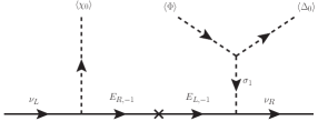
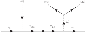
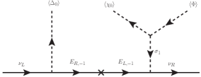
Figure 10: Diagrams associated to the $T_{1}$ topology of the operator $\bar{L}\chi_{0}\bar{\Phi}\Delta_{0}\nu_{R}$. Note that for the other choice of $U(1)_{Y}$, i.e. the operator $\bar{L}\chi_{0}\Phi\Delta_{-2}\nu_{R}$, the only difference in the diagrams will be flipping the direction of the arrow of the external $\Phi$ and $\Delta_{0}$.

Note that the first and third diagrams in Fig. 10 have the same field content and therefore coexist in the same model having this particle content unless a symmetry like the example symmetry in (13) forbids one of them.

The three operator contractions (16) and the corresponding diagrams for the $T_{2}$ topology are shown in Fig. 11.

$$\underbrace{\underbrace{\bar{L}}_{2}\otimes\underbrace{\chi_{0}\otimes\bar{\Phi}}_{2}}_{3}\otimes\underbrace{\Delta_{0}\otimes\nu_{R}}_{3},\hskip 14.22636pt\underbrace{\underbrace{\bar{L}}_{2}\otimes\underbrace{\chi_{0}\otimes\Delta_{0}}_{3}}_{2}\otimes\underbrace{\bar{\Phi}\otimes\nu_{R}}_{2},\hskip 14.22636pt\underbrace{\underbrace{\bar{L}}_{2}\otimes\underbrace{\bar{\Phi}\otimes\Delta_{0}}_{2}}_{1}\otimes\underbrace{\chi_{0}\otimes\nu_{R}}_{1}$$ (16)

,    ,   

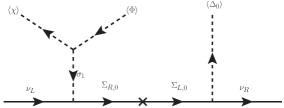
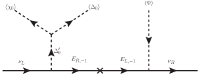
Figure 11: Diagrams showing the $T_{2}$ topology of the operator $\bar{L}\chi_{0}\bar{\Phi}\Delta_{0}\nu_{R}$. Note that the diagrams for operator $\bar{L}\chi_{0}\Phi\Delta_{-2}\nu_{R}$ can be obtained from these by flipping the direction of the arrow of the external $\Phi$ and $\Delta_{0}$ fields.

The contractions (17) and the UV-completions that lead to topologies $T_{3}$ or $T_{4}$ are shown in Fig. 12.

$$\underbrace{\underbrace{\bar{L}\otimes\nu_{R}}_{2}\otimes\underbrace{\chi_{0}}_{1}}_{2}\otimes\underbrace{\bar{\Phi}\otimes\Delta_{0}}_{2},\hskip 14.22636pt\underbrace{\underbrace{\bar{L}\otimes\nu_{R}}_{2}\otimes\underbrace{\Delta_{0}}_{3}}_{2}\otimes\underbrace{\chi_{0}\otimes\bar{\Phi}}_{2},\hskip 14.22636pt\underbrace{\underbrace{\bar{L}\otimes\nu_{R}}_{2}\otimes\underbrace{\bar{\Phi}}_{2}}_{3}\otimes\underbrace{\chi_{0}\otimes\Delta_{0}}_{3},\hskip 14.22636pt\underbrace{\bar{L}\otimes\nu_{R}}_{2}\otimes\underbrace{\chi_{0}\otimes\bar{\Phi}\otimes\Delta_{0}}_{2}$$ (17)

,    ,   
,   

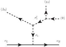
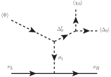
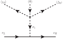
Figure 12: Diagrams showing the $T_{3}$ and $T_{4}$ topologies of the operator $\bar{L}\chi_{0}\bar{\Phi}\Delta_{0}\nu_{R}$. Note that the diagrams for operator $\bar{L}\chi_{0}{\Phi}\Delta_{-2}\nu_{R}$ can be obtained from these by flipping the direction of the arrow of the external $\Phi$ and $\Delta_{0}$ fields.

Again, we note that in Fig. 12 the first and second diagrams have the same field content. Therefore, in a typical model both diagrams will contribute to neutrino masses, unless one of them is explicitly forbidden by some symmetry.

Finally, there are six possible operator contractions leading to the $T_{5}$ topology, as shown in Fig. 13.

$$\underbrace{\underbrace{\bar{L}\otimes\chi_{0}}_{2}\otimes\underbrace{\bar{\Phi}}_{2}}_{3}\otimes\underbrace{\Delta_{0}\otimes\nu_{R}}_{3},\hskip 14.22636pt\underbrace{\underbrace{\bar{L}\otimes\chi_{0}}_{2}\otimes\underbrace{\Delta_{0}}_{3}}_{2}\otimes\underbrace{\bar{\Phi}\otimes\nu_{R}}_{2},\hskip 14.22636pt\underbrace{\underbrace{\bar{L}\otimes\bar{\Phi}}_{3}\otimes\underbrace{\chi_{0}}_{1}}_{3}\otimes\underbrace{\Delta_{0}\otimes\nu_{R}}_{3}$$ (18)

$$\underbrace{\underbrace{\bar{L}\otimes\bar{\Phi}}_{3}\otimes\underbrace{\Delta_{0}}_{3}}_{1}\otimes\underbrace{\chi_{0}\otimes\nu_{R}}_{1},\hskip 14.22636pt\underbrace{\underbrace{\bar{L}\otimes\Delta_{0}}_{2}\otimes\underbrace{\chi_{0}}_{1}}_{2}\otimes\underbrace{\bar{\Phi}\otimes\nu_{R}}_{2},\hskip 14.22636pt\underbrace{\underbrace{\bar{L}\otimes\Delta_{0}}_{2}\otimes\underbrace{\bar{\Phi}}_{2}}_{1}\otimes\underbrace{\chi_{0}\otimes\nu_{R}}_{1}$$ (19)

,    ,    ,    ,    ,   

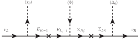
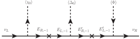
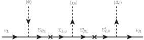
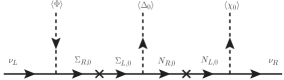
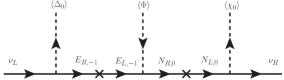
Figure 13: Diagrams showing the $T_{5}$ topology of the operator $\bar{L}\chi_{0}\bar{\Phi}\Delta_{0}\nu_{R}$. Note that the diagrams for operator $\bar{L}\chi_{0}\bar{\Phi}\Delta_{-2}\nu_{R}$ can be obtained from these by flipping the direction of the arrow of the external $\Phi$ and $\Delta_{0}$ fields.

Again note that, owing to their different transformation under symmetry forbidding lower dimensional operators, the fields $E_{-1}$ and $E^{\prime}_{-1}$ in the second and fifth diagrams of Fig. 13 must be different. Also, comparing these two diagrams one can see that they have the same messenger field content. However, these two diagrams belong to two distinct UV-complete models, due to the different charges of the messenger fields under symmetry forbidding lower dimensional operators. Hence they correspond to different models with the same field content.

VI Operators Involving Only Doublet ($\Phi$) and Triplet ($\Delta$)

There are several possibilities for dimension-6 operators involving $SU(2)_{L}$ doublet and triplet scalars, as listed in Table 1. As before, an extra symmetry is required in order to ensure that these operators give the leading contribution to neutrino masses. Again, the nature of this symmetry can vary from a simple $U(1)_{X}$ symmetry to its $Z_{n}$ subgroup, or more complex symmetries involving non-abelian groups. As discussed in Section II, depending on the symmetry required these operators can be classified into two categories (see Table 1) namely operators for which the lower dimensional operators can be forbidden by $U(1)_{X}$ or $Z_{n}$ symmetries and operators for which $U(1)_{X}$ or $Z_{n}$ symmetry is not enough.

For example the operators $\bar{L}\otimes\bar{\Phi}\otimes\Delta_{0}\otimes\Delta_{0}\otimes\nu_{R}$ and $\bar{L}\otimes\Phi\otimes\Delta_{0}\otimes\Delta_{-2}\otimes\nu_{R}$ can both be forbidden by a simple $Z_{n}$ symmetry. The minimal consistent one is a $Z_{4}$ symmetry, under which the various particles transform as

$$\bar{L}\otimes\nu_{R}\sim z^{2},\hskip 5.69054pt\Phi\sim 1,\hskip 5.69054pt\Delta_{i}\sim z$$ (20)

where $\Delta_{i}$, $i=0,-2$, denote the two different types of $SU(2)_{L}$ triplets. Note that under these charge assignments other operators where $\Delta_{0}\to\bar{\Delta}_{0}$ are also allowed and could in principle also contribute to neutrino masses, as long as they have consistent UV-completions. The other operators $\bar{L}\otimes\bar{\Phi}\otimes\bar{\Delta}_{i}\otimes\Delta_{i}\otimes\nu_{R}$; $i=0,-2$ belong to a different class and for such operators simple $U(1)_{X}$ or $Z_{n}$ symmetries are not enough to forbid all other dimension-6 and lower dimensional operators. Just as the case of $\bar{L}\otimes\bar{\Phi}\otimes\bar{\Phi}\otimes\Phi\otimes\nu_{R}$ operator discussed in Section III, these operators can also give leading contribution to neutrino masses through a softly broken $Z_{n}$ symmetry or for certain non-abelian discrete symmetries, such as $S_{4}$. Alternatively, for this case one may also introduce another copy of $\Delta_{i}$, in which case (as before) a simple $Z_{n}$ symmetry could suffice.

Moving on to possible operator contractions and UV-completions we first note that the UV-completions of all these operators are very similar to each other. To avoid unnecessary repetition we will only discuss in detail the UV-completion of the operator $\bar{L}\otimes\bar{\Phi}\otimes\bar{\Delta}_{0}\otimes\Delta_{0}\otimes\nu_{R}$. We have singled out this operator since, amongst all the operators of this category, it offers the maximum number of possible completions, see Table 1. The other operators can be treated in the same manner and we will comment on some of their salient features as we go along.

There are thirty one different ways of contracting this operator. Six digramas lie in each of the topologies $T_{1}$, $T_{2}$ and $T_{3}$. One belongs to $T_{4}$ topology, while the remaining twelve belong to $T_{5}$ topology.

The six operator contractions are given in (21), while their UV-complete diagrams are shown in Figure 14.

$$\underbrace{\underbrace{\bar{L}\otimes\bar{\Phi}}_{1}\otimes\underbrace{\bar{\Delta}_{0}\otimes\Delta_{0}}_{1}}_{1}\otimes\underbrace{\nu_{R}}_{1},\hskip 14.22636pt\underbrace{\underbrace{\bar{L}\otimes\bar{\Phi}}_{3}\otimes\underbrace{\bar{\Delta}_{0}\otimes\Delta_{0}}_{3}}_{1}\otimes\underbrace{\nu_{R}}_{1},\hskip 14.22636pt\underbrace{\underbrace{\bar{L}\otimes\bar{\Delta}_{0}}_{2}\otimes\underbrace{\Delta_{0}\otimes\bar{\Phi}}_{2}}_{1}\otimes\underbrace{\nu_{R}}_{1},\hskip 14.22636pt\underbrace{\underbrace{\bar{L}\otimes\Delta_{0}}_{2}\otimes\underbrace{\bar{\Delta}_{0}\otimes\bar{\Phi}}_{2}}_{1}\otimes\underbrace{\nu_{R}}_{1},$$

$$\underbrace{\underbrace{\bar{L}\otimes\bar{\Delta}_{0}}_{4}\otimes\underbrace{\Delta_{0}\otimes\bar{\Phi}}_{4}}_{1}\otimes\underbrace{\nu_{R}}_{1},\hskip 14.22636pt\underbrace{\underbrace{\bar{L}\otimes\Delta_{0}}_{4}\otimes\underbrace{\bar{\Delta}_{0}\otimes\bar{\Phi}}_{4}}_{1}\otimes\underbrace{\nu_{R}}_{1},\hskip 14.22636pt$$ (21)

,    ,    ,    ,    ,   

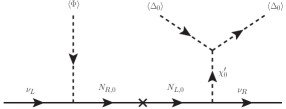
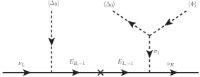
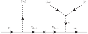
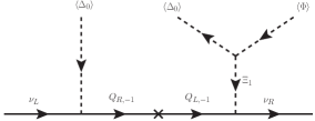
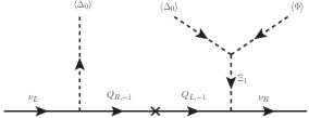
Figure 14: Diagrams showing the $T_{1}$ topology of the operator $\bar{L}\bar{\Phi}\bar{\Delta}_{0}\Delta_{0}\nu_{R}$.

Notice that the last two diagrams in Fig. 14 involve messengers transforming as quartets of $SU(2)_{L}$. The fermionic quartet $Q_{L,R}$ carry $U(1)_{Y}=-1$, while the scalar quartet $\Xi$ has $U(1)_{Y}=1$.

At this point we comment on the other operators mentioned in Table 1. For example, for the operator $\bar{L}\otimes\bar{\Phi}\otimes\bar{\Delta}_{-2}\otimes\Delta_{-2}\otimes\nu_{R}$ the third contraction of (21) will be forbidden, since it involves a contraction of $\bar{L}$ and $\bar{\Delta}_{-2}$ going to a doublet. This contraction implies that the resulting messenger will be an $SU(2)_{L}$ doublet with $U(1)_{Y}=3$. Hence it will not contribute to neutrino mass since it has no neutral component.

For the operator $\bar{L}\otimes\Phi\otimes\Delta_{0}\otimes\Delta_{-2}\otimes\nu_{R}$ the first contraction of (21) will have the same problem, namely the contraction of $\bar{L}$ with $\Phi$ implies an $SU(2)_{L}$ singlet messenger field with $U(1)_{Y}=-2$. For the operator $\bar{L}\otimes\bar{\Phi}\otimes\Delta_{0}\otimes\Delta_{0}\otimes\nu_{R}$, the second contraction of (21) will be forbidden, as in this case it involves a contraction of two identical triplets going to a triplet, which is zero. Moreover, for this case the third and fourth, as well as fifth and sixth contractions of (21) are identical to each other. Therefore only one diagram out of each pair should be counted for this case.

The six operator contractions which lead to $T_{2}$ topologies are given in (22). The corresponding diagrams are shown in Figure 15.

$$\underbrace{\underbrace{\bar{L}}_{2}\otimes\underbrace{\bar{\Delta}_{0}\otimes\Delta_{0}}_{1}}_{2}\otimes\underbrace{\bar{\Phi}\otimes\nu_{R}}_{2},\hskip 14.22636pt\underbrace{\underbrace{\bar{L}}_{2}\otimes\underbrace{\bar{\Delta}_{0}\otimes\Delta_{0}}_{3}}_{2}\otimes\underbrace{\bar{\Phi}\otimes\nu_{R}}_{2},\hskip 14.22636pt\underbrace{\underbrace{\bar{L}}_{2}\otimes\underbrace{\Delta_{0}\otimes\bar{\Phi}}_{2}}_{3}\otimes\underbrace{\bar{\Delta}_{0}\otimes\nu_{R}}_{3},\hskip 14.22636pt\underbrace{\underbrace{\bar{L}}_{2}\otimes\underbrace{\bar{\Delta}_{0}\otimes\bar{\Phi}}_{2}}_{3}\otimes\underbrace{\Delta_{0}\otimes\nu_{R}}_{3}$$

$$\underbrace{\underbrace{\bar{L}}_{2}\otimes\underbrace{\bar{\Delta}_{0}\otimes\bar{\Phi}}_{4}}_{3}\otimes\underbrace{\Delta_{0}\otimes\nu_{R}}_{3},\hskip 14.22636pt\underbrace{\underbrace{\bar{L}}_{2}\otimes\underbrace{\Delta_{0}\otimes\bar{\Phi}}_{4}}_{3}\otimes\underbrace{\bar{\Delta}_{0}\otimes\nu_{R}}_{3}$$ (22)

,    ,    ,    ,    ,   

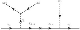
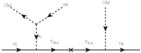
Figure 15: Diagrams showing the $T_{2}$ topology of the operator $\bar{L}\bar{\Phi}\bar{\Delta}_{0}\Delta_{0}\nu_{R}$.

Again notice the appearance of the scalar $SU(2)_{L}$ quartet $\Xi$ in the last two diagrams of Fig. 15. For the other operators listed in Table 1, some of the contractions in (22) are forbidden. For the operator $\bar{L}\otimes\bar{\Phi}\otimes\bar{\Delta}_{-2}\otimes\Delta_{-2}\otimes\nu_{R}$ the third contraction of (22) is forbidden as it implies a messenger doublet with $U(1)_{Y}=3$ which does not have a neutral component. For the operator $\bar{L}\otimes\Phi\otimes\Delta_{0}\otimes\Delta_{-2}\otimes\nu_{R}$ the first contraction of (22) leads to a singlet messenger with $U(1)_{Y}=-2$ and hence is forbidden. On the other hand, for the operator $\bar{L}\otimes\bar{\Phi}\otimes\Delta_{0}\otimes\Delta_{0}\otimes\nu_{R}$, the second contraction of (22) is forbidden, as it involves a contraction of two identical triplets going to a triplet, which is zero. Also, the third and fourth, as well as the fifth and sixth contractions are identical for this case. Therefore only one diagram out of each pair should be counted for this case.

The possible operator contractions leading to the $T_{3}$ and $T_{4}$ topologies are shown in (23) and in (24), while the corresponding diagrams are shown in Fig. 16.

$$\underbrace{\underbrace{\bar{L}\otimes\nu_{R}}_{2}\otimes\underbrace{\Delta_{0}}_{3}}_{2}\otimes\underbrace{\bar{\Phi}\otimes\bar{\Delta}_{0}}_{2},\hskip 14.22636pt\underbrace{\underbrace{\bar{L}\otimes\nu_{R}}_{2}\otimes\underbrace{\bar{\Delta}_{0}}_{3}}_{2}\otimes\underbrace{\bar{\Phi}\otimes\Delta_{0}}_{2},\hskip 14.22636pt\underbrace{\underbrace{\bar{L}\otimes\nu_{R}}_{2}\otimes\underbrace{\bar{\Phi}}_{2}}_{1}\otimes\underbrace{\bar{\Delta}_{0}\otimes\Delta_{0}}_{1},\hskip 14.22636pt\underbrace{\underbrace{\bar{L}\otimes\nu_{R}}_{2}\otimes\underbrace{\bar{\Phi}}_{2}}_{3}\otimes\underbrace{\bar{\Delta}_{0}\otimes\Delta_{0}}_{3}$$ (23)

$$\underbrace{\underbrace{\bar{L}\otimes\nu_{R}}_{2}\otimes\underbrace{\bar{\Delta}_{0}}_{3}}_{4}\otimes\underbrace{\bar{\Phi}\otimes\Delta_{0}}_{4},\hskip 14.22636pt\underbrace{\underbrace{\bar{L}\otimes\nu_{R}}_{2}\otimes\underbrace{\Delta_{0}}_{3}}_{4}\otimes\underbrace{\bar{\Phi}\otimes\bar{\Delta}_{0}}_{4},\hskip 14.22636pt\underbrace{\bar{L}\otimes\nu_{R}}_{2}\otimes\underbrace{\bar{\Delta}_{0}\otimes\bar{\Phi}\otimes\Delta_{0}}_{2}$$ (24)

,    ,   
,    ,    ,    ,   

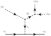
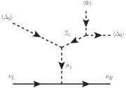
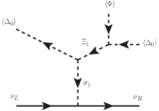
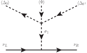
Figure 16: Diagrams showing the $T_{3}$ and $T_{4}$ topologies of the operator $\bar{L}\bar{\Phi}\bar{\Delta}_{0}\Delta_{0}\nu_{R}$.

Notice the appearance of the scalar $SU(2)_{L}$ quartet $\Xi$ in the fifth and sixth diagrams of Fig. 16 and the fact that $\sigma_{1}$ and $\sigma_{1}^{\prime}$ must be different fields, owing to their different transformations under symmetries forbidding lower dimensional operators.

Concerning other operators in Table 1, some of the contractions of (23) and (24) are forbidden. For example, for the operator $\bar{L}\otimes\bar{\Phi}\otimes\bar{\Delta}_{-2}\otimes\Delta_{-2}\otimes\nu_{R}$ the second contraction of (23) is again forbidden because the messenger field will have no neutral component. The same happens with the third contraction of (23) for the operator $\bar{L}\otimes\Phi\otimes\Delta_{-2}\otimes\Delta_{0}\otimes\nu_{R}$. Lastly, for the operator $\bar{L}\otimes\bar{\Phi}\otimes\Delta_{0}\otimes\Delta_{0}\otimes\nu_{R}$ the fourth diagram of (23) is forbidden and only one out of the first and second contraction of (23) and one out of first and second contraction of (24) should be counted.

Finally, the twelve possible operator contractions leading to the $T_{5}$ topology are shown in (25)-(28). The corresponding diagrams are shown in Fig. 17 and 18.

$$\underbrace{\underbrace{\bar{L}\otimes\Delta_{0}}_{2}\otimes\underbrace{\bar{\Delta}_{0}}_{3}}_{2}\otimes\underbrace{\bar{\Phi}\otimes\nu_{R}}_{2},\hskip 14.22636pt\underbrace{\underbrace{\bar{L}\otimes\Delta_{0}}_{2}\otimes\underbrace{\bar{\Phi}}_{2}}_{3}\otimes\underbrace{\bar{\Delta}_{0}\otimes\nu_{R}}_{3},\hskip 14.22636pt\underbrace{\underbrace{\bar{L}\otimes\bar{\Phi}}_{1}\otimes\underbrace{\Delta_{0}}_{3}}_{3}\otimes\underbrace{\bar{\Delta}_{0}\otimes\nu_{R}}_{3}$$ (25)

$$\underbrace{\underbrace{\bar{L}\otimes\bar{\Phi}}_{3}\otimes\underbrace{\Delta_{0}}_{3}}_{3}\otimes\underbrace{\bar{\Delta}_{0}\otimes\nu_{R}}_{3},\hskip 14.22636pt\underbrace{\underbrace{\bar{L}\otimes\Delta_{0}}_{4}\otimes\underbrace{\bar{\Delta}_{0}}_{3}}_{2}\otimes\underbrace{\bar{\Phi}\otimes\nu_{R}}_{2},\hskip 14.22636pt\underbrace{\underbrace{\bar{L}\otimes\Delta_{0}}_{4}\otimes\underbrace{\bar{\Phi}}_{2}}_{3}\otimes\underbrace{\bar{\Delta}_{0}\otimes\nu_{R}}_{3}$$ (26)

$$\underbrace{\underbrace{\bar{L}\otimes\bar{\Delta}_{0}}_{2}\otimes\underbrace{\Delta_{0}}_{3}}_{2}\otimes\underbrace{\bar{\Phi}\otimes\nu_{R}}_{2},\hskip 14.22636pt\underbrace{\underbrace{\bar{L}\otimes\bar{\Delta}_{0}}_{2}\otimes\underbrace{\bar{\Phi}}_{2}}_{3}\otimes\underbrace{\Delta_{0}\otimes\nu_{R}}_{3},\hskip 14.22636pt\underbrace{\underbrace{\bar{L}\otimes\bar{\Phi}}_{1}\otimes\underbrace{\bar{\Delta}_{0}}_{3}}_{3}\otimes\underbrace{\Delta_{0}\otimes\nu_{R}}_{3}$$ (27)

$$\underbrace{\underbrace{\bar{L}\otimes\bar{\Phi}}_{3}\otimes\underbrace{\bar{\Delta}_{0}}_{3}}_{3}\otimes\underbrace{\Delta_{0}\otimes\nu_{R}}_{3},\hskip 14.22636pt\underbrace{\underbrace{\bar{L}\otimes\bar{\Delta}_{0}}_{4}\otimes\underbrace{\Delta_{0}}_{3}}_{2}\otimes\underbrace{\bar{\Phi}\otimes\nu_{R}}_{2},\hskip 14.22636pt\underbrace{\underbrace{\bar{L}\otimes\bar{\Delta}_{0}}_{4}\otimes\underbrace{\bar{\Phi}}_{2}}_{3}\otimes\underbrace{\Delta_{0}\otimes\nu_{R}}_{3}$$ (28)

,    ,    ,    ,    ,   

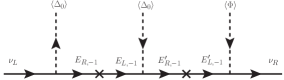
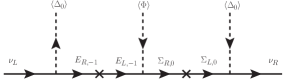
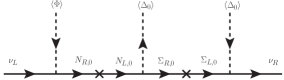
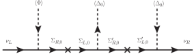
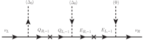
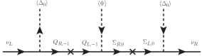
Figure 17: Diagrams showing the $T_{5}$ topology of the operator $\bar{L}\bar{\Phi}\bar{\Delta}_{0}\Delta_{0}\nu_{R}$.

,    ,    ,    ,    ,   

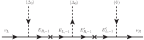
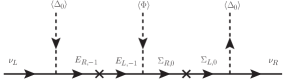
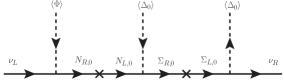
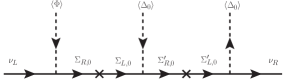
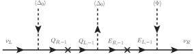
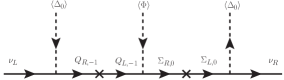
Figure 18: Diagrams showing the $T_{5}$ topology of the operator $\bar{L}\bar{\Phi}\bar{\Delta}_{0}\Delta_{0}\nu_{R}$.

Notice that the contractions in Fig. 17 and the ones in Fig. 18 differ just in the exchange of $\Delta\leftrightarrow\bar{\Delta}$. While these diagrams involve messengers having similar transformations under the Standard Model gauge group, they differ from each other in how they transform under the symmetry group used to forbid lower dimensional operators. This also implies that the messenger pairs $E_{-1}$ and $E^{\prime}_{-1}$ as well as $\Sigma_{0}$ and $\Sigma^{\prime}_{0}$ must be different from each other. Keeping this in mind we have counted them as different UV-complete models.

For the operator $\bar{L}\otimes\bar{\Phi}\otimes\bar{\Delta}_{-2}\otimes\Delta_{-2}\otimes\nu_{R}$ the first and second contractions of (27) are forbidden due to messenger fields not having any neutral component. For the same reason, the third contractions of (25) and (27) are forbidden for the operator $\bar{L}\otimes\Phi\otimes\Delta_{0}\otimes\Delta_{-2}\otimes\nu_{R}$. For the case of the operator $\bar{L}\otimes\bar{\Phi}\otimes\Delta_{0}\otimes\Delta_{0}\otimes\nu_{R}$ all the contractions in (27) and (28) are indistinguishable from those in (25) and (26) and hence should not be counted as separate contractions.

VII Discussion and Summary

As a follow-up to our recent paper in Ref. CentellesChulia:2018gwr , here we have classified and analysed the various ways to generate Dirac neutrino mass through the use of dimension-6 operators. The UV-completion of such scenarios will require new messenger fields carrying $SU(2)_{L}\otimes U(1)_{Y}$ charges that may be probed at colliders, since the scale involved may be phenomenologically accessible. By using only the Standard Model Higgs doublet in the external legs one has a unique operator, Eq. (2). We have shown, however, that the presence of new scalars implies the existence of many possible field contractions. We have described in detail the simplest ones of these, involving $SU(2)_{L}$ singlets, doublets and triplets. In order to ensure the Dirac nature of neutrinos, as well as the seesaw origin of their mass (in our case, at the dimension-6 level) extra symmetries are needed. They can be realized in several ways, a simple example being lepton quarticity. Such symmetries can also be used to provide the stability of dark matter. In fact one should emphasize the generality of this connection, already explained in Ref. CentellesChulia:2018gwr in the context of the dimension-5 Dirac seesaw scenario.

- (1) S. Centelles Chulia, R. Srivastava and J. W. F. Valle, Seesaw roadmap to neutrino mass and dark matter (2018), arXiv:1802.05722 [hep-ph].
- (2) J. Schechter and J. W. F. Valle, Neutrinoless Double beta Decay in SU(2) x U(1) Theories, Phys.Rev. D25 2951.
- (3) A. Gando et al. (KamLAND-Zen Collaboration), Search for Majorana Neutrinos near the Inverted Mass Hierarchy Region with KamLAND-Zen, Phys. Rev. Lett. 117 (2016) 8 082503, Addendum: Phys. Rev. Lett.117, 109903 (2016), arXiv:1605.02889 [hep-ex].
- (4) M. Agostini et al. (GERDA Collaboration), Improved Limit on Neutrinoless Double-beta decay of 76Ge from GERDA Phase II, Phys. Rev. Lett. 120 (2018) 132503.
- (5) C. E. Aalseth et al. (MAJORANA Collaboration), Search for Zero-Neutrino Double Beta Decay in 76Ge with the Majorana Demonstrator 120 (2018) 132502.
- (6) C. Alduino et al. (CUORE Collaboration), First Results from CUORE: A Search for Lepton Number Violation via Decay of 130Te, Phys. Rev. Lett. 120 (2018) 132501.
- (7) J. Albert et al. (EXO-200 Collaboration), Search for Neutrinoless Double-Beta Decay with the Upgraded EXO-200 Detector, Phys. Rev. Lett. 120 (2018) 072701.
- (8) R. Arnold et al. (NEMO-3), Measurement of the Decay Half-Life and Search for the Decay of 116Cd with the NEMO-3 Detector, Phys. Rev. D95 (2017) 1 012007, arXiv:1610.03226 [hep-ex].
- (9) J. Schechter and J. W. F. Valle, Neutrino Masses in SU(2) x U(1) Theories, Phys. Rev. D22 (1980) 2227.
- (10) P. Chen et al., Warped flavor symmetry predictions for neutrino physics, JHEP 01 (2016) 007, arXiv:1509.06683 [hep-ph].
- (11) A. Addazi, J. W. F. Valle and C. A. Vaquera-Araujo, String completion of an electroweak model, Phys. Lett. B759 (2016) 471–478, arXiv:1604.02117 [hep-ph].
- (12) S. Centelles Chuliá et al., Dirac Neutrinos and Dark Matter Stability from Lepton Quarticity, Phys. Lett. B767 209–213, arXiv:1606.04543 [hep-ph].
- (13) S. Centelles Chuliá et al., CP violation from flavor symmetry in a lepton quarticity dark matter model, Phys. Lett. B761 431–436, arXiv:1606.06904 [hep-ph].
- (14) S. Centelles Chulia, R. Srivastava and J. W. F. Valle, Generalized Bottom-Tau unification, neutrino oscillations and dark matter: predictions from a lepton quarticity flavor approach, Phys. Lett. B773 (2017) 26–33, arXiv:1706.00210 [hep-ph].
- (15) J. Heeck and W. Rodejohann, Neutrinoless Quadruple Beta Decay, EPL 103 (2013) 3 32001, arXiv:1306.0580 [hep-ph].
- (16) G. Abbas, S. Gupta, G. Rajasekaran and R. Srivastava, High Scale Mixing Unification for Dirac Neutrinos, Phys. Rev. D91 (2015) 11 111301, arXiv:1312.7384 [hep-ph].
- (17) E. Ma and R. Srivastava, Dirac or inverse seesaw neutrino masses with gauge symmetry and flavor symmetry, Phys. Lett. B741 (2015) 217–222, arXiv:1411.5042 [hep-ph].
- (18) H. Okada, Two loop Induced Dirac Neutrino Model and Dark Matters with Global Symmetry arXiv:1404.0280 [hep-ph].
- (19) E. Ma and R. Srivastava, Dirac or Inverse Seesaw Neutrino Masses from Gauged Symmetry, Adv. Ser. Direct. High Energy Phys. 25 (2015) 165–174.
- (20) E. Ma and R. Srivastava, Dirac or inverse seesaw neutrino masses from gauged symmetry, Mod. Phys. Lett. A30 (2015) 26 1530020, arXiv:1504.00111 [hep-ph].
- (21) E. Ma, N. Pollard, R. Srivastava and M. Zakeri, Gauge Model with Residual Symmetry, Phys. Lett. B750 (2015) 135–138, arXiv:1507.03943 [hep-ph].
- (22) J. W. F. Valle and C. A. Vaquera-Araujo, Dynamical seesaw mechanism for Dirac neutrinos, Phys. Lett. B755 (2016) 363–366, arXiv:1601.05237 [hep-ph].
- (23) C. Bonilla and J. W. F. Valle, Naturally light neutrinos in model, Phys. Lett. B762 (2016) 162–165, arXiv:1605.08362 [hep-ph].
- (24) C. Bonilla, E. Ma, E. Peinado and J. W. F. Valle, Two-loop Dirac neutrino mass and WIMP dark matter, Phys. Lett. B762 (2016) 214–218, arXiv:1607.03931 [hep-ph].
- (25) M. Reig, J. W. F. Valle and C. A. Vaquera-Araujo, Realistic model with a type II Dirac neutrino seesaw mechanism, Phys. Rev. D94 (2016) 3 033012, arXiv:1606.08499 [hep-ph].
- (26) E. Ma and O. Popov, Pathways to Naturally Small Dirac Neutrino Masses, Phys. Lett. B764 142–144, arXiv:1609.02538 [hep-ph].
- (27) W. Wang and Z.-L. Han, Naturally Small Dirac Neutrino Mass with Intermediate Multiplet Fields arXiv:1611.03240 [hep-ph].
- (28) D. Borah and A. Dasgupta, Common Origin of Neutrino Mass, Dark Matter and Dirac Leptogenesis, JCAP 1612 12 034, arXiv:1608.03872 [hep-ph].
- (29) G. Abbas, M. Z. Abyaneh and R. Srivastava, Precise predictions for Dirac neutrino mixing, Phys. Rev. D95 (2017) 7 075005, arXiv:1609.03886 [hep-ph].
- (30) C.-Y. Yao and G.-J. Ding, Systematic Study of One-Loop Dirac Neutrino Masses and Viable Dark Matter Candidates, Phys. Rev. D96 (2017) 9 095004, arXiv:1707.09786 [hep-ph].
- (31) E. Ma and U. Sarkar, Radiative Left-Right Dirac Neutrino Mass, Phys. Lett. B776 (2018) 54–57, arXiv:1707.07698 [hep-ph].
- (32) D. Borah and A. Dasgupta, Naturally Light Dirac Neutrino in Left-Right Symmetric Model arXiv:1702.02877 [hep-ph].
- (33) W. Wang, R. Wang, Z.-L. Han and J.-Z. Han, The Scotogenic Models for Dirac Neutrino Masses arXiv:1705.00414 [hep-ph].
- (34) C. Bonilla et al., Flavour-symmetric type-II Dirac neutrino seesaw mechanism (2017), arXiv:1710.06498 [hep-ph].
- (35) M. Hirsch, R. Srivastava and J. W. F. Valle, Can one ever prove that neutrinos are Dirac particles? (2017), arXiv:1711.06181 [hep-ph].
- (36) R. Srivastava et al., Testing a lepton quarticity flavor theory of neutrino oscillations with the DUNE experiment (2017), arXiv:1711.10318 [hep-ph].
- (37) D. Borah and B. Karmakar, Flavour Model for Dirac Neutrinos: Type I and Inverse Seesaw (2017), arXiv:1712.06407 [hep-ph].
- (38) C.-Y. Yao and G.-J. Ding, Systematic Analysis of Dirac Neutrino Masses at Dimension Five (2018), arXiv:1802.05231 [hep-ph].
- (39) S. Centelles Chuliá, Dirac neutrinos, dark matter stability and flavour predictions from Lepton Quarticity, in 7th International Pontecorvo Neutrino Physics School Prague, Czech Republic, August 20-September 1, 2017 (2017) arXiv:1711.10719 [hep-ph], URL http://inspirehep.net/record/1639438/files/arXiv:1711.10719.pdf.
- (40) R. M. Fonseca, M. Hirsch and R. Srivastava, processes: Proton decay and LHC (2018), arXiv:1802.04814 [hep-ph].
- (41) J. C. Helo, M. Hirsch and T. Ota, Proton decay and light sterile neutrinos (2018), arXiv:1803.00035 [hep-ph].
- (42) M. Reig, D. Restrepo, J. W. F. Valle and O. Zapata, Bound-state dark matter and Dirac neutrino mass (2018), arXiv:1803.08528 [hep-ph].
- (43) R. N. Mohapatra and J. W. F. Valle, Neutrino mass and baryon-number nonconservation in superstring models, Phys. Rev. D34 1642.
- (44) M. Gonzalez-Garcia and J. Valle, Fast Decaying Neutrinos and Observable Flavor Violation in a New Class of Majoron Models, Phys.Lett. B216 360.
- (45) D. Binosi and L. Theussl, JaxoDraw: A Graphical user interface for drawing Feynman diagrams, Comput. Phys. Commun. 161 (2004) 76–86, arXiv:hep-ph/0309015 [hep-ph].