A Comparative Study of Full-Duplex Relaying Schemes for Low Latency Applications

Abstract

[Abstract]Various sectors are likely to carry a set of emerging applications while targeting a reliable communication with low latency transmission. To address this issue, upon a spectrally-efficient transmission, this paper investigates the performance of a one full-dulpex (FD) relay system, and considers for that purpose, two basic relaying schemes, namely the symbol-by-symbol transmission, i.e., amplify-and-forward (AF) and the block-by-block transmission, i.e., selective decode-and-forward (SDF). The conducted analysis presents an exhaustive comparison, covering both schemes, over two different transmission modes, i.e., the non combining mode where the best link, direct or relay link is decoded and the signals combining mode, where direct and relay links are combined at the receiver side. While targeting latency purpose as a necessity, simulations show a refined results of performed comparisons, and reveal that AF relaying scheme is more adapted to combining mode, whereas the SDF relaying scheme is more suitable for non combining mode.

1 Introduction

An immense amount of data is created every day from different sensors and peripherals, namely, GPS embedded in vehicles, attached to objects or worn by people, sensors monitoring the environment, real time video streams, radars on roads, social network feeds, etc. Such type of data belongs to real time’s domain, where schedulability is one of the main characteristics of this domain, which means its propensity to respect the expected time constraints. In fact a real time system implies a system ability to ensure that investigated processing produces consistent results, i.e., functionally correct, at the right time. Therefore, to ensure the radio communication for such applications, a low latency as well as extreme reliability are required. In this context, the use of cooperation concept provides spatial and temporal diversity, and constitutes a good alternative to support advanced communications with increased channel capacity ^{1, 2}.

However, in regards to the end-to-end latency, this requirement has a significant impact on the system quality and the fluidity of communications, and it is influenced by different features upon the transmission, we mention in particular, the propagation delay as well as the relay delay processing. In fact, depending on the environment and on the application, we can get rid of some supplementary sources of delay, as example, for industrial environments such factories, the distance between two automated robots is not considerable. Hence, the delay propagation can be neglected, and the only generated delay in this case, is that related to the relay processing, which depends mainly on the used relaying technique.

In general, there are various ways of relay processing in cooperative networks, among which we distinct mainly two familiar relaying schemes: amplify-and-forward (AF) and decode-and-forward (DF) ³. In AF scheme, the relay simply amplifies the received signal and forwards it towards the destination. Thus, in term of the relay processing delay, the AF scheme, does not include a prominent latency ⁴. However, this relaying scheme suffers from noise amplification. In the DF scheme, the relay first decodes the signal received from the source, re-encodes and re-transmits it to the destination. This approach suffers from error propagation when the relay transmits an erroneously decoded data block. Selective DF (SDF), where the relay only transmits when it can reliably decode the data packet, has been introduced as an efficient method to reduce error propagation ⁵.

In the perspective of a low latency, full-duplex (FD) relaying mode allows fast device-to-device discovery, and hence, contributes on the delay reduction. Furthermore, as the capacity improvement is promoted by the spectral efficiency improvement, the adoption of the FD communication at the relay is more advantageous. Even if full-duplex relaying mode FD generates loop interference from relay input to relay output, it still practical to use on cooperative relaying system due to its spectral efficiency ^{6, 7, 8}. The FD relay requires the duplication of radio frequency circuits to transmits and receives simultaneously in the same time slot and in the same frequency band. It has been shown that the FD mode still feasible even with the presence of a significant loop interference ⁶, especially with recent advances noted in antenna technology and signal processing techniques. In ⁹, a novel technique for self-interference cancellation using antenna cancellation is depicted for FD transmissions. In the same context, through passive suppression and active self-interference cancellation mechanisms, an experiment study was proposed in ¹⁰. Hence, these practical growth incites authors to adopt FD communications in their research, thus, get rid of spectral inefficiency caused by half-duplex relaying mode.

1. Contributions

Most of previous available works in the literature have investigated the performance analysis of cooperative networks based SDF and AF relaying schemes, with the regard to different purposes ^{11, 12, 13, 14, 15, 16, 17}. In ¹¹, considering the FD-AF relaying over Nakagami-$m$ fading channel, authors cover the performances based on outage probability and ergodic capacity. The authors in ^{12, 13, 14, 15, 16, 17} adopt a FD cooperative scheme with the direct link between the source and the destination nodes is non-negligible. Still, in ^{12, 13, 14}, to capture the joint benefit of relaying and direct links, at the destination side, authors have assumed a silence period at the source that is equal to the processing delay at the relay. The work in ¹⁷, investigates over a Rayleigh fading channel, the optimal mode selection upon a FD-AF system and study therefore, the individual impact of the residual self-interference (RSI) and the direct link on the outage performance. However, none of the cited works have evaluated the relevance in term of latency impact in the context of latency sensitive applications.

In this paper, we address this issue by conducting a refined comparison between AF and SDF relaying schemes. Note that each of them adopts a different block transmission scheme. The pertinence of the direct link effect is also investigated, through the assumption of two different transmission modes, i.e., the non combining mode and the signals combining mode. For that purpose, over the so called Nakagami-$m$ block-fading channel, we elaborate first the studied transmission schemes communication model, then we derive their outage probability expressions. Theoretical results are represented with Monte-carlo simulations and show, on the basis of a low needed latency, the relevance of each relaying technique, according to the operating transmission mode.

The rest of the paper is organized as follows: section 2 presents the studied system model. The outage probabilities are derived in section 3. In section 4, numerical performance results are shown and discussed. The paper is concluded in section 5.

Notations

• $x$, $\mathbf{x}$, and $\mathbf{X}$ denote, respectively, a scalar quantity, a column vector, and a matrix.

• $\mathcal{G}\left(m,\alpha\right)$ represents Gamma distribution with shape parameter $m$ and rate parameter $\alpha$.

• $\mathcal{CN}\left(\mu,\sigma\right)$ represents a circularly symmetric complex Gaussian distribution with mean $\mu$ and variance $\sigma$.

• $\delta_{m,n}$ is the Kronecker symbol, i.e., $\delta_{m,n}=1$ for $m=n$ and $\delta_{m,n}=0$ for $m\neq n$.

• $\left(.\right)^{\star}$,$\left(.\right)^{\top}$, and $\left(.\right)^{\mathrm{H}}$ are conjugate, the transpose, and the Hermitian transpose, respectively.

• $\mathbb{C}$ is set of complex number.

• For $\mathbf{x}\in\mathbb{C}^{N\times 1}$, $\mathbf{x}_{f}$ denotes the discrete Fourier transform (DFT) of $\mathbf{x}$, i.e. $\mathbf{x}_{f}=\mathbf{U}_{N}\mathbf{x}$, with $\mathbf{U}_{N}$ is a unitary $N\times N$ matrix whose $\left(m,n\right)$th element is $\left(\mathbf{U}_{N}\right)_{m,n}=\frac{1}{\sqrt{N}}e^{-j(2\pi mn/N)}$, $j=\sqrt{-1}$.

• $\left|.\right|$ denotes the absolute value.

• $\mathbb{{E}}\left\{.\right\}$ is used to denote the statistical expectation.

• $\mathrm{Pr}\left(X\right)$ is the probability of occurrence of the event $X$.

2 System Model

This section presents a signal model for one relay cooperative system, where a FD relay $(\mathrm{R})$, assists the communication between two end users, representing respectively, the source $(\mathrm{S})$ and the destination $(\mathrm{D})$. In this paper, we assume the direct link between the source and the destination nodes is non-negligible. Since relay operates in FD mode, we take into account the RSI generated from relay’s input to relay’s output. We consider both, the non-regenerative and regenerative relaying schemes, namely, amplify-and-forward and selective decode-and-forward. Hereafter, we introduce first, the adopted channel model for analysis, then, investigate the system model, covering both, the AF and the SDF schemes, over two different transmission modes, i.e., the non-combining mode where the best link, direct or relay link is decoded and the combining mode, where direct and relay links are combined at the receiver side.

2.1 channel model

The source-destination $\mathrm{S\rightarrow D}$, source-relay $\mathrm{S\rightarrow R}$, the relay self-interference, and relay-destination $\mathrm{R\rightarrow D}$ channels, are represented by $h_{\mathrm{\mathrm{ab}}},$ with $\mathrm{ab}\epsilon\left\{\mathrm{SD},\,\mathrm{SR},\,\mathrm{RR},\,\mathrm{RD}\right\}$. In this paper, we assume that $h_{\mathrm{Z}}$, $Z\epsilon\left\{\mathrm{SR},\,\mathrm{RD,}\,\mathrm{SD}\right\}$, are modeled by independent Nakagami-$m$ fading with shape parameter $m_{\mathrm{Z}}$ and average power $\mathbb{{E}}\left\{\left|h_{\mathrm{Z}}\right|^{2}\right\}=\sigma_{Z}^{2}$ . Thus, the squared magnitudes $\left|h_{Z}\right|^{2}$ are Gamma distributed with shape parameter $m_{\mathrm{Z}}$ and rate parameter $\alpha_{\mathrm{Z}}=\frac{m_{Z}}{\sigma_{\mathrm{Z}}^{2}}$, i.e., $\left|h_{\mathrm{Z}}\right|^{2}\sim\mathcal{G}\left(m_{\mathrm{Z}},\alpha_{\mathrm{Z}}\right)$ . The probability density function (PDF) and the cumulative density function (CDF) of a Gamma random variable $X\sim\mathcal{G}\left(m,\alpha\right)$ are, respectively, given by

$$f_{X}(x)=\frac{\alpha^{m}}{\Gamma(m)}\times x^{m-1}\times e^{-\alpha x},$$ (1)

and

$$F_{X}\left(x\right)=\frac{\gamma(m,\alpha x)}{\Gamma(m)},\qquad x\geq 0,$$ (2)

where $\Gamma(.)$ denotes the Gamma function and $\gamma(.\,,\,.)$ denotes the lower incomplete Gamma function.

2.2 Signal model

At channel use i, the source node broadcasts its signal $x_{s}(i)$ to both the relay and the destination. Accordingly, the received signal at the relay and the destination, during channel use i, can be expressed, respectively, as:

$$y_{\mathrm{R}}(i)=\sqrt{P_{\mathrm{s}}}h_{\mathrm{SR}}x_{\mathrm{s}}(i)+h_{\mathrm{RR}}x_{\mathrm{R}}(i)+n_{\mathrm{R}}(i),$$ (3)

$$y_{\mathrm{D}}(i)=\underset{\mathrm{Direct\,signal}}{\underbrace{a\mathrm{{}_{SD}}x_{\mathrm{s}}(i)}}+\underset{\mathrm{Relayed\,signal}}{\underbrace{a_{\mathrm{RD}}x_{\mathrm{s}}(i-\tau)}}+\eta_{\mathrm{D}}(i),$$ (4)

with $a\mathrm{{}_{SD}=\sqrt{P_{\mathrm{s}}}h_{\mathrm{SD}}}$, $\mathbb{{E}}\left[x_{\mathrm{s}}(i)x_{\mathrm{s}}^{\star}(i^{\prime})\right]=\delta_{i,i^{\prime}}$, $P_{\mathrm{s}}$ denotes the transmit power at the source, $\tau$ is the processing delay at the relay, and $h_{\mathrm{RR}}x_{\mathrm{R}}(i)$ is the RSI after undergoing any cancellation techniques and practical isolation at the relay ^{7, 18}, and is assumed to be equivalent to a zero mean complex Gaussian random variable $\sim\mathcal{CN}(0,\sigma_{\mathrm{RR}}^{2})$. $n_{\mathrm{R}}\sim\mathcal{CN}(0,N_{r})$ denotes, a zero-mean complex additive white Gaussian noise at the relay. Both $a_{\mathrm{RD}}$ and $\eta_{\mathrm{D}}\sim\mathcal{CN}(0,\zeta_{D}^{2})$ depend on the relaying scheme.

• Amplify-and-forward: With AF scheme, the relay acts as a repeater which simply amplify the received signal and forwards it to the destination. Thereby,

$$\begin{cases}a_{RD}=\beta\sqrt{P_{\mathrm{s}}}h_{\mathrm{RD}}h_{\mathrm{SR}}\\ \eta_{D}(i)=\underset{\mathrm{RSI}}{\underbrace{\beta h_{\mathrm{RD}}h_{\mathrm{RR}}x_{\mathrm{R}}(i-\tau_{\mathrm{AF}})}}+\underset{\mathrm{Noise}}{\underbrace{\beta h_{\mathrm{RD}}n_{\mathrm{R}}(i-\tau_{\mathrm{AF}})+n_{\mathrm{D}}(i)}}\end{cases}$$ (5)

where $\beta=\sqrt{\frac{P_{\mathrm{R}}}{P_{\mathrm{s}}|h_{\mathrm{SR}}|^{2}+P_{\mathrm{R}}\sigma_{\mathrm{RR}}^{2}+N_{r}}}$ is the amplification constant factor chosen to satisfy the total power constraint at the relay ¹¹, $P_{\mathrm{R}}$ denotes the transmit power at the relay, $\tau_{AF}$ is the AF relay processing delay, and $n_{\mathrm{D}}\sim\mathcal{CN}(0,N_{\mathrm{D}})$ denotes a zero-mean complex additive white Gaussian noise at the destination.

• Selective decode-and-forward: In SDF scheme, the relay retransmits the received signal only when the $\mathrm{S}\rightarrow\mathrm{R}$ link is not in outage. For this scheme, $\eta_{D}(i)=n_{\mathrm{D}}(i)$ and

$$a_{\mathrm{RD}}=\begin{cases}\sqrt{P_{\mathrm{R}}}h_{\mathrm{\mathrm{R}D}}&\textrm{if\,$\mathrm{S}\rightarrow\mathrm{R\,}$link\,not\,in\,outage}\\ 0&\textrm{otherwise}\end{cases}$$ (6)

From equation (4), we see that the destination node receives the source transmitted signal $x_{\mathrm{s}}$ at different time instances due to the processing delay $\tau$ at the relay. In this work, we consider two transmission modes: Non combining (NC) mode where the receiver is synchronized with the strongest link, direct or relay link, and Signals combining (SC) mode where both direct and relay links are combined at the receiver side.

2.2.1 Non Combining (NC) mode

In this mode, the destination will try to decode the strongest link while, the second one will be considered as interference. Therefore, the system capacity of the NC mode for AF and SDF is expressed respectively, as:

$$C_{NC}^{AF}=\mathrm{log_{2}\left(1\text{+}\gamma_{AF}\right)}$$ (7)

$$C_{NC}^{SDF}=\mathrm{log_{2}\left(1\text{+}\gamma_{SDF}\right),}$$ (8)

with $\mathrm{\gamma_{AF}}=\frac{|a\mathrm{{}_{XD}}|^{2}}{|a_{\mathrm{\overline{X}D}}|^{2}+\beta^{2}|h_{\mathrm{RD}}|^{2}(P_{\mathrm{R}}\sigma_{\mathrm{RR}}^{2}+N_{\mathrm{r}})+N_{D}}$ and $\mathrm{\gamma_{SDF}}=\frac{P_{\mathrm{R}}|h_{\mathrm{XD}}|^{2}}{P_{\mathrm{\mathrm{s}}}|h_{\mathrm{\overline{X}D}}|^{2}+N_{D}}$, are respectively, the AF and SDF signal-to-interference and noise ratio (SINR), where $\mathrm{X}\rightarrow\mathrm{D}$ is the best link and $\mathrm{\overline{X}}\rightarrow\mathrm{D}$ is the worst link considered as interference.

2.2.2 Signals Combining (SC) mode

In SC mode both relay and direct signals are combined at the destination side. Therefore, in order to alleviate the inter-symbol interference (ISI) caused by the delayed signal, equalization is performed at the destination. For that purpose, we propose a cyclic-prefix (CP) transmission at the source side in order to perform frequency-domain equalization (FDE) at the destination node. Depending on the processing protocol at the relay, AF or SDF, the destination performs signal-based FDE or block-based FDE. In the following, we assume all channel gains remain constant during $N+\tau_{\mathrm{CP}}$ channel uses, where $\tau_{\mathrm{CP}}$ is the CP length ($\tau_{\mathrm{CP}}\geq\mathit{\tau}$).

At the destination side, after the CP removal, the received signal, at channel use $i$, can be expressed as,

$$y_{\mathrm{D}}(i)=\underset{\mathrm{Direct\,+\,Relayed\,signal}}{\underbrace{\sqrt{P_{\mathrm{s}}}h_{\mathrm{SD}}x_{\mathrm{s}}(i)+a_{\textrm{RD}}x_{\mathrm{s}}\left[(i-\tau)\,\mathrm{mod}\,N\right]}}+\eta_{\mathrm{D}}(i),$$ (9)

Equation (9) can be written in vector form to jointly take into account the $N+\tau$ received signal as:

$$\mathbf{y}_{D}=\boldsymbol{{\mathcal{H}}}\mathbf{x}_{\mathrm{s}}+\boldsymbol{\mathbf{\eta_{D}}},$$ (10)

where $\mathbf{y}_{D}=\left[y_{D}\left(0\right),...,y_{D}\left(N-1\right)\right]^{\top}\in\mathbb{C}^{N\times 1}$, $\mathbf{x}_{\mathrm{s}}=\left[x_{\mathrm{s}}\left(0\right),...,x_{\mathrm{s}}\left(N-1\right)\right]^{\top}\in\mathbb{C}^{N\times 1}$, $\mathbf{\boldsymbol{\eta}_{D}}=\left[\eta_{\mathrm{D}}\left(0\right),...,\eta_{\mathrm{D}}\left(N-1\right)\right]^{\top}\in\mathbb{C}^{N\times 1}$ , and $\boldsymbol{{\mathcal{H}}}\in\mathbb{C}^{N\times N}$ is a circulant matrix whose first column matrix is $\left[a\mathrm{{}_{SD}},\boldsymbol{{0}}_{1\times\tau-2},a_{\textrm{RD}},\boldsymbol{{0}}_{1\times N-\tau}\right]^{\top}$. Note that the circulant matrix $\boldsymbol{{\mathcal{H}}}$ , can be decomposed as, $\boldsymbol{{\mathcal{H}}}=\mathbf{U}_{N}^{H}\boldsymbol{{\Lambda}}\mathbf{U}_{N}$. With $\boldsymbol{{\Lambda}}$ is a diagonal matrix whose $\left(i,i\right)$-th element is $\lambda_{i}=a\mathrm{{}_{SD}}+a_{\textrm{RD}}e^{-j\left(2\pi i\frac{\tau}{N}\right)}.$ Therefore, the signal $\mathbf{y}_{\mathrm{D}}$ can be represented in the frequency domain as,

$$\mathbf{y}_{\mathrm{D}_{f}}=\boldsymbol{{\Lambda}}\mathbf{x}_{\mathrm{s}_{f}}+\mathbf{n}_{f}.$$ (11)

At the destination side, the system capacity is given by,

$$C_{\mathrm{SC}}=\left(\frac{N}{N+\tau}I(\mathbf{x}_{\mathrm{s}_{f}},\mathbf{y}_{\mathrm{D}_{f}})\right),$$ (12)

where the factor $\frac{N}{N+\tau}$ means that the transmission of $N$ useful bits occupies $N+\tau$ channel uses and $I$ represents the overall system average mutual information, and is given by, $I(\mathbf{x}_{\mathrm{s}_{f}},\mathbf{y}_{\mathrm{D}_{f}})=\frac{1}{N}{\displaystyle\sum_{i=0}^{N-1}}\mathrm{log_{2}}(1+\gamma_{i})$, where $\gamma_{i}=\frac{\lambda_{i}\lambda_{i}^{H}}{\zeta_{D}^{2}}=\rho+2\left|\mu\right|cos\left(2\pi i\frac{\tau}{N}+\theta\right)$, with $\rho=\frac{|a_{\mathrm{\mathrm{S}D}}|^{2}+|a_{\mathrm{RD}}|^{2}}{\zeta_{D}^{2}}$, $\mu=\frac{a_{\mathrm{\mathrm{S}D}}a_{\mathrm{RD}}}{\zeta_{D}^{2}}$, and $\theta=angle\left(h\mathrm{{}_{SD}},h_{\mathrm{RD}}^{*}\right)$.

The system mutual information $I(\mathbf{x}_{\mathrm{s}_{f}},\mathbf{y}_{\mathrm{D}_{f}})$ can be manipulated as below,

$$I(\mathbf{x}_{\mathrm{s}_{f}},\mathbf{y}_{\mathrm{D}_{f}}) =\frac{1}{N}\sum_{i=0}^{N-1}\mathrm{log_{2}}(1+\gamma_{i})$$

$$=\frac{1}{N}\sum_{i=0}^{N-1}\mathrm{log_{2}}\left[(1+\rho)\left(1+\frac{2\left|\mu\right|cos\left(2\pi i\frac{\tau}{N}+\theta\right)}{1+\rho}\right)\right]$$ (13)

$$=\mathrm{log_{2}}(1+\rho)+\frac{1}{N}\sum_{i=0}^{N-1}\mathrm{log_{2}}\left(1+\frac{2\left|\mu\right|cos\left(2\pi i\frac{\tau}{N}+\theta\right)}{1+\rho}\right).$$

According to the arithmetic-geometric mean inequality, $\rho\geq 2\left|\mu\right|$, we have $1+\rho>2\left|\mu\right|cos\left(2\pi i\frac{\tau}{N}+\theta\right).$ Thus, by using the first order Taylor expansion, we have $\mathrm{ln}\left(1+\frac{2\left|\mu\right|cos\left(2\pi i\frac{\tau}{N}+\theta\right)}{1+\rho}\right)\thickapprox\frac{2\left|\mu\right|cos\left(2\pi i\frac{\tau}{N}+\theta\right)}{1+\rho}.$ Noting that ${\displaystyle\sum_{i=0}^{N-1}}cos\left(2\pi i\frac{\tau}{N}+\theta\right)=0$, the mutual information, in (13), can be approximated as,

$$I(\mathbf{x}_{\mathrm{s}_{f}},\mathbf{y}_{\mathrm{D}_{f}}) \thickapprox\mathrm{log_{2}}(1+\rho)$$ (14)

• Amplify-and-Forward: AF is classified as memoryless scheme in which the relay processes the received signal in a symbol-by-symbol manner. Therefore, the processing delay $\tau_{AF}$ is in term of channel uses and thus, the equalization, at the destination side, is a signal-based equalization.

• Selective Decode and Forward: Unlike AF, SDF is a memory scheme where the entire received block need to be decoded, before deciding to retransmit or not the re-encoded block through $\mathrm{R}\rightarrow\mathrm{D}$ link. This results in a block-based processing delay $\tau_{\mathrm{SDF}}$. Thereby, as depicted in Fig.1, to deal with inter-block interferences, the communication takes place assuming one superblock transmission of $L$ blocks, each gathering $N$ symbols and the SDF CP prefix is constructed using D blocks of $N$, i.e., $\tau_{\mathrm{SDF}}=D\times N$.

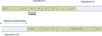
Figure 1: SDF Block transmission scheme

3 Outage Probability

In this section, we present the outage analysis of different schemes investigated in section 2. The system outage occurs when the received SINR at the destination side is below a target SNR threshold, whether for SC mode, where both relay and direct signals are combined at the destination side, or NC mode, where the destination will try to decode the strongest link while, the second one will be considered as interference. Note that, in this work, the packet re-transmission is not considered.
Hereafter, we derive first for each mode, i.e. NC and SC, the overall full-duplex outage probability of the AF scheme as well as that of the SDF ¹³. For the purpose of investigating the analysis, let’s first introduce the instantaneous SINRs for each link.

The received SINR of the $\mathrm{S}\rightarrow\mathrm{D}$, the $\mathrm{S}\rightarrow\mathrm{R}$ and the $\mathrm{R}\rightarrow\mathrm{D}$ links are denoted, respectively, as,

$$\gamma_{\mathsf{S\mathrm{D}}} =\frac{P_{\mathrm{s}}|h_{\mathrm{SD}}|^{2}}{N_{\mathrm{D}}},\,\gamma_{\mathrm{SR}}=\frac{P_{\mathrm{s}}|h_{\mathrm{\mathrm{SR}}}|^{2}}{P_{\mathrm{R}}\sigma_{\mathrm{RR}}^{2}+N_{\mathrm{r}}},\,\gamma_{\mathrm{RD}}=\frac{P_{\mathrm{R}}|h_{\mathrm{RD}}|^{2}}{N_{\mathrm{D}}}.$$ (15)

Note that $\gamma_{\mathrm{SR}}$, $\gamma_{\mathrm{SD}}$ and $\gamma_{\mathrm{RD}}$ are the result of a Gamma random variable scaled by a constant. Therefore, $\gamma_{\mathrm{SR}}$, $\gamma_{\mathrm{SD}}$ and $\gamma_{\mathrm{RD}}$ are Gamma distributed with shape parameter $m_{\mathrm{Z}}$ and rate parameter $\tilde{\alpha}_{\mathrm{Z}}$, where $\tilde{\alpha}_{\mathrm{SD}}=\frac{N_{\mathrm{D}}}{P_{\mathrm{S}}}\alpha_{\mathrm{SD}}$, $\tilde{\alpha}_{\mathrm{{SR}}}=\frac{P_{\mathrm{R}}\sigma_{\mathrm{RR}}^{2}+N_{\mathrm{r}}}{P_{\mathrm{S}}}\alpha_{\mathrm{SR}}$ and $\tilde{\alpha}_{\mathrm{RD}}=\frac{N_{r}}{P_{\mathrm{R}}}\alpha_{\mathrm{RD}}$.

Herein, the outage probability is denoted $P_{\mathrm{out}}$ and expressed as:

$$P_{\mathrm{out}}= \mathrm{Pr}(\gamma<\eta)$$ (16)

$$= F_{\gamma}\left(\eta\right),$$

where $\eta=2^{R}-1$, with $R$ is the bit rate per channel use, and $F_{\gamma}\left(.\right)$ is the CDF of $\gamma$.

3.1 Non combining mode

Herein, for the rest of NC mode analysis, we consider $\eta_{AF}=\eta_{SDF}=\eta=2^{R}-1$.

• Amplify-and-forward

For AF relaying scheme, using (15), we extract the corresponding end-to-end SINR as,

$$\mathrm{\gamma_{AF}}=\begin{cases}\frac{\gamma_{\mathrm{SR}}\frac{\gamma_{\mathrm{RD}}}{\gamma_{\mathrm{SD}+1}}}{\gamma_{\mathrm{SR}}+\frac{\gamma_{\mathrm{RD}}}{\gamma_{\mathrm{SD}+1}}+1}.&if\,\gamma_{\mathrm{RD}}>\gamma_{\mathrm{SD}}\\ \frac{\gamma_{\mathrm{SD}}}{\gamma_{\mathrm{RD}+1}}&otherwise\end{cases}$$ (17)

Herein, for the case where the $\mathrm{R}\rightarrow\mathrm{D}$ link is stronger than the $\mathrm{S\rightarrow D}$, after some manipulations, the equation (16), tends to an integral form which doesn’t generate a closed form expression, and can be evaluated numerically using matlab software. Otherwise, using ¹³ Eq 12, the outage probability can be derived as,

$$F_{\mathrm{\gamma_{AF}}}(\eta)=\frac{\gamma(m_{\mathrm{SD}},\tilde{\alpha}_{\mathrm{SD}}\eta)}{\Gamma(m_{\mathrm{SD}})}+B\sum_{k=0}^{m_{\mathrm{RD}}-1}c^{-d}\tilde{\alpha}_{\mathrm{\mathrm{RD}}}^{k}W_{a,b}[c],$$ (18)

where $W_{a,b}[c]$ denotes, the Whittaker function, $a=\frac{m_{\mathrm{SD}}-k-1}{2}$, $b=\frac{-m_{\mathrm{SD}}-k}{2}$, $c=\tilde{\alpha}_{\mathrm{SD}}\eta+\tilde{\alpha}_{\mathrm{\mathrm{RD}}}$, $d=\frac{m_{\mathrm{SD}}+k+1}{2}$, and $B=\frac{e^{-\left(\frac{1}{2}\left(\tilde{\alpha}_{\mathrm{SD}}\eta-\tilde{\alpha}_{\mathrm{\mathrm{RD}}}\right)\right)}}{\Gamma(m_{\mathrm{SD}})}\left(\tilde{\alpha}_{\mathrm{SD}}\eta\right)^{m_{\mathrm{SD}}}$.

• Selective Decode and Forward

The SDF relay system outage probability, is generally, defined as:

$$\begin{aligned} \mathcal{P}_{\mathrm{out}}&=P_{\mathrm{out}}^{\mathrm{S\rightarrow D}}P_{\mathrm{out}}^{\mathrm{S\rightarrow R}}+\mathit{P_{\mathrm{out}}^{\mathcal{\mathrm{X}}\mathrm{D}}}\left(1-P_{\mathrm{out}}^{\mathrm{S\rightarrow R}}\right)\end{aligned},$$ (19)

where $P_{\mathrm{out}}^{\mathrm{S\rightarrow D}}$ and $P_{\mathrm{out}}^{\mathrm{S\rightarrow R}}$ denote respectively, the outage probability of $\mathrm{S\rightarrow D}$ link and $\mathrm{S\rightarrow R}$ link, and can be expressed as in ¹³,

$$P_{\mathrm{out}}^{\mathrm{S\rightarrow D}}= \frac{\gamma(m_{\mathrm{SD}},\tilde{\alpha}_{\mathrm{SD}}\eta)}{\Gamma(m_{\mathrm{SD}})}$$ (20)

$$P_{\mathrm{out}}^{\mathrm{S\rightarrow R}}= \frac{\gamma(m_{\mathrm{SR}},\tilde{\alpha}_{\mathrm{SR}}\eta)}{\Gamma(m_{\mathrm{SR}})}$$ (21)

$\mathit{P_{\mathrm{out}}^{\mathcal{\mathrm{X}}\mathrm{D}}}$ denotes the outage probability of the best link $\mathrm{X\rightarrow D}$, i.e., $\mathrm{R\rightarrow D}$ or $\mathrm{S\rightarrow D}$, when the relay correctly decodes the received signal, and it can be derived as follows,

$$\mathit{P_{\mathrm{out}}^{\mathrm{X}\mathrm{D}}}= \mathrm{Pr}\left(\gamma_{\mathrm{SDF}}<\eta\right)$$

$$= F_{\gamma_{\mathrm{SDF}}}(\eta)$$ (22)

and it is given by the following expression ¹³ Eq. 12:

$$F_{\gamma_{\mathrm{SDF}}}(\eta)=\frac{\gamma(m_{\mathrm{XD}},\tilde{\alpha}_{\mathrm{XD}}\eta)}{\Gamma(m_{\mathrm{XD}})}+B\sum_{k=0}^{m_{\mathrm{\overline{X}D}}-1}c^{-d}\tilde{\alpha}_{\mathrm{\mathrm{\overline{X}D}}}^{k}W_{a,b}[c],$$ (23)

where $W_{a,b}[c]$ denotes, the Whittaker function, $a=\frac{m_{\mathrm{XD}}-k-1}{2}$, $b=\frac{-m_{\mathrm{XD}}-k}{2}$, $c=\tilde{\alpha}_{\mathrm{XD}}\eta+\tilde{\alpha}_{\mathrm{\mathrm{\overline{X}D}}}$, $d=\frac{m_{\mathrm{XD}}+k+1}{2}$, and $B=\frac{e^{-\left(\frac{1}{2}\left(\tilde{\alpha}_{\mathrm{XD}}\eta-\tilde{\alpha}_{\mathrm{\mathrm{\overline{X}D}}}\right)\right)}}{\Gamma(m_{\mathrm{XD}})}\left(\tilde{\alpha}_{\mathrm{XD}}\eta\right)^{m_{\mathrm{XD}}}$.

Finally, by substituting (20), (21), and (23) into (19), we get the closed form expression of NC SDF outage probability.

3.2 Signals Combining mode

• Amplify-and-forward

The outage probability of FD AF combining system is derived as follows:

$$P_{\mathrm{out}} = \mathrm{Pr}\left(\frac{N}{N+\tau_{AF}}\mathrm{log_{2}}(1+\rho)<r\right)$$ (24)

$$= F_{\rho}\left(\eta_{AF}\right),$$

where $\eta_{AF}=2^{R\left(\frac{N+\tau_{AF}}{N}\right)}-1$. By substituting (15) into $\rho$, we get,

$$\rho= \frac{\gamma_{\mathrm{SR}}\gamma_{\mathrm{RD}}+\gamma_{\mathrm{SD}}\gamma_{\mathrm{SR}}+\gamma_{\mathrm{SD}}}{1+\gamma_{\mathrm{SR}}+\gamma_{\mathrm{RD}}}.$$ (25)

Thus, the CDF of $\rho$ can be derived as,

$$F_{\rho}\left(x\right) =\mathrm{Pr}(\rho<x)=\mathrm{Pr}\left(\gamma_{\mathrm{SD}}\leq\underset{\mathrm{\Delta}}{\underbrace{\frac{(1+\gamma_{\mathrm{SR}}+\gamma_{\mathrm{RD}})x-\gamma_{\mathrm{SR}}\gamma_{\mathrm{RD}}}{1+\gamma_{\mathrm{SR}}}}}\right)$$

$$=\iint_{\Delta\geq 0}\frac{\gamma(m_{\mathrm{SD}},\tilde{\alpha}_{\mathrm{SD}}\Delta)}{\Gamma(m_{\mathrm{SD}})}\times f_{\gamma_{\mathrm{SR}}}(y)\times f_{\gamma_{\mathrm{RD}}}(z)dydz.$$ (26)

where $\gamma(l,x)$ presents the lower incomplete Gamma function ¹⁹.

Hereafter, to solve this double integral, we need to decompose the integration into two steps. Therefore, in order to proceed, let’s denote $g(\gamma_{\mathrm{SR}},z)=\frac{\gamma(m_{\mathrm{SD}},\tilde{\alpha}_{\mathrm{SD}}\Delta)}{\Gamma(m_{\mathrm{SD}})}\times f_{\gamma_{\mathrm{RD}}}(z)$. First, while treating $\gamma_{\mathrm{SR}}$ as constant, we have to integrate $g(\gamma_{\mathrm{SR}},z)$ with respect to the limits $\begin{cases}z_{1}=\left(\frac{1+\gamma_{\mathrm{SR}}}{\gamma_{\mathrm{SR}}-\eta_{AF}}\right)\eta_{AF}\,\textrm{and}\,z_{2}=\infty,&\textrm{if}\,\gamma_{\mathrm{SR}}\leq\eta_{AF}\\ z_{1}=0\,\textrm{and}\,z_{2}=\left(\frac{1+\gamma_{\mathrm{SR}}}{\gamma_{\mathrm{SR}}-\eta_{AF}}\right)\eta_{AF},&\textrm{if}\,\gamma_{\mathrm{SR}}>\eta_{AF}\end{cases}$. Using the serie form, i.e. $\gamma(l,x)=(l-1)!\left[1-e^{-x}{\displaystyle\sum_{a=0}^{l-1}}\frac{x^{a}}{a!}\right]$ ¹⁹ 8.352.6 and the polynomial expansion, i.e. $(x+1)^{a}={\displaystyle\sum_{b=0}^{a}}\frac{a!}{b!(a-b)!}x^{b}$, we get therefore, the first integral resolution, i.e., $G\left(\eta_{AF}\right)$ as represented in (27).

$$G\left(\eta_{AF}\right)=\begin{cases}1-{\displaystyle\sum_{a=0}^{m_{\mathrm{SD}}-1}}{\displaystyle\sum_{b=0}^{a}}\frac{\left(\frac{\eta_{AF}-\gamma_{\mathrm{SR}}}{\eta_{AF}\left(1+\gamma_{\mathrm{SR}}\right)}\right)^{b}\times\left(\tilde{\alpha}_{\mathrm{SD}}\eta_{AF}\right)^{a}}{b!(a-b)!}\times\frac{\Gamma\left(m_{\mathrm{RD}}+b\right)}{\left(\tilde{\alpha}_{\mathrm{RD}}+\left(\frac{\eta_{AF}-\gamma_{\mathrm{SR}}}{1+\gamma_{\mathrm{SR}}}\right)\tilde{\alpha}_{\mathrm{SD}}\right)^{(m_{\mathrm{RD}}+b)}}\times\frac{e^{(-\tilde{\alpha}_{\mathrm{SD}}\eta_{AF})}\times\tilde{\alpha}_{\mathrm{RD}}^{m_{\mathrm{RD}}}}{\Gamma(m_{\mathrm{RD}})},&\gamma_{\mathrm{SR}}\leq\eta_{AF}\\ \frac{\gamma\left(m_{RD},\tilde{\alpha}_{\mathrm{RD}}\left(\frac{1+\gamma_{\mathrm{SR}}}{\gamma_{\mathrm{SR}}-\eta_{AF}}\right)\eta_{AF}\right)}{\Gamma(m_{\mathrm{RD}})}-{\displaystyle\sum_{a=0}^{m_{\mathrm{SD}}-1}}{\displaystyle\sum_{b=0}^{a}}\frac{\left(\frac{\eta_{AF}-\gamma_{\mathrm{SR}}}{\eta_{AF}\left(1+\gamma_{\mathrm{SR}}\right)}\right)^{b}\times\left(\tilde{\alpha}_{\mathrm{SD}}\eta_{AF}\right)^{a}}{b!(a-b)!}\times\frac{\gamma\left(m_{\mathrm{RD}}+b,\tilde{\alpha}_{\mathrm{RD}}\left(\frac{1+\gamma_{\mathrm{SR}}}{\gamma_{\mathrm{SR}}-\eta_{AF}}\right)\eta_{AF}-\tilde{\alpha}_{\mathrm{SD}}\eta_{AF}\right)}{\left(\tilde{\alpha}_{\mathrm{RD}}+\left(\frac{\eta_{AF}-\gamma_{\mathrm{SR}}}{1+\gamma_{\mathrm{SR}}}\right)\tilde{\alpha}_{\mathrm{SD}}\right)^{(m_{\mathrm{RD}}+b)}}\\ \times\frac{e^{\left(-\tilde{\alpha}_{\mathrm{SD}}\eta_{AF}\right)}\times\tilde{\alpha}_{\mathrm{RD}}^{m_{\mathrm{RD}}}}{\Gamma(m_{\mathrm{RD}})},&\gamma_{\mathrm{SR}}>\eta_{AF}\end{cases}$$ (27)

Now, the resulting expression, i.e., $G\left(\eta_{AF}\right)$ is integrated accordingly with respect to bounds, as represented in (28).

$$F_{\rho}\left(\eta_{AF}\right)= \intop_{0}^{\eta_{AF}}\left(1-\sum_{a=0}^{m_{\mathrm{SD}}-1}\sum_{b=0}^{a}\frac{\left(\frac{\eta_{AF}-y}{\eta_{AF}\left(1+y\right)}\right)^{b}\times\left(\tilde{\alpha}_{\mathrm{SD}}\eta_{AF}\right)^{a}}{b!(a-b)!}\times\frac{\Gamma\left(m_{\mathrm{RD}}+b\right)}{\left(\tilde{\alpha}_{\mathrm{RD}}+\left(\frac{\eta_{AF}-y}{1+y}\right)\tilde{\alpha}_{\mathrm{SD}}\right)^{(m_{\mathrm{RD}}+b)}}\times\frac{e^{(-\tilde{\alpha}_{\mathrm{SD}}\eta_{AF})}\times\tilde{\alpha}_{\mathrm{RD}}^{m_{\mathrm{RD}}}}{\Gamma(m_{\mathrm{RD}})}\right)\times f_{\gamma_{\mathrm{SR}}}(y)\,dy+$$ (28)

$$\intop_{\eta_{AF}}^{\infty}\Biggl{(}\frac{\gamma\left(m_{RD},\tilde{\alpha}_{\mathrm{RD}}\left(\frac{1+y}{y-\eta_{AF}}\right)\eta_{AF}\right)}{\Gamma(m_{\mathrm{RD}})}-\sum_{a=0}^{m_{\mathrm{SD}}-1}\sum_{b=0}^{a}\frac{\left(\frac{\eta_{AF}-y}{\eta_{AF}\left(1+y\right)}\right)^{b}\times\left(\tilde{\alpha}_{\mathrm{SD}}\eta_{AF}\right)^{a}}{b!(a-b)!}\times$$

$$\frac{\gamma\left(m_{\mathrm{RD}}+b,\tilde{\alpha}_{\mathrm{RD}}\left(\frac{1+y}{y-\eta_{AF}}\right)\eta_{AF}-\tilde{\alpha}_{\mathrm{SD}}\eta_{AF}\right)}{\left(\tilde{\alpha}_{\mathrm{RD}}+\left(\frac{\eta_{AF}-y}{1+y}\right)\tilde{\alpha}_{\mathrm{SD}}\right)^{(m_{\mathrm{RD}}+b)}}\times\frac{e^{\left(-\tilde{\alpha}_{\mathrm{SD}}\eta\right)}\times\tilde{\alpha}_{\mathrm{RD}}^{m_{\mathrm{RD}}}}{\Gamma(m_{\mathrm{RD}})}\Biggr{)}\times f_{\gamma_{\mathrm{SR}}}(y)\,dy,$$

Finally, (28) is manipulated, to get thus, the AF outage expression, i.e., $F_{\rho}\left(\eta_{AF}\right)$ as depicted in (29).

$$F_{\rho}\left(\eta_{AF}\right)= 1-\frac{\tilde{\alpha}_{\mathrm{SR}}^{m_{\mathrm{SR}}}}{\Gamma(m_{\mathrm{SR}})\Gamma(m_{\mathrm{RD}})}\intop_{\eta_{AF}}^{\infty}y^{m_{\mathrm{SR}}-1}e^{-\tilde{\alpha}_{\mathrm{SR}}y}\times\Gamma\left(m_{\mathrm{RD}},\tilde{\alpha}_{\mathrm{RD}}\left(\frac{1+y}{y-\eta_{AF}}\right)\eta_{AF}\right)dy-$$ (29)

$$\frac{e^{(-\tilde{\alpha}_{\mathrm{SD}}\eta_{AF})}\times\tilde{\alpha}_{\mathrm{RD}}^{m_{\mathrm{RD}}}\times\tilde{\alpha}_{\mathrm{SR}}^{m_{\mathrm{SR}}}}{\Gamma(m_{\mathrm{RD}})\Gamma(m_{\mathrm{SR}})}\sum_{a=0}^{m_{\mathrm{SD}}-1}\sum_{b=0}^{a}\frac{\left(\tilde{\alpha}_{\mathrm{SD}}\eta_{AF}\right)^{a}}{b!(a-b)!}\times$$

$$\Biggl{(}\intop_{0}^{\infty}\frac{\Gamma\left(m_{\mathrm{RD}}+b\right)\left(\frac{\eta_{AF}-y}{\eta_{AF}\left(1+y\right)}\right)^{b}y^{m_{\mathrm{SR}}-1}e^{-\tilde{\alpha}_{\mathrm{SR}}y}}{\left(\tilde{\alpha}_{\mathrm{RD}}+\left(\frac{\eta_{AF}-y}{1+y}\right)\tilde{\alpha}_{\mathrm{SD}}\right)^{(m_{\mathrm{RD}}+b)}}dy-\intop_{\eta_{AF}}^{\infty}\frac{\left(\frac{\eta_{AF}-y}{\eta_{AF}\left(1+y\right)}\right)^{b}y^{m_{SR}-1}e^{-\tilde{\alpha}_{\mathrm{SR}}y}}{\left(\tilde{\alpha}_{\mathrm{RD}}+\left(\frac{\eta_{AF}-y}{1+y}\right)\tilde{\alpha}_{\mathrm{SD}}\right)^{(m_{\mathrm{RD}}+b)}}\times$$

$$\Gamma\left(m_{\mathrm{RD}}+b,\tilde{\alpha}_{\mathrm{RD}}\left(\frac{1+y}{y-\eta_{AF}}\right)\eta_{AF}-\tilde{\alpha}_{\mathrm{SD}}\eta_{AF}\right)dy\Biggr{)}$$

The integrals generally, do not generate a closed form expression, thus, it can be evaluated numerically using matlab software.

• Selective Decode and Forward

In the following, we briefly introduce the FD SDF relay system outage probability. In SC mode, if the relay correctly decodes the received packet, and decides to re-transmit the re-encoded block through the $\mathrm{R}\rightarrow\mathrm{D}$ link, both relay and direct links are combined at the destination side. This mode’s outage probability is generally, denoted as the same form as (19). However, the threshold will be redefined accordingly as, $\eta_{\mathrm{SDF}}=2^{R\left(\frac{NL+\tau_{SDF}}{NL}\right)}-1$, and $\mathit{P_{\mathrm{out}}^{\mathrm{XD}}}$ in $(\ref{eq:sdfout})$ will be denoted, $\mathit{P_{\mathrm{out}}^{\mathrm{S}\mathcal{\mathrm{R}}\mathrm{D}}}$, which represents the outage probability of the combined signal, i.e., direct and relayed signals, at the destination side, and it can be derived as follows,

$$\mathit{P_{\mathrm{out}}^{\mathrm{S}\mathcal{\mathrm{R}}\mathrm{D}}}=\mathrm{Pr}\left(\frac{1}{NL+\tau_{SDF}}\sum_{i=0}^{NL-1}\log_{2}(1+\gamma_{i})<r\right).$$ (30)

Hence, by referring to ^{12, 13}, the end-to-end SINR, can be approximated to $\gamma_{i}\approx\gamma_{\mathrm{SD}}+\gamma_{\mathrm{RD}}$ . Thus, using (14) and (15), the expression of $\mathit{P_{\mathrm{out}}^{\mathrm{S}\mathcal{\mathrm{R}}\mathrm{D}}}$ is approximated and given by,

$$\mathit{P_{\mathrm{out}}^{\mathrm{S}\mathcal{\mathrm{R}}\mathrm{D}}}\approx \mathrm{Pr}\left(\frac{NL}{NL+\tau_{SDF}}\log_{2}\left(1+\gamma_{\mathrm{SD}}+\gamma_{\mathrm{RD}}\right)<r\right).$$

Therefore, $P_{\mathrm{out}}^{\mathrm{S}\mathcal{\mathrm{R}}\mathrm{D}}$ can be derived as:

$$\mathit{P_{\mathrm{out}}^{\mathrm{S}\mathcal{\mathrm{R}}\mathrm{D}}}= \mathrm{Pr}\left(\gamma_{\mathrm{SD}}+\gamma_{\mathrm{RD}}<\eta_{\mathrm{SDF}}\right)$$

$$= \intop_{0}^{\eta_{\mathrm{SDF}}}\mathrm{Pr}\left(\gamma_{\mathrm{SD}}<\eta_{\mathrm{SDF}}-y\right)\times f_{\gamma_{\mathrm{RD}}}(y)\textrm{d}y,$$ (31)

Hereafter, while developing the integral form, we got the expression of $P_{out}^{\mathrm{S}\mathcal{\mathrm{R}}\mathrm{D}}$, as given in ¹³,

$$\mathit{P_{out}^{\mathrm{S}\mathcal{\mathrm{R}}\mathrm{D}}}= \frac{\gamma(m_{\mathrm{RD}},\tilde{\alpha}_{\mathrm{RD}}\eta_{\mathrm{SDF}})}{\Gamma(m_{\mathrm{RD}})}-\sum_{k=0}^{m_{\mathrm{SD}}-1}\left(\tilde{\alpha}_{\mathrm{SD}}\eta_{SDF}\right)^{k}\times\frac{\left(\tilde{\alpha}_{\mathrm{RD}}\eta_{SDF}\right)^{m_{\mathrm{RD}}}\times e^{-\left(\tilde{\alpha}_{\mathrm{RD}}\eta_{SDF}\right)}}{\Gamma(m_{\mathrm{RD}}+k+1)}$$

$$\times {}_{1}F_{1}\left(k+1;m_{\mathrm{RD}}+k+1;\tilde{\alpha}_{\mathrm{RD}}-\tilde{\alpha}_{\mathrm{SD}}\right).$$ (32)

where ${}_{1}F_{1}\left(k+1;m_{\mathrm{RD}}+k+1;\tilde{\alpha}_{\mathrm{RD}}-\tilde{\alpha}_{\mathrm{SD}}\right)$ denotes the Kummer’s confluent hypergeometric function.

Finally, by substituting (20), (21) and (32) into (19), we get the closed form expression of SDF outage probability.

4 Numerical Results

In this section, the theoretical findings derived in section 3, are numerically verified and confirmed using Monte-carlo simulations. The variation of outage probability for various transmission schemes investigated in section 2, is represented. Moreover, for an exhaustive comparison, simulations include the direct transmission mode with no relay cooperation. To assess SC-SDF performances in term of super block length, we consider two cases: 1) the case where the super-block length is very large compared with the relay processing delay, $N\times L\gg\tau_{SDF}$ , 2) and the case of short super-block where $L=3$. In this section, the first case is denoted SC-SDF while the second case is denoted SC-SDF3. For all simulations, we consider a packet length of $N=20$ symbols, and a relay processing delay of $\tau_{AF}=1$ symbol for symbol-by-symbol transmissions and $\tau_{SDF}=500\,\textrm{$\mu$s}$ for block-by-block transmissions. $P_{\mathrm{S}}=P_{\mathrm{R}}=5\,\textrm{dB}$ and $m_{\textrm{SD}}=m_{\textrm{SR}}=m_{\textrm{RD}}=2$.

First, we compare the studied relaying schemes performances in term of the spectral efficiency level. For that purpose, in Fig.3 and Fig.3, we plot the outage probability versus the transmission bit rate R. First, we notice that the simulation results confirm the accuracy of the analytical expressions, obtained in section 3. In both figures, we note that, for transmissions that support very long super-block, i.e., $\frac{NL}{NL+\tau_{SDF}}\rightarrow 1$, the SC-SDF offers the best performances. However, for transmissions with low latency requirements less than $1$ ms, the super-block length must be less than $L=3$. Thus, using SC-SDF is not anymore the obvious choice. Thereafter, in term of the low latency purpose, we see that, in Fig. 3, when the direct link gain is very low compared to the first and second hop gains, the low processing delay scheme, SC-AF scheme, offers the best performance. However, as the direct link gain increases, we start to notice that SC-SDF3 becomes more desirable for low transmission rate, while the SC-AF still the best choice for high transmission rate. This is mainly due to the SDF rate penalty of $\frac{NL}{NL+\tau_{SDF}}$ that impacts banefully the spectral efficiency, whenever the super block size decreases.

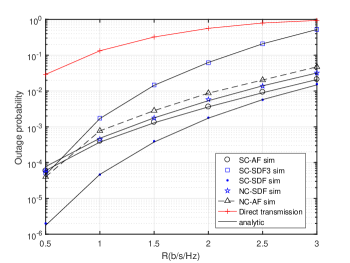
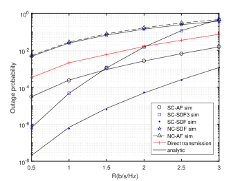
Figure 2: Outage probability versus $R$ , for $\sigma_{\mathrm{SR}}^{2}=\sigma_{\mathrm{RD}}^{2}=20\,\mathrm{dB}$, $\sigma_{\mathrm{SD}}^{2}=0\,\mathrm{dB}$ and $\sigma_{\mathrm{RR}}^{2}=0\mathrm{\,dB}$.

Figure 3: Outage probability versus $R$ , for $\sigma_{\mathrm{SR}}^{2}=\sigma_{\mathrm{RD}}^{2}=20\,\mathrm{dB}$, $\sigma_{\mathrm{SD}}^{2}=10\,\mathrm{dB}$ and $\sigma_{\mathrm{RR}}^{2}=0\mathrm{\,dB}$.

Hereafter, to point out the impact of the RSI level on performances, Fig. 5 and Fig. 5 illustrate the outage probabilities as function of $\sigma_{RR}^{2}$. In one hand, we see clearly that SC-SDF still provides the best performance. However, this scheme can not be practically adopted for low latency transmissions. In the other hand, we notice that there are three transmission schemes that outperform each other depending on the RSI level at the relay and can be practically adopted for low latency transmissions: SC-AF, NC-SDF, and direct transmission. In fact, SC-AF seems to be the most suitable scheme for low latency transmissions with low RSI at the relay, i.e., $\sigma_{RR}^{2}\leq 5$ dB. However, for moderate and high RSI, i.e., $\sigma_{RR}^{2}>5\,\textrm{dB}$, we can either use NC-SDF if the direct link is not strong enough (Fig. 5) or just switch-off the relay if the direct link gain is as good as the relay link (Fig. 5). In fact, in Fig. 5, we see that the direct transmission clearly outperforms NC-SDF scheme. This is due to the fact that, in NC mode, the destination will try to decode the strongest received signal while the remaining signal will be considered as interference. Accordingly, at low RSI, where the relay can correctly decode and forward the re-encoded block, the destination will receive a useful signal as strong as the interfering signal, which dramatically deteriorates the system performances. As the RSI gain increases, i.e., $\sigma_{RR}^{2}>5\,\textrm{dB}$, the relay fails to correctly decode the received packet. Therefore, the only received signal at destination is the direct link signal. That is clearly seen in Fig. 5 where the NC-SDF curve improves, as the $\sigma_{RR}^{2}$ increases, to be similar to the direct transmission curve.

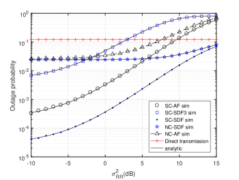
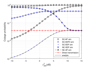
Figure 4: Outage probability versus $\sigma_{\mathrm{RR}}^{2}$ , for $R=2$bps/Hz, $\sigma_{\mathrm{SR}}^{2}=\sigma_{\mathrm{RD}}^{2}=20\,\mathrm{dB}$ and $\sigma_{\mathrm{SD}}^{2}=5\,\mathrm{dB}$

Figure 5: Outage probability versus $\sigma_{\mathrm{RR}}^{2}$ , for $R=2$bps/Hz, $\sigma_{\mathrm{SR}}^{2}=\sigma_{\mathrm{RD}}^{2}=10\,\mathrm{dB}$ and $\sigma_{\mathrm{SD}}^{2}=8\,\mathrm{dB}$ .

Now, we consider the scenario where the $\mathrm{S}\rightarrow\mathrm{R}$ link is much better than the $\mathrm{S}\rightarrow\mathrm{D}$ link, i.e., $\sigma_{\mathrm{SR}}^{2}=\sigma_{\mathrm{SD}}^{2}+10\,\mathrm{dB}$. Fig.7 and Fig.7 plot the outage probability versus a range of $\mathrm{S}\rightarrow\mathrm{R}$ link gains. We see clearly that, for moderate $\mathrm{R}\rightarrow\mathrm{D}$ link quality, i.e., $\sigma_{\mathrm{RD}}^{2}=5\,\mathrm{dB}$, SC-AF scheme offers better outage performance than all other studied schemes. On the other hand, as the $\mathrm{R}\rightarrow\mathrm{D}$ link variance increases, i.e., $\sigma_{\mathrm{RD}}^{2}=20\mathrm{\,dB}$, we notice that the performance of NC modes are enhanced for low $\mathrm{S}\rightarrow\mathrm{D}$ link gain, i.e., $\sigma_{\mathrm{SD}}^{2}<5\,\mathrm{dB}$, where the direct link harmful impact becomes negligible. Indeed, a performance gap between the NC-SDF and the SC-SDF3 can be specifically noticed, when the $\mathrm{S}\rightarrow\mathrm{D}$ link gain becomes lower, at above, $\sigma_{\mathrm{SD}}^{2}<6\,\mathrm{dB}$. Therefore, in this case, if considering the SDF protocol, it is rather better to choose the NC mode than the SC. While with strong $\mathrm{S}\rightarrow\mathrm{D}$ link, the SC modes are more suitable for transmission scenarios, mainly due to the additional spatial diversity. Moreover, the SC-AF presents higher performances for higher $\mathrm{S}\rightarrow\mathrm{R}$ link gains, which is obvious as a result.

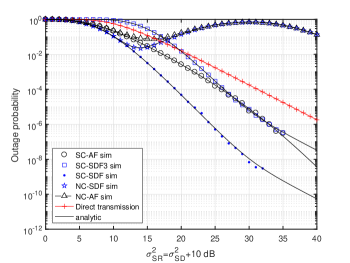
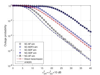
Figure 6: Outage probability versus $\sigma_{\mathrm{SR}}^{2}$ , for $R=2$bps/Hz, $\sigma_{\mathrm{RD}}^{2}=20\,\mathrm{dB}$ and $\sigma_{\mathrm{RR}}^{2}=0\mathrm{\,dB}$.

Figure 7: Outage probability versus $\sigma_{\mathrm{SR}}^{2}$, for $R=2$bps/Hz, $\sigma_{\mathrm{RD}}^{2}=5\,\mathrm{dB}$ and $\sigma_{\mathrm{RR}}^{2}=0\mathrm{\,dB}$.

5 Conclusion

Two basic cooperative relaying schemes, i.e. AF and SDF, were studied over a Nakagami-m fading channel, where one FD relay assisted the communication between a source node and a destination node. For an exhaustive comparison, we adopted both relaying protocols over two different transmission mode, i.e., the non-combining mode and the signals combining mode. Simulations results, proved that the SDF block-based transmission scheme is no longer practical to adopt for FD SC mode, where direct and relay links are combined at the receiver side, especially, with the more latency induced due to the complexity of encoding and decoding algorithms. Still the AF scheme represents better choice in term of outage performance and latency. On the other hand, SDF relaying scheme is more suitable for non combining transmission mode.

References

• 1 J. Han, J. Baek, S. Jeon and J. Seo, “Cooperative networks with amplify-and-forward multiple-full-duplex relays”, IEEE Transactions on Wireless Communications, Vol. 13, no. 4, pp. 2137 - 2149, April 2014.
• 2 A. F. M. Shahen Shah and Md. Shariful Islam, “A survey on cooperative communication in wireless networks”, I.J. Intelligent Systems and Applications, pp. 66-78, June 2014.
• 3 J. N. Laneman, D. Tse, and G. W. Wornell, “Cooperative diversity in wireless networks: Efficient protocols and outage behavior”, IEEE Trans. Inform. Theory, vol. 50, no. 12, pp. 3062-3080, Dec. 2004.
• 4 N. Nikaein and S. Krea, “Latency for Real-Time Machine-to-Machine Communication in LTE-Based System Architecture”, in Proc. IEEE European Wireless, Vienna, Austria, April 2011.
• 5 F. Atay Onat, H. Yanikomeroglu, and S. Periyalwar, “Relay-assisted spatial multiplexing in wireless fixed relay networks”, IEEE GLOBECOM, San Francisco, USA, Nov.- Dec. 2006.
• 6 T. Riihonen, S. Werner, R. Wichman, and E. Zacarias, "On the feasibility of full-duplex relaying in the presence of loop interference", in Proc. IEEE SPAWC, Perugia, Italy, June 2009.
• 7 T. Riihonen, S. Werner, and R. Wichman, “Optimized gain control for single-frequency relaying with loop interference,” IEEE Transactions on Wireless Communications, vol. 8, no. 6, pp. 2801-2806, June 2009.
• 8 T. Kwon, S. Lim, S. Choi, and D. Hong, “Optimal duplex mode for DF relay in terms of the outage probability,” IEEE Transactions on Vehicular Technology, vol. 57, no. 7, pp. 3628 –3634, Sept. 2010.
• 9 J. I. Choi, M. Jain, K. Srinivasan, P. Levis, and S. Katti, “Achieving single channel, full duplex wireless communication,” in Proc. ACM MobiCom, Chicago, Illinois, USA, September 2010.
• 10 M. Duarte, C. Dick, and A. Sabharwal, “Experiment-driven characterization of full-duplex wireless systems,” IEEE Transactions on Wireless Communications, vol. 11, no. 12, pp. 4296-4307, May 2012.
• 11 Z. Shi, S. Ma, F. Hou, and K. W. Tam, “Analysis on full-duplex amplify-and-forward relay networks under nakagami fading channels,” in Proc. IEEE GLOBECOM, pp. 1-6, Dec. 2015.
• 12 M. G. Khafagy, A. Ismail, M. S. Alouini, and S. Aissa, “On the outage performance of full-duplex selective decode-and-forward relaying,” IEEE Communications Letters, vol. 17, no. 6, pp. 1180-1183, Apr. 2013.
• 13 M. G. Khafagy, A. Ismail, M. S. Alouini, and S. Aissa, “Efficient cooperative protocols for full-duplex relaying over nakagami-fading channels,” IEEE Transactions on Wireless Communications, vol. 14, no .6, pp. 3456-3470, Feb. 2015.
• 14 Q. Wang, Y. Dong, X. Xu, and X. Tao, “Outage probability of full-duplex AF relaying with processing delay and residual self-Interference,” IEEE Communications Letters, vol. 19, no. 5, pp. 783-786, Mar. 2015.
• 15 D. M. Osorio, E. B. Olivo, H. Alves, J. C. S. Santos Filho, and M. Latva-aho, “Exploiting the direct link in full-duplex amplify-and-forward relaying networks”, IEEE Signal Processing Letters, vol. 22, no. 10, pp. 1766-1770, Oct 2015.
• 16 Y. Wang, K. Xu, Y. Li, Y. Xu, X. Shen, and F. Wang, "Outage performance of full-duplex selective decode-and-forward relaying over Nakagami-m fading channels", in Proc. IEEE WCSP, Nanjing, China, Oct 2015.
• 17 T. M. Kim and A. Paulraj, “Outage probability of amplify-and-forward cooperation with full duplex relay”, in Proc. IEEE WCNC, Shanghai, China, April 2012.
• 18 M. Jain, J. Choi, T. Kim, D. Bharadia, S. Seth, K. Srinivasan, P. Levis, S. Katti, and P. Sinha, “Practical, real-time, full duplex wireless”, in Proc. ACM MobiCom, Las Vegas, Nevada, USA, September 2011.
• 19 I. Gradshteyn, I. Ryzhik : “Table of integrals, series and products”, $7^{th}$ edition. London: Academic Press, 2007.
• 20 Study on Latency Reduction Techniques for LTE (Release 14), document TR 36.881, 3rd Generation Partnership Project (3GPP), 2016. [Online]. Available: http://www.3gpp.org/dynareport/36881.htm
• 21 A. A. Zaidi , R. Baldemair, H. Tullberg, H. Bjorkegren, L. Sundstrom, J. Medbo, and I. Da Silva, “Waveform and numerology to support 5G services and requirements”, IEEE Communications Magazine, vol. 54, no. 11, pp. 90-98, 2016.